Article

Assessing Hydrus-2D Model to Investigate the Effects of Different On-Farm Irrigation Strategies on Potato Crop under Subsurface Drip Irrigation

1
Department of Plant Biotechnology, Higher Institute of Biotechnology of Beja, Avenue Habib Bourguiba, B.P: 382, Béja 9000, Tunisia
2
Department of Agriculture, Food and Environment (DAFE), University of Pisa, Via del Borghetto 80, 56124 Pisa, Italy
3
Unit of Sousse, Olive Institute, Ibn Khaldoun 14, Sousse 4061, Tunisia
4
Department of Rural Engineering, High Agronomic Institute of Chott Mériem, Université de Sousse, BP 47, Chott Mériem Sousse 4042, Tunisia
5
Department Agriculture, Food and Forest Sciences, Università degli Studi di Palermo, Viale delle Scienze 12, Ed.4, 90128 Palermo, Italy
*
Author to whom correspondence should be addressed.
Water 2019, 11(3), 540; https://doi.org/10.3390/w11030540
Submission received: 18 February 2019 / Revised: 28 February 2019 / Accepted: 11 March 2019 / Published: 15 March 2019
(This article belongs to the Section Water Use and Scarcity)

Abstract

:
The objective of this paper was to assess the performance of Hydrus-2D model to simulate the effects of different on-farm irrigation strategies applied on potato crop. The ability of the model to simulate the stress coefficient (Ks), obtained as the ratio between actual and maximum transpiration, and to define the productive function of potato crop under the semi-arid conditions of central Tunisia were also evaluated. Experiments were carried out on potato crop under full (FI) and deficit irrigation (DI) and two different water qualities supplied by means of a subsurface drip irrigation system. Results evidenced that the model, despite some discrepancies locally observed, can fairly accurately predict soil water contents and electrical conductivity around buried emitters. Furthermore, under water and salt stress conditions, “measured” Ks, based on crop water stress index (CWSI) obtained on thermal images, resulted in a good correlation with the corresponding estimated by the model (R2 = 0.8). The database collected during the three growth seasons also allowed the definition of the crop productive function represented by a linear relationship between the relative yield loss and Ks. This function represents a useful guidelines for the sustainable use of irrigation water in countries characterized by a semi-arid climate and a limited availability of water for irrigation.

1. Introduction

In semi-arid regions like central Tunisia, the scarcity of water and the quality of available resources oblige the adoption of water management strategies aimed to increase water use efficiency. In Tunisia, irrigated surfaces have increased more than six times in the last half century and, with a percentage of 8% of the potential cultivable lands, provide about 35% of total agricultural production [1,2]. Moreover, due to the chronic scarcity of good quality water, farmers are quite often obliged to use marginal waters, such as wastewaters or saline waters, whose application could cause salt accumulation in the soil and the reductions of crop yield [3,4,5]. Compared to some arboreal crops or cereals, horticultural crops are more water demanding. With more than 50 varieties, potato represents the second main crop in Tunisia, with a harvested area in 2017 of 25,590 ha and a total production of 420,000 tons [6]. In order to increase irrigation water use efficiency, even for potato crop, on the one hand it is necessary to design correctly irrigation units accounting for energy, cost, and uniformity [7], even considering the role of local losses on distribution uniformity [8,9] and, from the other, to identify irrigation strategies aimed to optimize crop water use [10,11]. The correct choice of the sowing time can also affect the irrigation regime with positive implications on water use efficiency. Bowen [12] evidenced that under Mediterranean climate, drought, and heat stress are the main abiotic stresses occurring simultaneously during dry periods, and therefore fresh tuber yield is greater during winter than in summer. Compared to other methods, drip irrigation is considered one of the most efficient [13,14,15]. However, the most effective way to increase water use efficiency (WUE) is the precise control of irrigation [16]. Recently, different water saving strategies have been proposed to reduce crop water requirements with limited or no effects on crop yield. Deficit irrigation is an optimization strategy in which water restriction is limited to the drought-tolerant crop growth stages. Application of this strategy has been extensively documented for potato crop [17,18,19,20,21], even if several researchers evidenced the difficulty to manage crop water stress and to verify the effects on tuber yield [22,23,24]. To this aim, several researches have been focusing on the relationships between crop transpiration fluxes or amounts of irrigation water supply and crop yield. Stewart et al. [25] evidenced that seasonal evapotranspiration and crop yield are linearly related, with a slope that is sensitive to climatic factors, but that could be affected by the crop variety.
In the late seventies, the Food and Agriculture Organization of the United Nations [FAO] proposed the adoption of the “water production function” as a practical procedure to quantify the effects of evapotranspiration reductions on yield losses [26]. In this function, the complex interactions between production and crop water use, depending on the biological, physical, and chemical processes involved in the soil–plant–atmosphere continuum, are accounted by a specific yield response factor, Ky. Recently, Paredes et al. [27] proposed the assumption of the relative transpiration in place of the relative evapotranspiration, to consider the consumptive water component as the main responsible of yield formation. Thus, the relationship initially proposed by Doorenbos and Kassem [26] was modified as:
( 1 Y a Y m a x ) = K y ( 1 T a T m a x )
where Ya and Ymax [mm] are the actual and maximum crop yield, Ta and Tmax [mm] are the actual and maximum evapotranspiration, and K y [-] is the yield response factor. Despite the importance of deficit irrigation, this strategy has not yet been experimented under the semi-arid conditions of Tunisia and there is no available information. However, when applying water saving strategies, it is crucial to monitor soil and crop water status to know, in real time, the level of crop water stress and to prevent irreversible consequences on crop and/or the loss of production [28].
Infrared thermography can be considered an innovative tool for indirect detection of crop water status, as well as of other parameters related to fruit quality [29]. After observing that crop transpiration cools the leaves, Jakson [30] evidenced the existence of a relationship between leaf temperature and crop water stress. At increasing levels of crop water stress, transpiration decreases, and thus leaf temperatures increase. Monitoring plant temperatures allows for the evaluation of indicators related to crop water status, such as the extensively used crop water stress index (CWSI), which was found to be a promising tool to quantify crop water stress [30]. The upper and lower limits used to determine CWSI can be evaluated according to theoretical, direct, and empirical approaches. When using the first approach, crop temperatures have to be combined with meteorological data (maximum and minimum air temperature and relative air humidity). On the other hand, the direct approach needs to acquire plant temperatures under the actual crop condition and, simultaneously, on well-watered (lower baseline) and fully stressed (upper baseline) crops. A number of researches have been carried out worldwide to monitor CWSIs of different crop systems, indicating that the upper and lower baselines depends on the crop, as well as on climatic conditions [31]. Even agro-hydrological models, after calibration and validation related to the specific context in which they are applied, can be considered a powerful tool for irrigation scheduling aimed to optimize water use efficiency [32,33]. Several researchers have confirmed the suitability of the Hydrus-2D model to simulate water infiltration and solute transport from buried emitters [34,35,36]. However, not many studies have focused on Hydrus-2D validation for horticultural crop systems and on the related applications under deficit irrigation strategies.
The general objective of this study was to investigate the effects of different water amount and quality on potato crop productions by using infrared thermography and simulation models. In particular, the experimental database collected during three years of experiments was used: (i) to parameterize and validate Hydrus-2D model for the study area by means of the comparison between simulated and measured soil water contents and electrical conductivities, (ii) to assess the performance of the model to simulate transpiration fluxes and to estimate the crop water stress index and CWSI, and (iii) to test the impact of different irrigation doses, qualities, and planting dates on transpiration fluxes and on the productive function of potato crop for the study area.

2. Materials and Methods

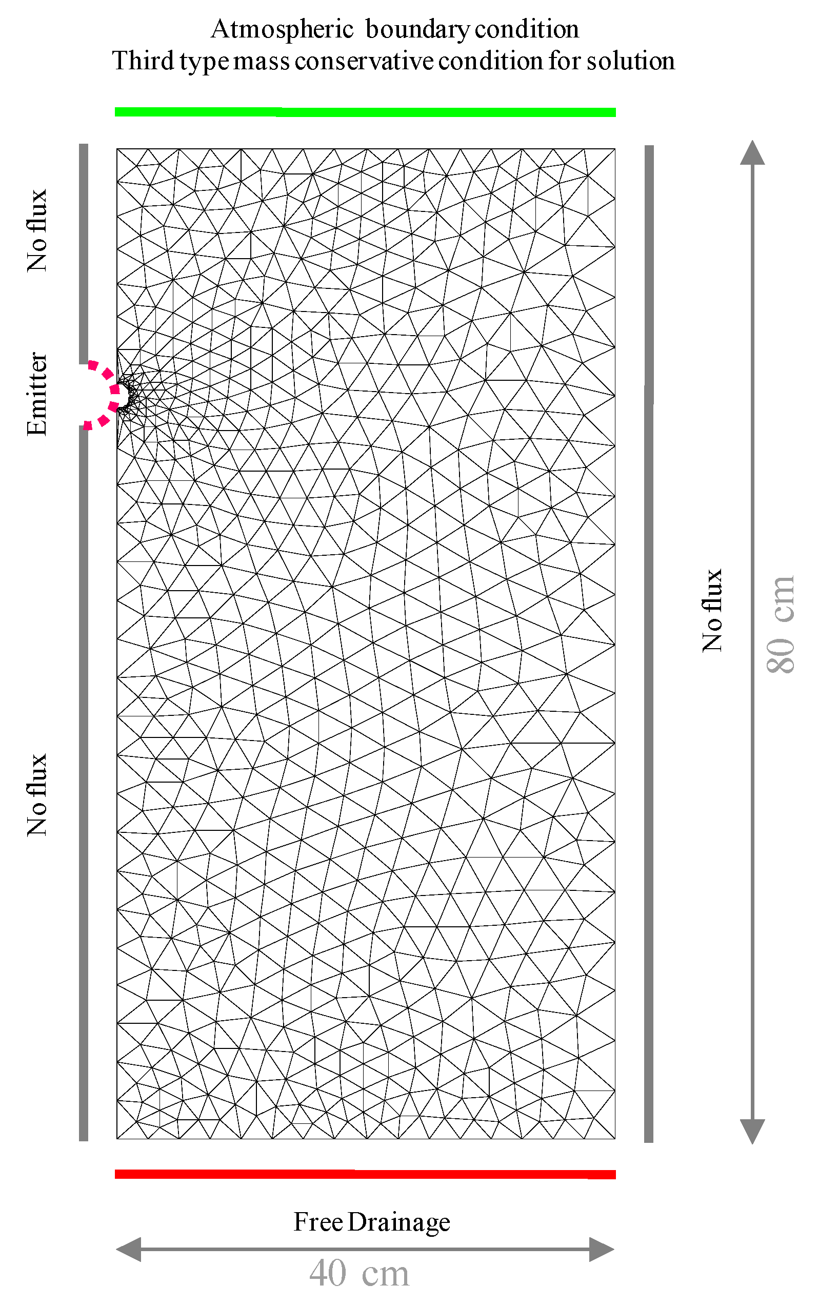
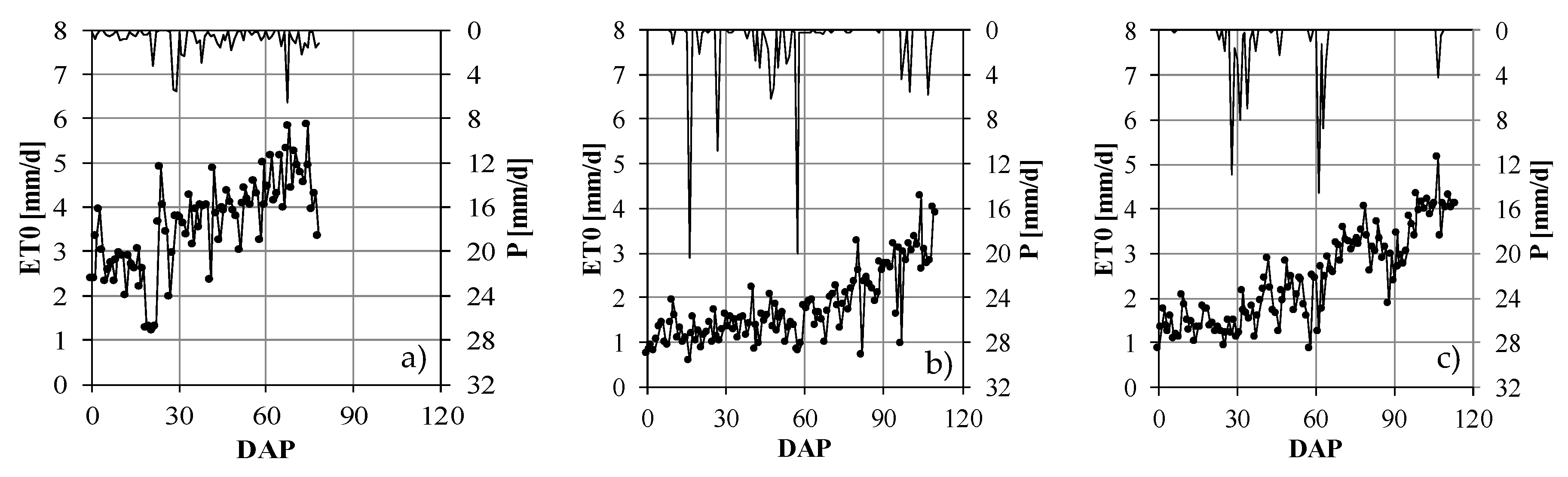
2.1. Experimental Setup and Field Measurements

Experiments were carried out at the High Agronomic Institute of Chott Mariem, Sousse, Tunisia (longitude 10.5632° W; latitude 35.9191° N, altitude 19 m a.s.l.). Potato crop (Solanum Tuberosum L., cv. Safran) was planted during three seasons (spring 2012 and winter 2014 and 2015). Details of vegetative cycle, treatments, field dimensions, and irrigation strategies for the three seasons are summarized in Table 1.
In full irrigation, FI, irrigation volumes restored approximately the maximum crop evapotranspiration estimated between consecutive watering, whereas in deficit irrigation, DI, only half of the volume provided in FI was applied. Irrigation water in treatments T1–T2 was characterized by electrical conductivity ECw = 1.6 dS/m, whereas in treatments T3–T4, it resulted that ECw = 4.2 dS/m. Potatoes were planted at distance of 0.40 m along the row and 0.80 m between the rows and irrigated with a subsurface drip irrigation system with one lateral per plant row, installed at 0.20 m depth. Emitters were spaced 0.40 m and discharged a flow rate of 4.0 l/h at the operating pressure of 130 kPa.
Preliminarily, the flow rate–pressure head relationship, q(h) and the manufacturing coefficient of variation, CV, were evaluated by testing a sample of 25 emitters by following the International Standard 9261:2004,ISO, [37]. The manufacturer coefficient of variation at the examined operating pressure resulted equal to 2.6%, and therefore the emitters’ quality was classified as excellent according to the criterion proposed by Solomon [38]. Daily values of climate variables (solar radiation, minimum and maximum air temperature, relative humidity, and wind speed at 2.0 m height), aimed to compute reference evapotranspiration according to the FAO-56 Penman–Monteith equation [39], were acquired during the growth seasons. Preliminarily, soil physical and hydraulic characteristics were determined on undisturbed soil samples (8.0 cm diameter and 5.0 cm height) collected at three different depths (0–20 cm, 20–40 cm and 40–60 cm). The water column technique performed in Buckner funnels, equipped with porous plates with air entry point h = −200 hPa, was used for matric potentials ranging between 0 hPa (saturation) and about −150 hPa, whereas the pressiometric method using the Richard apparatus was applied for soil matric potential of −330, −1000, −3300, and −15,000 hPa [40]. Saturated hydraulic conductivity was determined, on the same soil samples, by the constant head permeameter. During the investigated seasons, spatial and temporal variability of soil water content around a single emitter, was monitored with a Time Domain Reflectometry (TDR) probe (Trime TDR, IMKO Micromodultechnik GmbH) characterized by a precision of ±0.03 cm3/cm3 [41]. The probe, inserted in plastic access tubes preventively installed, allowed measuring volumetric soil water contents in a soil volume having diameter and height equal to about 15 cm. Three 80 cm long access tubes were installed in each treatment (T1, T2, T3, and T4) perpendicularly to the plant row, at distances of 5, 15, and 40 cm from the emitter. Measurements were acquired each 10 cm of soil depth.
In T3 and T4, soil electrical conductivity was determined on saturated extract (ECe) approximately every 20–25 days according to the method suggested by the US Salinity Laboratory Staff [42] on samples collected at three depths (0–20 cm, 20–40 cm, and 40–60 cm) and two vertical profiles (0 and 25 cm from the emitter). Considering that the method is destructive, each measurement was carried out in correspondence with different emitters.
Crop agronomic parameters, i.e., main root dimensions and leaf surface area, were also measured on three different plants collected at different crop stages from randomly chosen locations of each subplot. In particular, after cleaning the roots, the maximum rooting depth and radius, as well as the depth of maximum density, were measured with a ruler. Then, all the leaves were detached and their surface area measured with the planimetric technique implemented in the Skye Leaf v2 software (Skye Instruments Ltd., Llandrindod Wells, UK). In 2015, additional infrared thermal images were acquired with a thermal camera (HSI3000, Palmer Wahl Instruments Inc., Asheville, NC, USA). The camera thermal sensitivity is approximately of 0.15 °C and the temperature accuracy ranges between ±2 °C and ±2% of the reading in °C. Seven acquisitions were registered in each treatment, from 15 days after plant emergency to seven days before harvesting. In particular, two measurements were acquired during the crop initiation, three at full development stage and two before harvesting. During clear days, thermal images were acquired at midday in the same plants where soil water status were monitored; the camera was fixed at 1.8 m height, by setting the main axes along the vertical. In order to remove the disturbance due to the soil, images were elaborated by the Wahl Heat Spy HSI3000 software and then processed with ENVI 1.4 image analysis software [2], so as to obtain the corresponding weighted average temperature. These latter values were finally used to estimate the crop water stress index (CWSI) after estimating the upper and lower limits with the procedure proposed by Idso et al. [43].
C W S I =   Δ T c a Δ T l Δ T u Δ T l
where ΔTca is the difference between canopy and air temperature (TcTa), ΔTu is the upper limit of TcTa obtained on non-transpiring crops, and ΔTl is the lower limit of TcTa of well-watered crops. A value of CWSI = 0 indicates the absence of stress, whereas a value equal to 1.0 identifies the maximum stress.

2.2. Parametrization and Evaluation of Hydrus-2D Model
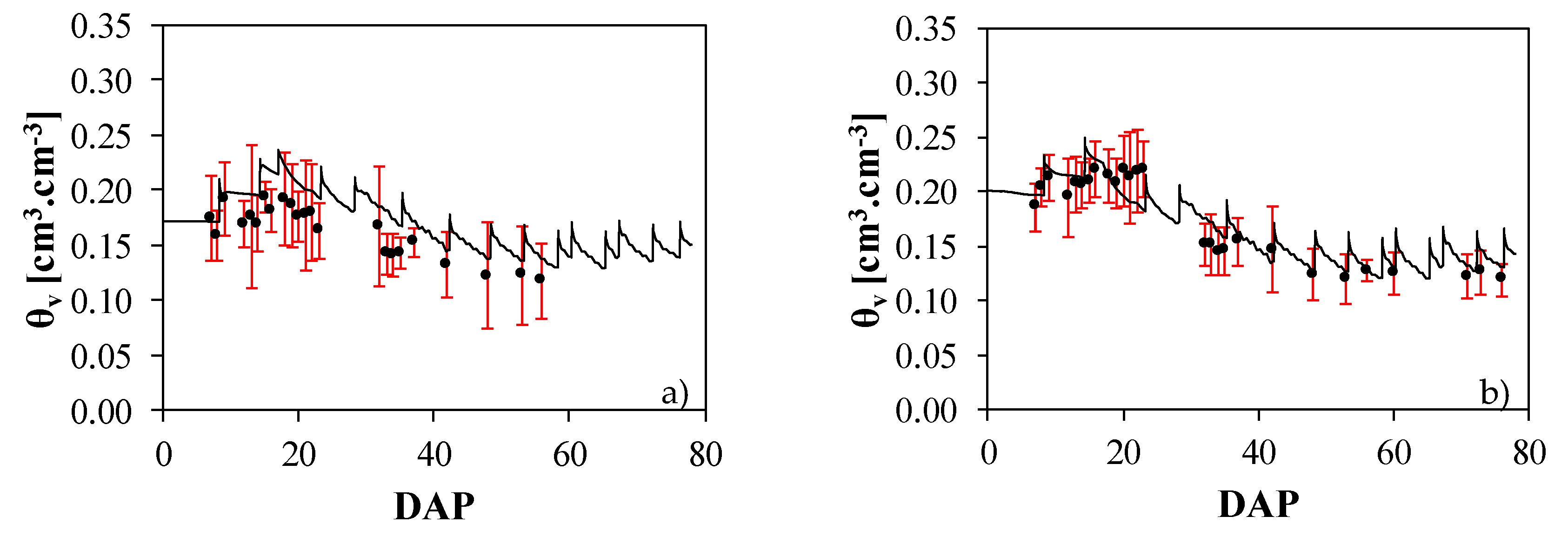
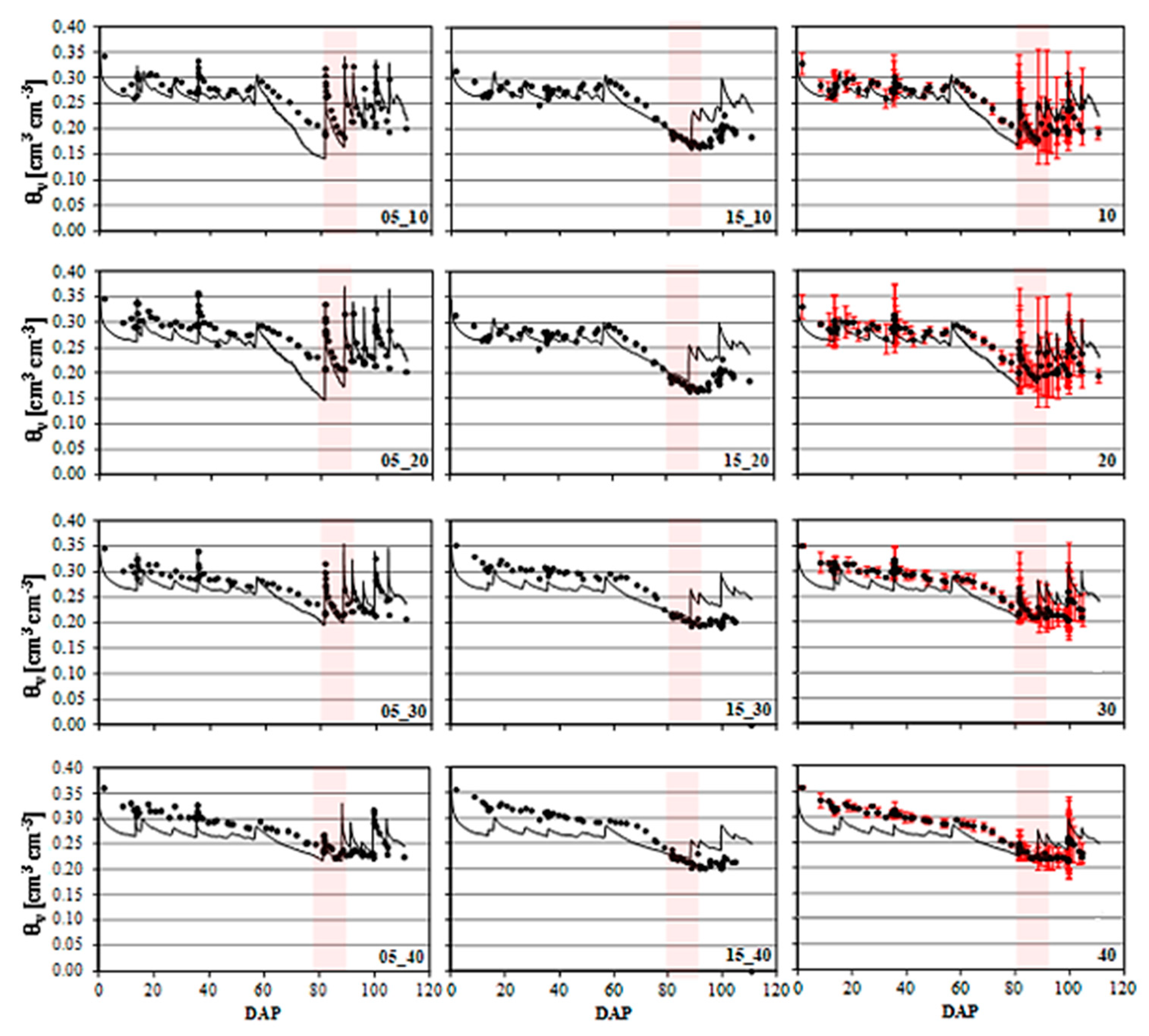
Hydrus-2D model [44] was used to simulate the spatial and temporal dynamic of soil water content and/or soil electrical conductivity for potato crops during the three seasons. Simulations were carried out around a single emitter, on an hourly basis, from the first Day After Planting (DAP) to the end of the crop cycle. Soil hydraulic functions were expressed according to the van Genuchten–Mualem analytical functions [45,46], whose parameters were evaluated based on the measured data. The simulation domain, 80 cm depth and 40 cm wide, was discretized with 721 nodes and 1346 triangular elements, which were detailed around the emitter to account for the fast variations of soil water content during irrigation. Based on the low emitter spacing (0.40 m) it was assumed that at the end of each watering, wetting patterns of consecutive emitters overlapped to a certain extent; following this assumption, infiltration and redistribution processes were schematized according to a two-dimensional vertical plane.
Figure 1 shows the grid and the boundary conditions used for the simulations. The emitter constant flux was obtained by dividing the emitter discharge by the surface of drip pipe as:
q = f l o w   r a t e p i p e   s u r f a c e   a r e a = 4000   cm 3   h 1 2   π   ( 1 cm ) ( 40 cm ) = 15.9   cm   h 1
Even though according to Shani et al. [47] a rising positive back pressure could occur depending on emitter’s flow rate, soil texture, and the dimension of the cavity around the emitter, the assumption of constant flux density is consistent with the high permeability characterizing the investigated soil [48].
The dual crop coefficient approach proposed by FAO [39], based on reference evapotranspiration (ET0) as well as on values of basal crop coefficient Kcb and soil evaporation coefficient, Ke was considered to estimate separately maximum soil evaporation, Emax, and maximum crop transpiration, Tmax. Hydrus-2D considers the modified Feddes model to predict the water response function [49]. Root distribution was schematized according to the Vrugt model [50], whose parameters were estimated based on the measurements acquired in the different phases of growth season. Initial soil water contents were fixed according to the values measured in each treatment at the beginning of the crop cycle. These values were equal to 0.18 and 0.20 cm3 cm−3 for T1 and T3 in 2012 and equal to 0.35, 0.20, 0.30, and 0.30 cm3 cm−3, respectively for T1, T2, T3, and T4 in 2014.
In order to simulate soil salinity, solutes were assumed nonreactive, so that solubilization or dissolution processes were neglected. This assumption allowed the simulation of soil salinity based on the convection–dispersion equation for nonreactive solutes. The measured water electrical conductivity was inputted in the time-dependent boundary condition, so that solute could enter in the system only during irrigation. For all the treatments, the initial salt concentration was assumed equal to the value measured at the beginning of each growing season. At the beginning of simulations, electrical conductivity of soil saturated extract was set equal to 2.5 dS m−1, as measured in the field; this value was converted in salt concentration [g dm−3] by considering a factor of 640 [42]. A third type mass conservative boundary condition was considered for T3 and T4, with solute flux along the emitter boundary equal to 2.56 and 2.05 g dm−3, respectively in 2012 and 2014, obtained according to the measured water electrical conductivity. A multiplicative model was used to account for the combined effects of water and salinity stress [51]. Simulations carried out with Hydrus-2D allowed for the evaluation, on an hourly basis, of the distribution of soil water content and salinity for each node of the considered domain. The performance of the model to simulate soil water content was evaluated based on the Mean Bias Error (MBE), the Root Mean Square Error (RMSE), and the Nash–Sutcliffe efficiency index (NSE). Details on these statistical indicators can be found in the paper of Autovino et al. [52]. In 2012, because of the formation of air gap after around one month in some access tubes, these statistical indicators were calculated only based on the average water contents of the whole soil profile. On the other hand, in 2014 the statistical parameters were calculated based on all the data available at eight different positions (two distances from emitter and four depths) and 60 measurements during the entire growth season. Soil water contents acquired from the farthest access tubes (50 cm from the emitter), as well as those measured at depths deeper than 50 cm, were not considered in the analysis, because these measurements were only marginally affected by irrigation. The paired t test and regression coefficients were used for testing the ability of the model to simulate the electrical conductivity of soil saturated extract (ECe).
For the days of growth season 2015 in which leaf temperatures were measured, the stress coefficient (Ks,meas) was calculated according to the suggestion of Idso et al. [43], as the complement to one of crop water stress index (Ks-meas = 1 − CWSI). These values were used to test the ability of Hydrus-2D to simulate the ratio between actual and maximum transpiration (Ks-sim), which is also related to crop water stress. Once the ability of the model to simulate crop water stress in 2015 was tested, simulations allowed the estimation of transpiration fluxes in 2012 and 2014. Cumulative values of simulated actual and maximum transpiration were used to parameterize the productive function of potato crop, represented by Equation (1). In order to estimate the maximum crop yield (Ymax), the regression line between actual yield and estimated relative transpiration was plotted, so as to obtain the value of Ymax corresponding to Ks-sim = 1.

3. Results

3.1. Soil and Root Characterization for Model Parametrization

Validation of Hydrus-2D model required the preliminary parameterization of soil hydraulic functions, root distribution, and water uptake models, whose parameters are indicated in Table 2. Soil hydraulic functions were analytically expressed by the van Genuchten–Mualem functions [45,46] and the root distribution was defined according to the model proposed by Vrugt et al. [50], whereas the water response function was predicted according to the modified Feddes model [49]. In the different phenological stages, the root parameters were differentiated according to the day after planting (DAP), by assuming a linear root growth. The considered values were estimated according to the measured maximum vertical and horizontal root depths at the different crop growth stages. On the other hand, the parameters of the water uptake model were retrieved by the literature [53].

3.2. Model Simulations

For model application, reference evapotranspiration (ET0) was estimated based on the meteorological data acquired from the climate station, according to the modified FAO Penman–Monteith equation [39]. Figure 2 shows temporal trends of daily ET0, and precipitation, P, during the three examined growth seasons.
Figure 3 shows the daily values of maximum crop transpiration, Tmax, and soil evaporation, Emax, during the examined growth seasons. The values of basal crop coefficient, Kcb, and evaporation coefficient, Ke, are also indicated in the secondary axes of the graphs.
As can be observed, Tmax tends to increase during the crop development stage, to assume an almost stable value around 4.5 mm day−1 in 2012, 2.8 mm day−1 in 2014, and 3.2 mm day−1 in 2015. At the end of the season, the observed decline of Tmax is due to the reductions of Kcb. The evident reductions of Tmax observed at the end of growth season 2012 are also consequent to the relatively higher temperature registered in the period.
Table 3 summarizes the number of precipitation and irrigation events, the cumulated seasonal precipitation, irrigation, reference, and maximum crop evapotranspiration for all the treatments. As can be observed, frequent precipitation events occurred in 2012, even if the seasonal amount was lower than in 2014 and 2015. The cumulative rainfall in 2012 resulted in being slightly lower than 2015, during which rainfall events were concentrated in quite a low number of rainy days. However, the highest value of cumulative rainfall and the lowest value of seasonal reference evapotranspiration occurred in 2014. When observing the trends of reference evapotranspiration, it can be noticed that during the whole season 2012, the values were sensibly higher than the corresponding estimated in 2014 and 2015, as a consequence of the generally higher daily temperature, solar radiation, and wind speed. Moreover, crop yield in treatment T1 in 2014 and 2015 resulted in being equal to 39.1 and 39.0 t/ha respectively, higher than the corresponding value obtained in 2012 (27.4 t/ha).
Table 4 shows in detail the timing of watering and irrigation depth as well as the total water amount provided in treatments T1 ÷ T4 in 2014 and 2015 and introduced in model simulations. The temporal variability of simulated and measured soil water contents for treatments T1 and T3 for the growth season of 2012 is illustrated in Figure 4. Soil water contents are referred to the average in the soil volume controlled by roots, as simulated by the model.
The temporal variability of simulated and measured soil water contents for treatments T1 and T3 for the growth season of 2012 is illustrated in Figure 4. Soil water contents are referred to the average in the soil volume controlled by roots, as simulated by the model. As can be observed in both treatments, simulated soil water contents resulted quite similar to the measured values, even if the model was not able to simulate in 2012 the punctual values of soil water content (data not shown).
Figure 5 illustrates comparisons between measured and simulated soil water contents (SWC) at different positions around the emitter for treatment T1 in 2014. The right column of the figure shows the average soil water contents, whereas the red background indicates the tuber building phase. Similar results were obtained in the same growth season for the other examined treatments.
Table 5 summarizes MBE, RMSE and NSE obtained by comparing simulated and measured soil water contents in the examined treatments in 2012 and 2014.
Model validation was also carried out based on the comparison between simulated soil electrical conductivity with the corresponding measured on soil saturated paste in T3 (2012) and in T3 and T4 (2014). Figure 6 shows the comparison between measured and predicted values of soil electrical conductivity, whose differences resulted in insignificance according to a paired t-test with a probability level α = 0.05. The figure also shows the regression lines and the perfect fitting line (1:1). By separating the data obtained on treatment T3 from those of treatment T4 (data not shown), it was noticed that in the former treatment, the model allowed a better prediction of ECe than in the latter. The reason for the lower accuracy detected in treatment T4 could depend on the inadequacy of the multiplicative model assumed to combine the effects of water and salinity stress on root water uptake.
Thermal images acquired in 2015 allowed for the evaluation of the suitability of the Hydrus-2D model to predict the measured stress coefficient Ks-meas. Once the model was calibrated based on the water content and electrical conductivity of soil saturated extract, it was used to estimate the ratio between actual and maximum crop transpiration (ks-sim), which is also related to the crop water stress. For the days in which leaf temperatures were measured, Figure 7 shows the temporal patterns of simulated and measured Ks respectively, for treatments T1–T2 and T3–T4.
Measured and simulated Ks were then represented in Figure 8 together with the regression lines obtained for treatments T1–T2 and T3–T4. As can be observed, depending on water quality, two different relationships between the examined variables can be identified, as corroborated by the high determination coefficients associated to the fitting lines.
Figure 9a–c shows the cumulative actual and maximum transpiration for the examined treatments in 2012, 2014, and 2015, whereas Figure 10a summarizes the relationships between crop yields obtained during the three seasons and the ratio between the actual simulated and maximum transpiration (Ks-sim). On the other side, Figure 10b illustrates the productive function of potato crop for the examined site. This function represents the relative yield losses (1 − Ya/Ymax) as function of the reductions of relative transpiration obtained when fresh and saline water are used for irrigation.

4. Discussion and Conclusions

Application of physically based models, like Hydrus-2D, requires a detailed description of the soil plant atmosphere (SPA) continuum through complicated deterministic functions (soil water retention curve, conductivity functions, root distribution, and water uptake function). The better the parameterization of the different functions, the higher the performance of the model. Moreover, the knowledge of soil and/or plant water status is crucial during the phase of model validation, in order to assess the model’s ability to simulate water and solute transport. However, under drip irrigation systems, due to the high gradients of soil water and salt content and the distribution of root system after irrigation, it could be quite difficult to identify the position in which to install the measurement probes and then to detect values of SWC representative of the whole root zone. On the other hand, monitoring transpiration fluxes with thermal images allows for overpassing the problems related to root characterization and to water and salt gradients in the root volume. Experiments carried out during the growth seasons 2012 and 2014 allowed for verifying that simulated soil water contents resulted in being quite similar to the measured values, even if the model was not able to simulate in 2012 the punctual values of soil water contents (data not shown). In 2012, after DAP 10, the mean soil water contents in the root zone tended towards a general decrease and to reach a value of about 0.12 cm3 cm−3 at the full development stage, except for local peaks occurring after irrigation. The temporal dynamic of SWCs in 2014 showed a limited variability at the beginning of vegetative growth, until roughly DAP 55, when the crop was at its full development stage, due to the combined effect of rainfall, irrigation, and crop transpiration. After this period, faster reductions of soil water contents were generally observed, as a consequence of the relatively high crop transpiration. The generally low values of SWCs and their continuous decrease, observed in 2012 in T1 and T3, are the result of the delayed sowing time (mid-March), with the contextual high atmospheric demand and ineffectiveness of rainfall (Table 3). In fact, due to the high number of rainy days (Ne = 62), rainfall events, characterized by quite low intensity, wetted only the topsoil. The temporal dynamic of soil water contents in 2014 showed that during the tuber bulking stage (approximately from DAP 80 to DAP 92), the rise of soil water content consequent to the three irrigation events involved only a short distance (about 5 cm) from the emitter. Considering that the analysis of root distribution evidenced that the maximum root radius in that period resulted of about 40 cm, it follows that the small volumes supplied with irrigation allowed to wet only a very limited volume of soil occupied by roots, in which quite a high gradient of SWC occurred. When considering the average soil water contents at the different depth, it can be noticed that the minimum soil water contents in treatments T1 and T3 resulted in being generally higher than the corresponding measured in treatments T2 and T4. However, in all the examined treatments, during the tuber bulking stage, the crop was subject to different levels of water deficit, which were responsible of the observed differences in crop yield (Table 3). When considering the simulated soil water contents, it can be observed that, except for the first two layers of treatment T2, Hydrus-2D is able to fairly accurately reproduce the evolution of the soil water contents at different distances and depths from the emitters. The evident overestimation of soil water content observed in treatment T2 at 10 and 20 cm depth could be ascribed to an imperfect parameterization of the soil hydraulic functions related to the layer, as well as to possible air gaps occurring near the soil surface between the access tube and the surrounding soil [54,55,56]. Moreover, local differences between measured and simulated data can also be detected, mostly related to the end of the growth season. However, it is relevant to notice that while simulated soil water contents are referred to a node of the simulation grid, the measured values represent the average in the soil volume explored by the sensor. In addition, mainly at the end of growth season, tubers of increasing sizes could have occupied the sensing volume, also affecting the measurements. As indicated in Table 5, the values of RMSE were always lower than 0.04 cm3 cm−3 and values of NSE always result as positive, suggesting that there was a substantial agreement between the average soil water contents in the soil layer from 0.1 m to 0.4 m depth and the corresponding values simulated by the model [57]. A slightly better model performance was obtained in treatments T1 and T3 compared to the other two treatments. This difference could be ascribed to the restrictive assumption of considering similar root distributions in all treatments. In fact, due to the different soil water status characterizing the treatments, mainly during the full development stage, it is possible that the plant has extended the roots in the deeper layers, so involving a soil volume larger than the simulated one [58]. Nevertheless, despite the observed local discrepancies, the model, if accurately parameterized, is suitable to predict fairly well the soil water contents at different distances and depths around a buried emitter, even considering the patterns of root water uptake during the whole growth season. The achieved results are in agreement with those observed by Skaggs et al. [59], who evidenced from a comparison between simulated and measured soil water contents under drip irrigation, that Hydrus-2D can be used to predict the patterns of soil water contents around drip emitters, schematized as a linear source.
When considering ECe, a certain discrepancy was observed between simulated and measured values, even if, according to a paired t-test, differences resulted in not being significant at a probability level α = 0.05. A number of factors can explain the high variability observed in both treatments. The first could be related to the gradients of salt concentration in the soil surrounding a buried emitter. In fact, ECe was measured on samples collected along a certain segment of the soil profile in the proximity of different emitters, and therefore the detected value should be referred to a certain volume of soil rather than to a single point, as simulated by the model. In addition, the evolution of root distribution within the soil profile, as well as the variety of the solutes and their possible interactions, may have played an important role in the dynamics of water and salts in the soil profile. By separating the data obtained in treatment T3 from those of T4, it was possible to notice that in the former treatment the model allowed a better prediction of ECe. The reason for the lower accuracy detected in T4 could be attributed to the inadequacy of the multiplicative model assumed to combine the effects of water and salinity stress on root water uptake. A similar degree of variability was found by other researchers [60], even if they observed a certain underestimation of the predicted ECe, compared to the measured values. These Authors ascribed the observed differences to the temporal patterns of roots, as well as to the conservative or not-conservative nature of the solutes and concluded that a better knowledge of the variables affecting water uptake under saline water applications could contribute to improve the simulation results. However, the observed dispersion of simulated values around the perfect fitting line suggests that the model could be considered suitable for predicting the mean values of soil electrical conductivity around a buried emitter and its temporal dynamic.
Evaluating the results of simulations in terms of suitability of the model to simulate water stress conditions, it was verified that trends of Ks-sim generally followed those of measured values, and therefore the model can be considered suitable for identifying the conditions of crop water stress. Depending on the water quality, two different relationships between measured and simulated Ks were obtained, as corroborated by the high determination coefficients associated to the fitting lines.
When analyzing crop yield, it was possible to notice that maximum crop yield resulted in being about 40 t/ha, and for a value of K’s = 0.6, yield resulted in being slightly higher than 20 t/ha (Figure 10a). These results confirm the findings of Ben Mechlia et al. [61] achieved in a similar experiment carried out on potato crop in Tunisia. These authors obtained marketable yield of about 40 t/ha in case of full irrigation and about 20 t/ha under deficit irrigation, when the applied irrigation volume was approximately 60% of maximum crop evapotranspiration. Water productive function evidenced a value of the yield response ky = 1.16 (Figure 10b), slightly higher than the one proposed by Doorenbos and Kassam [26], equal to 1.1. The knowledge of irrigation water productive function is crucial in regions where water resources for agriculture are scarce and deficit irrigation is practiced as a water management strategy aimed at increasing water use efficiency.
The experimental results associated with model simulations can therefore provide useful guidelines for a more sustainable use of irrigation water in countries like Tunisia characterized by semi-arid environments and a limited availability of water. However, the optimal solution cannot disregard local economic evaluations, such as the cost of water and the related benefits achievable to maximize the farmers’ net income.

Author Contributions

Contribute to the paper has to be shared by the Authors in the following way: H.G., A.M. and B.L. collected the experimental data. H.G., G.R. and G.P. elaborated the data and wrote the paper. All the authors contributed to plan the experiments, to build the experimental setup and to revise the final version of the manuscript.

Funding

This research received no external funding from public and private, nor from commercial or not-for-profit sector.

Acknowledgments

The research activity was carried out in the frame of the co-tutel PhD of H.G., who was enrolled in the PhD course “Water-Soil-Environment” at the high Agronomic Institute of Chott Mariem, Sousse, Tunisia, and in the PhD course in “Scienze Agrarie, Forestali ed Ambientali—curriculum Idronomia Ambientale” at University of Palermo, Palermo, Italy.

Conflicts of Interest

The authors declare no conflict of interest.

References

  1. Douh, B.; Boujelben, A. Improving Water Use Efficiency for a sustainable productivity of agricultural systems using subsurface drip irrigation. J. Agric. Sci. Technol. B 2011, 1, 881–888. [Google Scholar]
  2. Ghazouani, H.; Capodici, F.; Ciraolo, G.; Maltese, A.; Rallo, G.; Provenzano, G. Potential of thermal images and simulation models to assess water and salt stress: Application to potato crop in central Tunisia. Chem. Eng. Trans. 2017, 58, 709–714. [Google Scholar] [CrossRef]
  3. Bouksila, F. Sustainability of Irrigated Agriculture under Salinity Pressure—A Study in Semiarid Tunisia. Ph.D. Thesis, Lund University, Lund, Sweden, 2011. [Google Scholar]
  4. Crescimanno, G.; Provenzano, G.; Booltink, H.W.G. The effect of alternating different water qualities on accumulation and leaching of solutes in a mediterranean cracking soil. Hydrol. Proc. 2002, 16, 717–730. [Google Scholar] [CrossRef]
  5. Alagna, V.; Iovino, M.; Bagarello, V.; Mataix-Solera, J.; Lichner, L. Alternative analysis of transient infiltration experiment to estimate soil water repellency. Hydrol. Proc. 2018, 33, 661–674. [Google Scholar] [CrossRef]
  6. FAOSTAT, Statistics Division; Food and Agriculture Organization of the United Nations: Rome, Italy, 2019. Available online: http://www.fao.org/faostat/en/#home (accessed on 10 January 2019).
  7. Chamba, D.; Zubelzu, S.; Juana, L. Energy, cost and uniformity in the design of drip irrigation systems. Biosyst. Eng. 2019, 178, 200–218. [Google Scholar] [CrossRef]
  8. Provenzano, G.; Di Dio, P.; Palau Salvador, G. New computational fluid dynamic procedure to estimate friction and local losses in coextruded drip laterals. J. Irrig. Drain. Eng. 2007, 133, 520–527. [Google Scholar] [CrossRef]
  9. Provenzano, G.; Alagna, V.; Autovino, D.; Juarez, J.M.; Rallo, G. Analysis of geometrical relationships and friction losses in small-diameter lay-flat polyethylene pipes. J. Irrig. Drain. Eng. 2016, 142. [Google Scholar] [CrossRef]
  10. Rallo, G.; Baiamonte, G.; Manzano Juárez, J.; Provenzano, G. Improvement of FAO-56 model to estimate transpiration fluxes of drought tolerant crops under soil water deficit: Application for olive groves. J. Irrig. Drain. Eng. 2014, 140. [Google Scholar] [CrossRef]
  11. Rallo, G.; González-Altozano, P.; Manzano-Juárez, J.; Provenzano, G. Using field measurements and FAO-56 model to assess the eco-physiological response of citrus orchards under regulated deficit irrigation. Agric. Water Manag. 2017, 180, 136–147. [Google Scholar] [CrossRef]
  12. Bowen, W.T. Water productivity and potato cultivation. In Water Productivity in Agriculture: Limits and Opportunities for Improvement; Kijne, J.W., Barker, R., Molden, D., Eds.; CAB International: Wallingford, UK, 2003; pp. 229–238. [Google Scholar]
  13. Camp, C.R. Subsurface drip irrigation: A review. Trans. Am. Soc. Agric. Eng. 1998, 41, 1353–1367. [Google Scholar] [CrossRef]
  14. Ayars, J.; Schoneman, R.A.; Dale, F.; Meso, B.; Shouse, P. Managing subsurface drip irrigation in the presence of shallow groundwater. Agric. Water Manag. 2001, 47, 243–264. [Google Scholar] [CrossRef]
  15. Provenzano, G.; Rodriguez-Sinobas, L.; Roldán-Cañas, J. Irrigated agriculture: Water resources Managment for a sustainable environment. Biosyst. Eng. 2014, 128, 1–3. [Google Scholar] [CrossRef]
  16. Rodriguez-Sinobas, L.; Provenzano, G.; Roldán-Cañas, J. Special issue: Water Management strategies in irrigated areas. Agric. Water Manag. 2016, 170, 1–4. [Google Scholar] [CrossRef]
  17. Foti, S.; Mauromicale, G.; Ierna, A. Influence of irrigation levels on growth and yield of potato cv. Spunta. Potato Res. 1995, 38, 307–318. [Google Scholar] [CrossRef]
  18. Fabeiro, C.; Martin de Santa Olalla, F.; De Juan, J.A. Yield and size of deficit irrigated potatoes. Agric. Water Manag. 2001, 48, 255–266. [Google Scholar] [CrossRef]
  19. Kayshap, P.S.; Panda, R.K. Effect of irrigation scheduling on potato crop parameters under water stressed conditions. Agric. Water Manag. 2002, 59, 49–66. [Google Scholar] [CrossRef]
  20. Yuan, B.Z.; Nishiyama, S.; Kang, Y. Effects of different irrigation regimes on the growth and yield of drip-irrigated potato. Agric. Water Manag. 2003, 63, 153–167. [Google Scholar] [CrossRef]
  21. Onder, S.; Caliskan, M.E.; Onder, D.; Caliskan, S. Different irrigation methods and water stress effects on potato yield and yield components. Agric. Water Manag. 2005, 73, 73–86. [Google Scholar] [CrossRef]
  22. Wright, J.L.; Stark, J.C. Potato. In Irrigation of Agricultural Crops—Agronomy; Stewart, B.A., Nielsen, D.R., Eds.; Monograph No. 30; ASA-CSSA-SSSA: Madison, WI, USA, 1990. [Google Scholar]
  23. Shock, C.C.; Holmes, Z.A.; Stieber, T.D.; Eldredge, E.P.; Zhang, P. The effect of timed water stress on quality, total solids and reducing sugar content of potatoes. Am. Potato J. 1993, 70, 227–241. [Google Scholar] [CrossRef]
  24. Eldredge, E.P.; Holmes, Z.A.; Mosley, A.R.; Shock, C.C.; Stieber, T.D. Effects of transitory water stress on potato tuber stem-end reducing sugar and fry color. Am. Potato J. 1996, 73, 517–530. [Google Scholar] [CrossRef]
  25. Stewart, J.I.; Hagan, R.M.; Pruitt, W.O.; Danielson, R.E.; Franklin, W.T.; Hanks, R.J.; Riley, J.P.; Jackson, E.B. Optimizing crop production through control of water and salinity levels in the soil. In Reports Paper 67; Utah Water Research Laboratory: Logan, UT, USA, 1977; p. 191. [Google Scholar]
  26. Doorenbos, J.; Kassam, A.H. Yield Response to Water; FAO Irrigation and Drainage Paper No. 33; FAO: Rome, Italy, 1979. [Google Scholar]
  27. Paredes, P.; Rodrigues, G.C.; Alves, I.; Pereira, L.S. Partitioning evapotranspiration, yield prediction and economic returns of maize under various irrigation management strategies. Agric. Water Manag. 2014, 135, 27–39. [Google Scholar] [CrossRef]
  28. Martínez-Gimeno, M.A.; Bonet, L.; Provenzano, G.; Badal, E.; Intrigliolo, D.S.; Ballester, C. Assessment of yield and water productivity of clementine trees under surface and subsurface drip irrigation. Agric. Water Manag. 2018, 206, 209–216. [Google Scholar] [CrossRef]
  29. Manickavasagan, A.; Jayas, D.S.; White, N.D.G.; Paliwal, J. Applications of thermal imaging in agriculture—A Review. In Proceedings of the CSAE/SCGR 2005 Meeting, Winnipeg, MB, Canada, 26–29 June 2005. Paper no. 05-002. [Google Scholar]
  30. Jackson, R.D. Canopy temperature and crop water stress. In Advances in Irrigation; Hillel, D.I., Ed.; Academic Press: Cambridge, MA, USA, 1982; Volume 1, pp. 43–85. [Google Scholar]
  31. Idso, S.B. Non-water-stressed baselines: A key to measuring and interpreting plant water stress. Agric. Meteorol. 1982, 27, 59–70. [Google Scholar] [CrossRef]
  32. Rallo, G.; Agnese, C.; Minacapilli, M.; Provenzano, G. Assessing AQUACROP water stress function to evaluate the transpiration reductions of olive mature tree. Ital. J. Agrometeorol. 2012, 17, 21–28. [Google Scholar]
  33. Rallo, G.; Agnese, C.; Minacapilli, M.; Provenzano, G. Comparison of SWAP and FAO agro-hydrological models to schedule irrigation of wine grapes. J. Irrig. Drain. Eng. 2012, 138, 581–591. [Google Scholar] [CrossRef]
  34. Lazarovitch, N.; Warrick, A.W.; Furman, A.; Šimůnek, J. Subsurface water distribution from drip irrigation described by moment analyses. Vadose Zone J. 2007, 6, 116–123. [Google Scholar] [CrossRef]
  35. Provenzano, G. Using Hydrus-2D simulation model to evaluate wetted soil volume in subsurface drip irrigation systems. J. Irrig. Drain. Eng. 2007, 133, 342–349. [Google Scholar] [CrossRef]
  36. Mguidiche, A.; Provenzano, G.; Douh, B.; Khila, S.; Rallo, G.; Boujelben, A. Assessing Hydrus-2D to simulate soil water content (SWC) and salt accumulation under an SDI system: Application to a potato crop in a semi-arid area of central Tunisia. Irrig. Drain. 2015, 64, 263–274. [Google Scholar] [CrossRef]
  37. International Standard Organization (ISO). Agricultural Irrigation Equipment-Emitters and Emitting Pipes-Specification and Test Methods; ISO 9261:2004(E); International Standard Organization (ISO): Geneva, Switzerland, 2004. [Google Scholar]
  38. Solomon, K.H. Manufacturing variation of emitters in trickle irrigation systems. Trans. ASAE 1979, 22, 1034–1038. [Google Scholar] [CrossRef]
  39. Allen, R.G.; Pereira, L.S.; Raes, D.; Smith, M. Crop Evapotranspiration: Guidelines for Computing Crop Water Requirements; FAO Irrigation and Drainage Paper 56; Food and Agriculture Organization of the United Nations: Rome, Italy, 1998. [Google Scholar]
  40. Dane, J.H.; Hopmans, J.W. Pressure plate extractor. In Methods of Soil Analysis. Part 4. Physical Methods; Dane, J.H., Topp, G.C., Eds.; SSSA Book Ser. 5; SSSA: Madison, WI, USA, 2002; pp. 688–690. [Google Scholar]
  41. Douh, B. Etude Théorique et Expérimentale de L’irrigation Goutte à Goutte Souterraine Sur une Culture de Maïs (Zea mays L.). Ph.D. Thesis, Higher Agronomic Institute of Chott Meriem, Sousse, Tunisia, 2012; 210p. [Google Scholar]
  42. U.S. Salinity Laboratory Staff. Diagnosis and Improvement of Saline and Alkali Soils; USDA, Handbook 60; U.S. Government Printing Office: Washington, DC, USA, 1954.
  43. Idso, S.B.; Jackson, R.D.; Pinter, P.J.; Reginato, R.J.; Hatfield, J.L. Normalizing the stress-degree-day parameter for environmental variability. Agric. Meteorol. 1981, 24, 45–55. [Google Scholar] [CrossRef]
  44. Šimůnek, J.; Šejna, M.; van Genuchten, M.T. The Hydrus-2D Software Package for Simulating Two-Dimensional Movement of Water, Heat, and Multiple Solutes in Variably Saturated Media; Version 2.0, IGWMC-TPS-53; International Ground Water Modeling Center, Colorado School of Mines: Golden, CO, USA, 1999; 251p. [Google Scholar]
  45. Mualem, Y. A new model for predicting the hydraulic conductivity of unsaturated porous media. Water Resour. Res. 1976, 12, 513–522. [Google Scholar] [CrossRef]
  46. van Genuchten, M.T. A closed-form equation for predicting the hydraulic conductivity of unsaturated soils. Soil Sci. Soc. Am. J. 1980, 44, 892–898. [Google Scholar] [CrossRef]
  47. Shani, U.; Xue, S.; Gordin, K.R.; Warrick, A.W. Soil limiting flow from subsurface emitters. I: Pressure measurements. J. Irrig. Drain. Eng. 1996, 122, 291–295. [Google Scholar] [CrossRef]
  48. Provenzano, G. Closure to “Using Hydrus-2D simulation model to evaluate wetted soil volume in subsurface drip irrigation systems”. J. Irrig. Drain. Eng. 2008, 134, 878–879. [Google Scholar] [CrossRef]
  49. Feddes, R.A.; Kowalik, P.J.; Zaradny, H. Simulation of Field Water Use and Crop Yield; Simulation Monographs; PUDOC: Wageningen, The Netherlands, 1978; 189p. [Google Scholar]
  50. Vrugt, J.A.; van Wijk, M.T.; Hopmans, J.W.; Šimůnek, J. One-, two-, and three dimensional root water uptake functions for transient modeling. Water Resour. Res. 2001, 37, 2457–2470. [Google Scholar] [CrossRef]
  51. Skaggs, T.H.; van Genuchten, M.Th.; Shouse, P.J.; Poss, J.A. Macroscopic approaches to root water uptake as a function of water and salinity stress. Agric. Water Manag. 2006, 86, 140–149. [Google Scholar] [CrossRef]
  52. Autovino, D.; Rallo, G.; Provenzano, G. Predicting soil and plant water status dynamic in olive orchards under different irrigation systems with Hydrus-2D: Model performance and scenario analysis. Agric. Water Manag. 2018, 203, 225–235. [Google Scholar] [CrossRef] [Green Version]
  53. Wesseling, J.G.; Elbers, J.A.; Kabat, P.; van den Broek, B.J. SWATRE: Instructions for Input; Internal Note; Winand Staring Centre: Wageningen, The Netherlands, 1991. [Google Scholar]
  54. Rallo, G.; Provenzano, G. Discussion of “Laboratory and Field Calibration of the Diviner 2000 Probe in Two Types of Soil”. J. Irrig. Drain. Eng. 2014, 141. [Google Scholar] [CrossRef]
  55. Rallo, G.; Agnese, C.; Blanda, F.; Minacapilli, M.; Provenzano, G. Agro-Hydrological models to schedule irrigation of Mediterranean tree crops. Ital. J. Agrometeorol. 2010, 1, 11–21. [Google Scholar]
  56. Ghazouani, H.; Autovino, D.; Rallo, G.; Douh, B.; Provenzano, G. Using Hydrus-2D model to assess the optimal drip lateral depth for Eggplant crop in a sandy loam soil of central Tunisia. Ital. J. Agrometeorol. 2016, 1, 47–58. [Google Scholar] [CrossRef]
  57. Nash, J.E.; Sutcliffe, J.V. River flow forecasting through conceptual models: Part 1. A discussion of principles. J. Hydrol. 1970, 10, 282–290. [Google Scholar] [CrossRef]
  58. Phogat, V.; Skewes, M.A.; Cox, J.W.; Sanderson, G.; Alam, J.; Šimůnek, J. Seasonal simulation of water, salinity, and nitrate dynamics under drip irrigated mandarin (Citrus reticulata) and assessing management options for drainage and nitrate leaching. J. Hydrol. 2014, 513, 504–516. [Google Scholar] [CrossRef]
  59. Skaggs, T.H.; Trout, T.J.; Šimůnek, J.; Shouse, P.J. Comparison of Hydrus-2D simulations of drip irrigation with experimental observations. J. Irrig. Drain. Eng. 2004, 130, 304–310. [Google Scholar] [CrossRef]
  60. Roberts, T.; Lazarovitch, N.; Warrick, A.W.; Thompson, T.L. Modeling salt accumulation with subsurface drip irrigation using Hydrus-2D. Soil Sci. Soc. Am. J. 2009, 73, 233–240. [Google Scholar] [CrossRef]
  61. Ben Mechlia, N.; Nagaz, K.; Abid-Karray, J.; Masmoudi, M.M. Productivity of the potato crop under irrigation with low quality waters. In Water Use Efficiency and Water Productivity: WASAMED Project; Options Méditerranéennes: Série B. Etudes et Recherches; n. 57; Lamaddalena, N., Shatanawi, M., Todorovic, M., Bogliotti, C., Albrizio, R., Eds.; CIHEAM: Bari, Italy, 2007; pp. 205–210. [Google Scholar]
Figure 1. Grid used for Hydrus-2D simulations and related boundary conditions.
Water 11 00540 g001
Figure 2. Trends of daily reference evapotranspiration, ET0, and precipitation, P, during 2012 (a), 2014 (b) and 2015 (c).
Water 11 00540 g002
Figure 3. (ac) Daily maximum crop transpiration, Tmax, and soil evaporation, Emax, during growth seasons 2012, 2014 and 2015. Basal crop coefficient, Kcb, and evaporation coefficient, Ke, are indicated in the secondary axes.
Water 11 00540 g003
Figure 4. Temporal variability of average simulated (solid line) and measured (black dots) soil water contents (SWCs) in the root zone for treatments T1 (a) and T3 (b) during the growth season of 2012. Standard deviations of measured SWCs are indicated with red bars.
Water 11 00540 g004
Figure 5. Comparison between measured (black dots) and simulated (solid line) soil water contents (SWCs), θv, in treatment T1 (2014) at depths 10, 20, 30, and 40 cm and distances of 5 and 15 cm from the emitter. Red background indicates the tuber building phase. Average values are shown in the right column.
Water 11 00540 g005
Figure 6. Simulated and measured mean soil electrical conductivity obtained in (a) 2012 in treatment T3, and (b) 2014 in treatments T3 and T4.
Water 11 00540 g006
Figure 7. (a,b) Temporal dynamic of measured (dots) and simulated Ks (continuous curve) obtained in 2015. The red lines identify the phase from tuber initiation to the end of tuber formation.
Water 11 00540 g007
Figure 8. Relationships between measured and simulated Ks.
Water 11 00540 g008
Figure 9. Temporal dynamic of cumulative actual and maximum transpiration for the examined treatments in 2012 (a), 2014 (b), and 2015 (c).
Water 11 00540 g009
Figure 10. Yield as a function of the simulated stress coefficient, Ks-sim (a), and the productive function of potato crop (b).
Water 11 00540 g010
Table 1. Crop cycle, treatments and related water quality, field dimensions and irrigation strategies applied during the three investigated seasons.
YearCrop CycleTreatmentsECw 1Field DimensionsIrrigation Strategy 2
[dS m−1][m × m]
2012March, 14th to June, 1stT11.6 25 × 15.0FI
T34.225 × 15.0FI
2014January, 15th to May, 6thT11.6 25 × 7.5FI
T21.6 25 × 7.5DI
T34.2 25 × 7.5FI
T44.2 25 × 7.5DI
2015January, 22nd to May, 17thT11.6 25 × 7.5FI
T21.6 25 × 7.5DI
T34.2 25 × 7.5FI
T44.2 25 × 7.5DI
1 ECw: Electrical conductivity of irrigation water; 2 FI: Full irrigation, DI: Deficit irrigation.
Table 2. Summary of parameters for soil hydraulic functions, root distribution and water uptake models used in simulations.
Soil Hydraulic Functions 1
θsθrαnmK0λ
[cm3 cm−3][cm3 cm−3][cm−1][-][-][cm h−1][-]
0.390.080.011.590.377.10.5
Root Distribution Model 2
ZmaxRmaxZ*R*
DAP[cm][cm][cm][cm]
20120–4040201810
40–5145302015
51–7550402218
20140–2423201510
24–7844352020
78–10950402020
20150–2923201510
29–8344352020
83–11350402020
Water Uptake Model 3
P0PoptP2HP2LP3r2Hr2L
[kPa][kPa][kPa][kPa][kPa][cm d−1][cm d−1]
−1.0−2.5−30−80−16000.010.002
1 θs and θr are the saturated and residual water contents; α is related to the inverse of the air-entry pressure; n and m parameters with m = 1 − 1/n; K0 is the saturated hydraulic conductivity; λ is an empirical pore-connectivity parameter. 2 Zmax and Rmax are the maximum rooting depth and radius, Z* and R* are the locations of the maximum root water uptake in the vertical and horizontal directions. 3 P0 is the pressure head below which roots extract water from the soil; Popt is pressure head below which roots extraction is maximum; P2H is the limiting pressure head below which roots extraction is lower than the potential transpiration rate (r2H); P2L is limiting pressure head below which roots no longer extract water at the potential transpiration rate (r2L); P3 is the pressure head below which root water uptake ceases.
Table 3. Number of precipitation events (Ne) and irrigation watering (Ni), seasonal precipitation (P) and irrigation (I), reference evapotranspiration (ET0), maximum evapotranspiration (ETmax), mean (μ) and standard deviation (σ) of crop yield, for the examined treatments in 2012, 2014 and 2015.
NeNiPIET0ETmaxYield
[-][-][mm][mm][mm][mm][t/ha]
μσ
2012
T1621465.2175.0286.5224.727.42.3
T3621465.2175.0286.5224.725.92.1
2014
T1408108.6124.4198.0160.1739.18.3
T2408108.661.1198.0160.1724.910.7
T3407108.6112.2198.0160.1724.19.4
T4407108.667.1198.0160.1719.513.3
2015
T1211473.6181.9280.0221.039.0 8.3
T2211473.694.5280.0221.025.83.2
T3211473.6165.1280.0221.026.39.4
T4211473.683.1280.0221.016.32.4
Table 4. Water amount [mm] provided during each irrigation event in 2014 and 2015.
DateT1T2DateT3T4
201429 January 20149.44.828 January201415.59.2
20 February 201411.56.419 February 20149.95.4
7 April 201412.95.18 April 201413.67.3
14 April 201428.27.111 April 201427.917.6
17 April 201414.58.518 April 201418.812.6
21 April 20145.68.324 April 201415.29.9
25 April 201430.114.730 April 201411.35.1
30 April 201412.26.3
Total124.461.1Total112.267.1
201527 January 201511.86.627 January 20157.84.1
5 February 201511.86.85 February 201512.68.1
12 February 20157.23.612 February 20157.35.3
19 March 201511.46.519 March 20158.15.3
4 April 201510.55.34 April 20159.14.7
10 April 201516.48.410 April 201522.77.0
21 April 201512.16.221 April 201510.55.2
24 April 201513.36.824 April 201511.65.7
29 April 201515.37.729 April 201513.26.6
1 May 201518.29.31 May 201515.87.9
4 May 201514.07.14 May 201512.16.0
8 May 201515.57.98 May 201513.56.7
12 May 20158.94.512 May 20157.83.9
15 May 201515.47.715 May 201513.36.6
Total181.894.4Total165.183.1
Table 5. Statistical parameters used to assess the performance of Hydrus-2D to simulate soil water contents (SWC).
All MeasurementsAverage
Mean Bias Error (MBE)Root Mean Square Error (RMSE)Nash–Sutcliffe Efficiency Index (NSE)MBERMSENSE
[cm3 cm−3][ cm3 cm−3][-][cm3 cm−3][ cm3 cm−3][-]
2012
T1 0.030.010.48
T3 0.030.030.45
2014
T1−0.110.020.49−0.010.010.60
T20.030.030.290.040.030.28
T30.010.040.400.010.030.50
T40.020.030.350.010.020.57

