Assessment of the Decadal Impact of Wildfire on Water Quality in Forested Catchments

Abstract

Wildfire can have significant impacts on hydrological processes in forested catchments, and a key area of concern is the impact upon water quality, particularly in catchments that supply drinking water. Wildfire effects runoff, erosion, and increases the influx of other pollutants into catchment waterways. Research suggests that suspended sediment and nutrient levels increase following wildfire. However, past studies on catchment water quality change have generally focused on the short term (1–3 years) effects of wildfire. For appropriate catchment management, it is important to know the long-term effect of wildfire on catchment water quality and the recovery process. In this study, a statistical analysis was performed to examine the effect of 2001/2002 Sydney wildfire on catchment water quality. This research is particularly important, since the catchments studied provide drinking water to Sydney. Linear mixed models were used in this study in an analysis of covariance (ANCOVA)-type change detection approach to assess the effect of wildfire. We used both burnt and unburnt catchments to aid the interpretation of the results and to help disentangle the effects of natural climate variation, as well as of the wildfire. The results of this study showed persistent long-term (10-year) effects of wildfire, including increases in total suspended sediment concentrations (64% higher than in unburnt catchments), total nitrogen concentrations (48% higher), and total phosphorus (40% higher).

1. Introduction

Wildfire can have a significant impact on the hydrologic cycle of forested catchments due to changes in the surface vegetation and canopy cover, combined with ash sealing of soil pores [1,2]. This is of particular concern for water quality (WQ) in forested catchments [3,4], as in many cases these catchments supply drinking water to urban communities [5]. The frequency of wildfire is expected to increase due to climate change [6]. In response, there has been an increase in the number of studies on the effect of wildfire on catchment hydrology [7,8,9]. Suspended sediment and nutrients (phosphorus and nitrogen) are two important measures of catchment water quality [10]. Increases in total suspended sediment (TSS) in rivers limits light penetration, hampering primary productivity within the river [11]. Increases in total phosphorus (TP) and total nitrogen (TN) levels can result in excessive algal growth [12].

Increases in TSS and nutrient levels arise from the effects of wildfire on erosion, runoff, infiltration, and the combustion of organic matter. When a catchment is burnt the wildfire removes surface vegetation, which increases the percentage of rainfall available for runoff. Furthermore it decreases evapotranspiration, which increases overland flow, and subsequently the amount of flow in streams [13]. These conditions promote higher levels of soil erosion. Erosion can also be driven by the reduction in infiltration as ash seals, soil pores and soil heating produces hydrophobic soil layers [14,15,16]. Additionally, during a wildfire, burning and heating of organic matter releases charcoal, ash, heavy metals and other stable nutrients that might be previously unavailable for transport into waterways [17].

Table 1. Past Studies on wildfire effect on WQ.

Study	Description	Pre-Wildfire Data/Post-Wildfire Data	Method 1	Limitation
Lane, Sheridan and Noske [7]	Severe wildfire burnt over 1 million ha of forested land in Australia	10 years/2 years post-wildfire	ANCOVA (with control) 2	Long term impact were hard to compare due to the high variations in climate and the effect of logging.
Bladon, Silins, Wagner, Stone, Emelko, Mendoza, Devito and Boon [19]	The effect of wildfire on post-wildfire nitrogen concentration with 3 burnt catchments and 2 unburnt catchments	NA/3 years	ANCOVA (with control)	Lack of pre-wildfire WQ data and there is a shortage in assessing the initial wildfire effect on WQ and recovery of the catchments.
Mast and Clow D.W [28]	Post-wildfire WQ change after a wildfire in Glacier National Park, USA	5 years/4 years	Compare average concentration	No control (unburnt) catchment studed. Result effected by snow melt event (first flow released during long period of time).
Townsend and Douglas [12]	The effect of a wildfire on stream WQ and catchment water yield in a tropical savanna (North Australia) excluded from wildfire for 10 years	3 years/10th year post-wildfire	ANCOVA (No control)	Only the WQ 10 years post-wildfire was described, no earlier observation was compared with pre-wildfire data.
Malmon, et al. [29]	Sediment change post-wildfire in New Mexico	2 years/3 years	ANCOVA (No control)	Only 2 years pre-wildfire data was used in the study.
Kunze and Stednick [30]	Sediment change post-wildfire in 2 burnt catchments in Colorada, USA.	NA/3 years	ANCOVA (with control)	No available pre-wildfire data. First year post-wildfire, WQ and quantity data were collected only after events.
Oliver, Reuter, Heyvaert and Dahlgren [20]	Analyisis the WQ change post a severe wildfire in lake Tahoe basin, USA	10 years/2 years	ANCOVA	Pre-wildfire sample collected monthly and during events, no information on daily or annual discharge.
Hauer and Spencer [31]	Phosphorus and nitrogen concentration change after wildfire in Columbia	NA/5 years	Compare average concentration	Lack of pre-wildfire data Limited data were collected at some sites due to funding limit.

¹ ANCOVA method: using regression model to account for the effect of flow on WQ. ² Unburnt catchment is used as a control, the pre- and post-wildfire WQ and quantity change are compared.

presents a summary of studies that assessed the impact of wildfire on WQ with a focus on TSS, TP, and TN. Most only examined the effects 1–4 years post-wildfire, which identifies a gap in knowledge about the long term impacts. This is especially important given that some studies have shown wildfire can impact flow for decades post-wildfire [18]. Challenges facing long-term wildfire research are centered around the lack of pre-wildfire water quality data, and more generally the need for fine-scale spatial and temporal data both before and after the wildfire to increase the sensitivity of change detection approaches. Shakesby and Doerr [1] identified that aforementioned lack of pre-wildfire data as a major problem in relating post-wildfire erosion rates to long term conditions. In some studies such as [19], they were unable to compare their catchment state with catchment pre-wildfire conditions due to the absence of pre-wildfire WQ data. The exception is Lane, Sheridan and Noske [7] and Oliver, et al. [20], who both had long term pre-wildfire data. In terms of assessing the impacts of wildfire on WQ, both a long pre-wildfire and post-wildfire dataset is required.

Another issue with past studies is the nature of sampling in terms of how well they represent the variation in WQ, which also relates to the validity of the statistical models fitted to the data to assess change. For example, Oliver, et al. [20] indicated their pre-wildfire WQ data were collected on a monthly time step, and occasionally during an event. This is a common method used in most catchments’ WQ monitoring programs [21] due to the high cost of environmental sampling. Past work has shown that monthly sampling does not reflect the range of hydrological conditions in a catchment, especially over the short term [22].

In order to detect change, least-square regression is used to fit a regression model of some form in nearly all cases. However this assumes the data has been collected using a probabilistic sampling design, which in this context involves randomization of the sample times. This allows us to assume that the observations are independent, and this makes a least-squares model fitting valid. However, in the studies in Table 1, the fixed interval sampling or event-based sampling is not randomized. Therefore, we need to account for potential auto-correlation by using model-based approaches as exemplified by linear mixed models (LMM) [23]. This approach calculates an unbiased estimate of the variances, and allows statistically valid hypothesis testing which is crucial in change detection studies.

In terms of detecting WQ change a typical approach is to account for differences in discharge between pre- and post-wildfire periods, with an analysis of covariance (ANCOVA) model, which compares two regression lines to detect whether there is a difference between the model parameters; e.g. slope, for the pre- and post-wildfire periods [24,25]. Alternatively, a paired approach may be adopted where a neighboring unburnt catchment is used. During the pre-wildfire period a regression model between WQ from these two catchments is created, the model is then used to predict the burnt catchment’s WQ for the post-wildfire period. The observed prediction error indicates a possible wildfire effect. Importantly, a paired study requires high similarities between the paired catchments in terms of slope, soil, land use and climate conditions. An issue with this approach, and an ANCOVA, is that the regression model which uses discharge only to model WQ may be overly simplistic, and does not represent antecedent conditions and hysteresis, i.e., rising/falling limbs, which control the discharge-WQ relationship [26].

Additionally, most past studies (such as studies mentioned above) used empirical models for water quality predicting and monitoring, this process ignored the topographic differences e.g., soil, topography, in the modeling process [27]. However, these models require high level of input spatial and climate data, which is not always available for most studies. Thus, this method is not discussed in this study.

In summary, gaps in existing research are:

• Lack of studies showing >5 years post-wildfire impact on WQ;
• lack of studies with adequate pre- and post-wildfire data;
• past studies predominantly use least-square regression models for change detection without accounting for auto-correlation in the data, and therefore hypothesis testing is erroneous;
• past studies rely on simple discharge-WQ models to detect change due to wildfire.

The 2001/2002 wildfires around Sydney provide an opportunity to address all of these issues due to the fact that they were widespread and predominantly in water supply catchments, meaning that the pre- and post-wildfire WQ data was numerous. More specifically this work aims to:

• Assess the medium-term impacts of wildfire on WQ in the forest catchments around Sydney based on a 10 years pre-wildfire and 10 years post-wildfire dataset;
• present an approach using LMM to detect change based on sparse (as compared to discharge) WQ observations to address the shortcomings identified previously.

2. Materials and Methods

2.1. Study Area

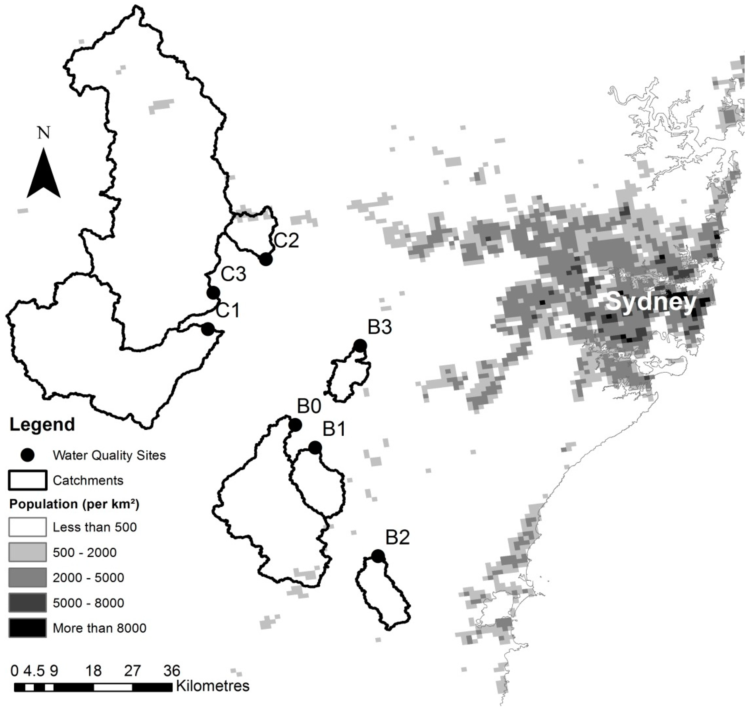
In the period between 3 December 2001 and 14 January 2002, wildfire burnt an area of approximately 7333 km² (2831 m²) around Sydney, Australia [32]. Much of the area burnt was located in the catchment area of Lake Burragorang, which is impounded by Warragamba Dam. It provides 80% of Sydney’s drinking water, and within the catchment there are approximately 200,000 residents [33]. Due to its importance, many streams in the area are monitored for water quality by a government agency, WaterNSW, and have WQ measurements before and after the wildfire. The criteria used to select monitoring stations include: Have adequate WQ data pre- and post-wildfire, and also have extensive forest cover (>65%) in the catchment area above each monitoring station, which yielded a total of seven monitoring stations. These criteria were used here because the focus of this work is the impact of wildfire on the WQ of forested catchments. The location of the seven catchments is presented in Figure 1, where four catchments were unburnt (control) and 3 catchments were burnt.

The four burnt catchments have an area ranging from 56 km² to 436 km², had forest cover from 69–97% pre-wildfire, and annual rainfall ranged from 694 mm to 1182 mm. The three unburnt catchments have areas that range from 72 km² to 1447 km², had forest cover from 73–90% pre-wildfire, and annual rainfall range from 889 mm to 1263 mm. A summary of the key features of the study catchments is presented in

Table 2. Catchment characteristics.

Catchment	Area (km2)	% Burnt	% Grass Land	% Forest	% Urban	Annual Rainfall (mm)	Mean Flow (ML/day)
C1	719	0	9	90	0	932	3,445,519
C2	72	0	0	85	14	1263	341,462
C3	1447	0	25	73	1	886	2,968,759
B0	436	57	12	86	1	857	576,706
B1	104	100	2	97	0	824	137,954
B2	88	83	4	95	0	1182	420,889
B3	56	79	29	69	1	694	240,910

.

10 years pre-wildfire and 10 years post-wildfire flow and WQ data were provided by WaterNSW. For each catchment, flow was recorded at an hourly interval for the entire study period (1991–2011). For most catchments, WQ data were sampled on a monthly basis before 2000. After 2000, automatic event samplers were installed at most of the sites, which are designed to automatically collect samples during event-flow. Flow values that exceed the annual 90th percentile of stream flow were defined as event-flow. In this work we focus on total suspended sediment (TSS), total phosphorus (TP) and total nitrogen (TN), (analyzed using acid digestion method) as the response variables.

2.2. Wildfire Severity

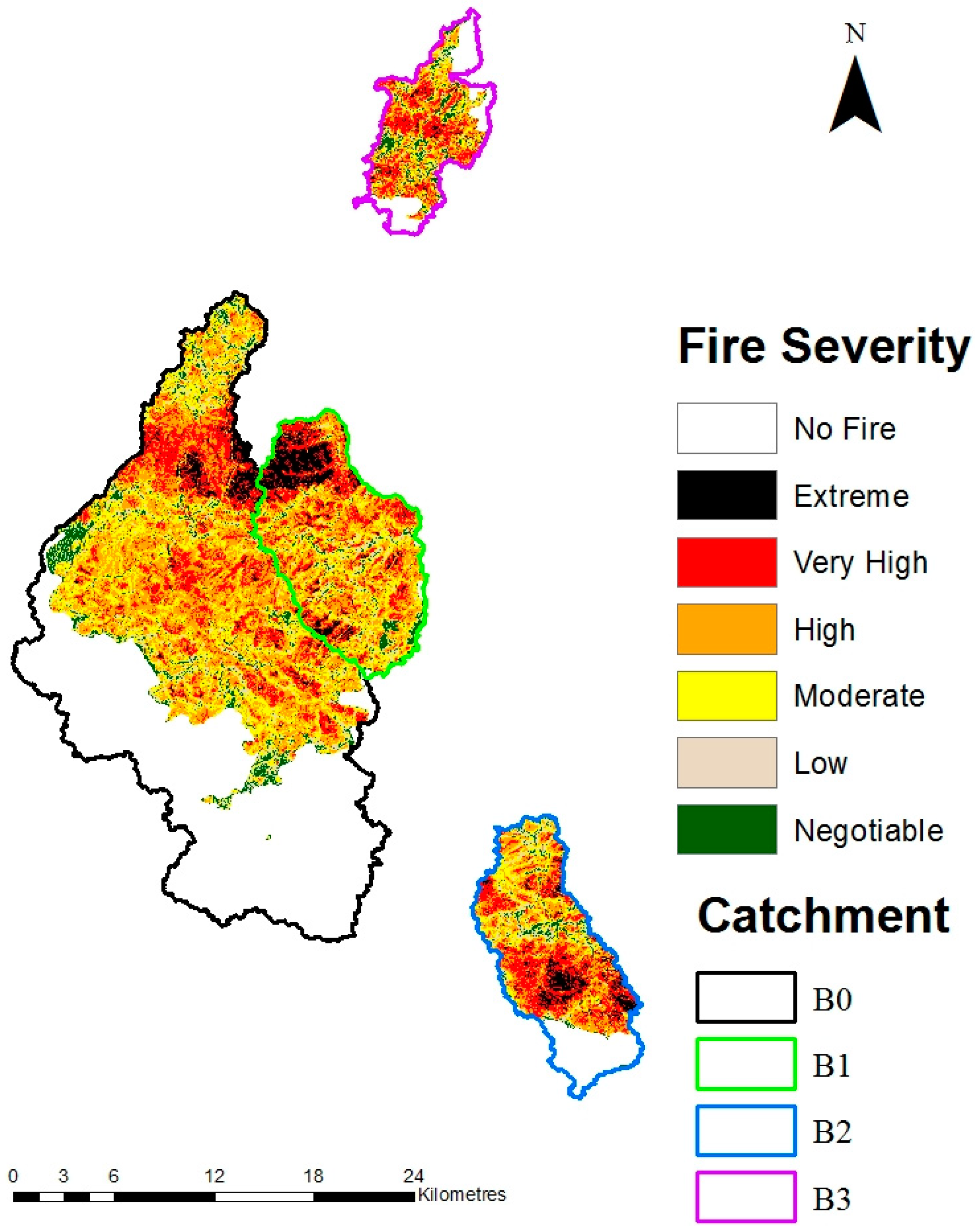
In this study, the three catchments not burnt during this wildfire were used as control catchments (C1, C2 and C3) to interpret the change detection results rather than being strict experimental controls. The four other catchments were heavily impacted by the wildfire of 2001 [34], especially catchment B1. The wildfire severity map derived from differenced Normalized Difference Vegetation Index (dNDVI) was extracted from Heath, et al. [35] based on the satellite interpretation of the wildfire behavior in the burnt catchments.

The fire severity map is showed in Figure 2. Catchment B1 was intensely affected by extreme wildfire, as shown in Table 2, and 100% of the catchment was burnt in this wildfire with the most intense wildfire occurring next to the monitoring station. Similar to B1, catchment B0 was significantly affected by extreme wildfire near the monitoring station. However, compared to B1, the percentage of area burnt in B0 catchment (57% burnt), is smaller than B2 (83% burnt), which also experienced less severe wildfire around the monitoring station compared to the other burnt parts of the catchment. The wildfire severity of catchment B3 (79% burnt), was more evenly distributed.

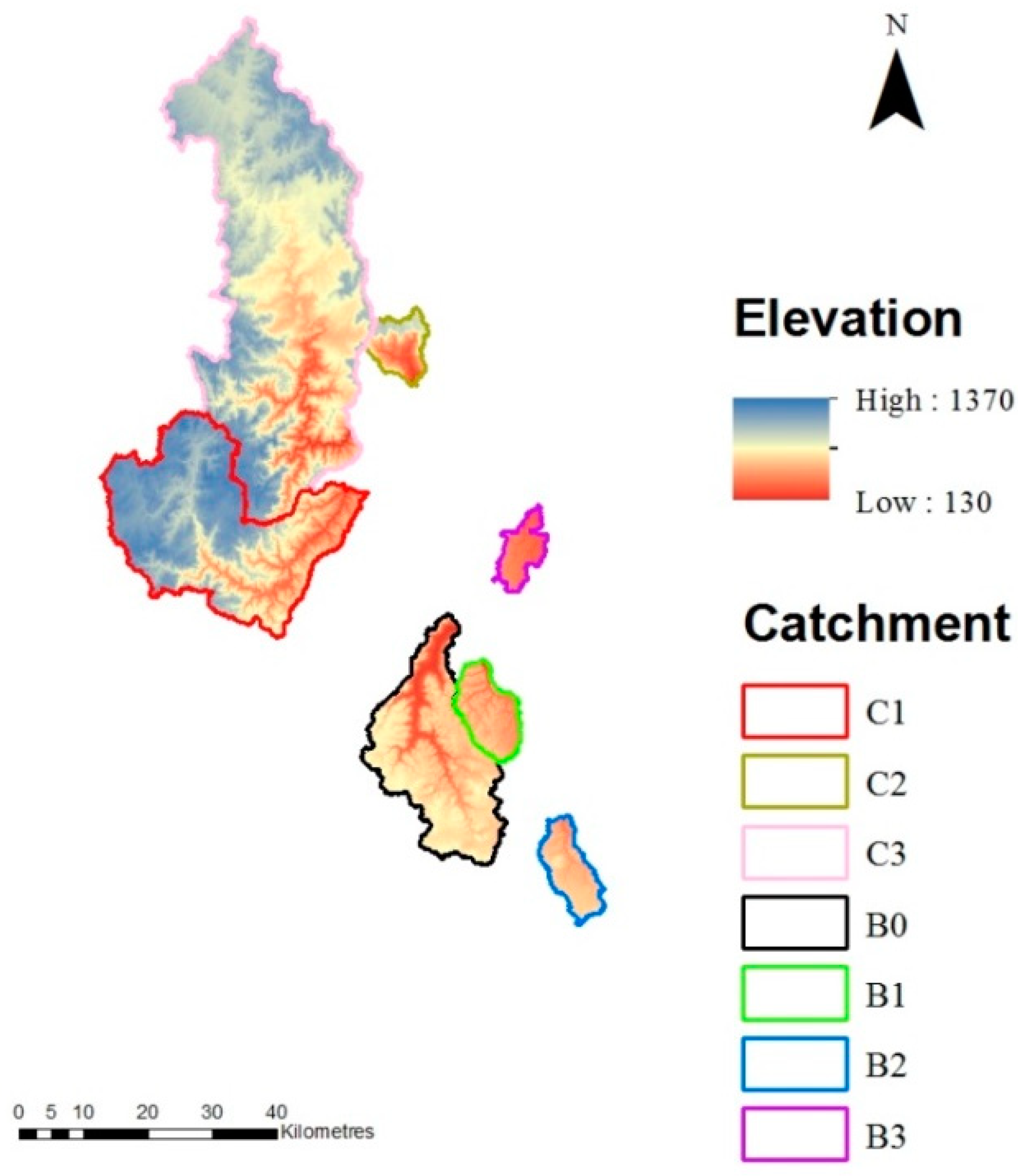
2.3. Catchment Terrain

Figure 3 presents elevation maps of the studied catchments. It shows the differences in elevation and terrain shape between the catchments. Catchment B0 has an elevation range from 105 m to 867 m, with a median slope of 8%. Catchment B1 has an elevation range from 175 m to 632 m, median slope 10%. Compared to these two catchments, catchment B3 and B2 are relatively flat. Catchment B3 has a median slope 3%, elevation ranges from 205 to 519. B2 has a minimum elevation of 328 m, maximum elevation of 777 m, median slope 4%.

2.4. Change Detection Method

In order to assess the medium term effect of wildfire on WQ, a linear mixed model (LMM) was used, with the focus being on modeling TSS, TN, and TP concentrations. The use of this LMM allows for an auto-correlation in the residuals to be modeled [33]. This is crucial, as the WQ samples have been collected systematically, so we cannot assume we have independent observations which would allow us to use least-squares regression [23]. The impact of this incorrect assumption would be biased standard errors, which has follow on effects on variable selection and hypothesis testing [33].

In this work we used a similar approach to Lessels and Bishop [33], who used flow and derivatives of flow to model WQ. The LMMs were fitted using the geoR package [36] in R [37]. To detect change due to the wildfire, a wildfire dummy variable (0 for pre-wildfire period, 1 for post-wildfire period) was created, and used as a predictor in all models irrespective of whether the catchment was burnt or unburnt. Our assumption is that: In the burnt catchments, the presence of the wildfire dummy variable in the final model indicates that there was an impact from the wildfire. The value of the coefficient associated with the wildfire dummy variable indicates the mean change in WQ between pre- and post-wildfire periods, assuming all of the other predictors are held to be constant. The interpretation of this has to be considered in the context of the unburnt catchments, which in an idealized situation would have a non-significant wildfire dummy variable, and therefore the coefficient would equal 0. This approach is analogous to an analysis of covariance (ANCOVA), except that here we use a more complex model to account for differences in flow and flow-related variables between the pre- and post-wildfire period, which are also related to WQ.

In addition to the wildfire dummy variable, the predictors we considered were event direction, event distance, discount flow (DF), and flow. The event distance is the time since the last event flow. An extended dry period will cause a buildup of easily erodible material in the catchment, which will cause higher concentrations (in terms of sediments and nutrients) during the first flow, and generally in the rising limb [38].

The event direction specifies whether the stream is in base flow conditions, the rising limb, or the falling limb of an event. The discount factor (DF) value, introduced by Wang, Kuhnert and Henderson [38], represents a weighted average of past flow that provides a measure of antecedent conditions. If the sequence $\widehat{q}$ up to time j, is ${({\widehat{q}}_m)}_{1 \le m \le j}$, then the DF value with discount factor d is defined as;

$$\mathrm{DF}\left(d\right)= \frac{{\sum }_{i-1}^j{d}^{j+1-i}{\widehat{q}}_j}{{\sum }_{i-1}^j{d}^{j+1-i}}$$

(1)

In summary, a weight, d, is given to historical observations to calculate a temporally weighted average of past flow. This weight diminishes exponentially with time at a rate that varies with the DF value. In general, a smaller DF value indicates that recent flows have more weighting, while a large DF value indicates the DF flow represents longer term flow conditions [38]. For the LMM, five levels of DF (0.50, 0.75, 0.9, 0.95 and 0.99) were considered as candidate predictor variables. The predictors were selected using backward elimination based on Wald tests using a p-value of 0.05 as the criteria for keeping predictors in the model.

After the model is predicted, the partial regression coefficient of the “wildfire” dummy variable was back-transformed to assess the impact of any wildfire in terms of the proportional increase or decrease in its effect on WQ on the original scale.

2.5. Assessment of Model Quality

Leave-one-out cross-validation was used to assess the model quality of the LMM. Measures of model quality were assessed by the mean and median standardized-squared prediction error (SSPE), mean error (ME), root-mean-square error (RMSE) and Lin’s Concordance Correlation Coefficient (Lin’s CCC). The SSPE for time, i, is

$$\mathrm{SSPE}\left(i\right)= \frac{{\{z\left(i\right)-\widehat{Z}\left(i\right)\}}^2}{{\sigma }_i^2}$$

(2)

where z is the observed value, $\widehat{Z}$ is the predicted value, and ${\sigma }_i^2$ is the prediction variance. A mean SSPE value close to 1 indicates that model estimates of uncertainty (the prediction variances) match the prediction errors, meaning that this model correctly represents the variation in WQ [23]. This is crucial, as the variance estimates associated with the partial regression coefficients are used to perform variable selection, and ultimately assess the change in WQ attributable to wildfire.

Root-mean-square error (RMSE) is the standard deviation of the residuals, and is a measure of the accuracy of the model. As the predictions get better, the RMSE becomes closer to 0.

The mean error is a measure of the bias of the model (3);

$$\mathrm{ME}=\frac{1}{n}{\sum }_{i=1}^{n}z\left(i\right)-\widehat{Z}\left(i\right).$$

(3)

It measures the average tendency of the predicted values to be larger or smaller than the observed values. The optimum value is 0.

Lin’s CCC (ρ_c) is a measure of how far pairs of observed and predicted values deviate from the line of perfect concordance, that is the 45° line of a scatter plot of observed versus predicted. It is scale-independent, and allows comparisons between properties with different magnitudes or units. The perfect value of Lin’s CCC is 1. When the two variables compared have a length of N, ρ_c is calculated as shown below (4);

$${\rho }_c=\frac{2s_{xy}}{s_x^2+s_y^2+{\left(\overline{x}-\overline{y}\right)}^2}$$

(4)

where $\overline{x}$ and $\overline{y}$ are the corresponding mean, $s_x^2$ and $s_y^2$ are variance, $s_{xy}$ is the covariance.

The flow and WQ data were log transformed to meet the assumption of normality for the LMM.

3. Results

3.1. Exploratory Data Analysis

A summary of the available water quality and quantity data is shown in

Table 3. Summary of flow and WQ data.

		Flow (ML/day)			TSS (mg/L)			TN (mg/L)			TP (mg/L)			Available Data
Catchment	Pre/Post-wildfire	Min	Max	Median	Min	Max	Median	Min	Max	Median	Min	Max	Median
C1	pre	0.88	65,000	181.51	0.5	3829	1.00	0.03	7.52	0.20	0.001	2.42	0.01	244
	post	0.23	16,673.89	908.45	0.5	532	4.00	0.005	2.25	0.31	0.003	0.34	0.02	536 *
C2	pre	5.66	6238.66	31.51	0.5	1316	3.00	0.2	15.8	1.13	0.001	1.5	0.16	220
	post	1.736	2202.96	87.48	0.5	536	6.00	0.005	2.08	0.36	0.002	0.39	0.01	284
C3	pre	11.11	101,778.8	191.10	0.5	2807	1.00	0.06	7.84	0.18	0.001	0.92	0.01	213
	post	3.28	8879.39	646.18	0.5	2149	5.00	0.05	13.2	0.30	0.002	1.92	0.01	331
B0	pre	0.54	2.39	0.62	0.5	15110	1.00	0.05	6.3	0.32	0.001	0.53	0.02	288
	post	0.53	0.99	0.56	0.5	1998	7.00	0.17	11.8	0.42	0.003	2.3	0.02	126
B1	pre	1.57	6828.59	6.77	0.5	97	1.00	0.005	9.4	0.10	0.001	0.26	0.004	218
	post	0.34	1126.86	5.48	0.5	3950	1.00	0.05	21.2	0.20	0.003	2.45	0.005	69 *
B2	pre	3.43	7491.3	21.80	1	149	1.00	0.03	0.79	0.16	0.001	0.17	0.009	157
	post	1.54	4067	55.77	0.5	35	1.25	0.005	0.95	0.17	0.001	0.06	0.008	381
B3	pre	0	14,299.22	9.565	0.5	803	4.0	0.05	6.8	0.42	0.001	0.73	0.01	233
	post	0	1184.46	32.29	0.5	496	7.0	0.005	2.65	0.44	0.003	0.5	0.02	351

*: Outliers compared to other catchments. Abbreviations: C = Control; B = Burnt; TSS = Total Suspended Sediment; TN = Total nitrate; TP = Total phosphate.

. The number of observations for WQ data is limited to around one per month; therefore, 200–300 observations are available for each catchment during both the pre-wildfire and post-wildfire period. Some big exceptions are C1, which had 500+ observations during the post-wildfire period and B1, which only had 69 observations collected in the post-wildfire period. For catchment B1, because most available data were collected before 2007, this might have resulted in a higher maximum and mean TSS value in this catchment because the catchment has had less time to recover during the post-wildfire period.

During 2001 to 2009, in the post-wildfire period, the studied catchments were affected by the millennium drought [39], especially during the first five years post-wildfire. The millennium drought was described as the worst drought on record for southeastern Australia: The Commonwealth Science and Industrial Research Organization (CSIRO) [40] found the lowest average precipitation since 1900 during this drought period. The millennium Drought is the longest uninterrupted series of years with below median rainfall in southeastern Australia since 1900 [39].

Table 4. Annual rainfall during pre-wildfire, 1–5 years post-wildfire and 6–10 years post-wildfire for all catchments (ML/day).

Catchment	Pre-Wildfire	1–5 years Post-Wildfire	6–10 years Post-Wildfire
C1	912.79	796.50	1111.44
C2	1214.06	1080.18	1556.01
C3	851.94	757.99	1091.89
B0	903.51	697.83	914.69
B1	869.25	671.38	880.01
B2	1246.38	962.65	1261.80
B3	670.72	592.18	849.14

presented the average annual rainfall estimated for each catchment using Thiessen polygons with data obtained from nearby Bureau of Meteorology weather stations. As summarized in Table 4, all catchments experienced a rainfall decrease during the first five years post-wildfire period. The decreases in catchment B0, B1, and B2 are most severe.

As a result, all the catchments showed a lower maximum flow value in the post-wildfire period compared to the pre-wildfire period (Table 3). A lower TSS maximum value is also observed in most catchments except catchment B1. Catchment B1 had a larger maximum TSS concentration during the post-wildfire period. This significant difference might be a result of the wildfire effect. In contrast to the maximum value, a higher post-wildfire median flow value is observed in most catchments except B0 and B1. A higher post-wildfire median TSS concentration is observed in all catchments, as compared to the pre-wildfire period. A higher post-wildfire maximum value of TN is observed in C3, B0, B1, and B2, as compared to the pre-wildfire period. In terms of TP a higher post-wildfire value is observed in C3, B0, and B1. Most catchments observed a higher median TN and TP value during the post-wildfire period, except catchment C2.

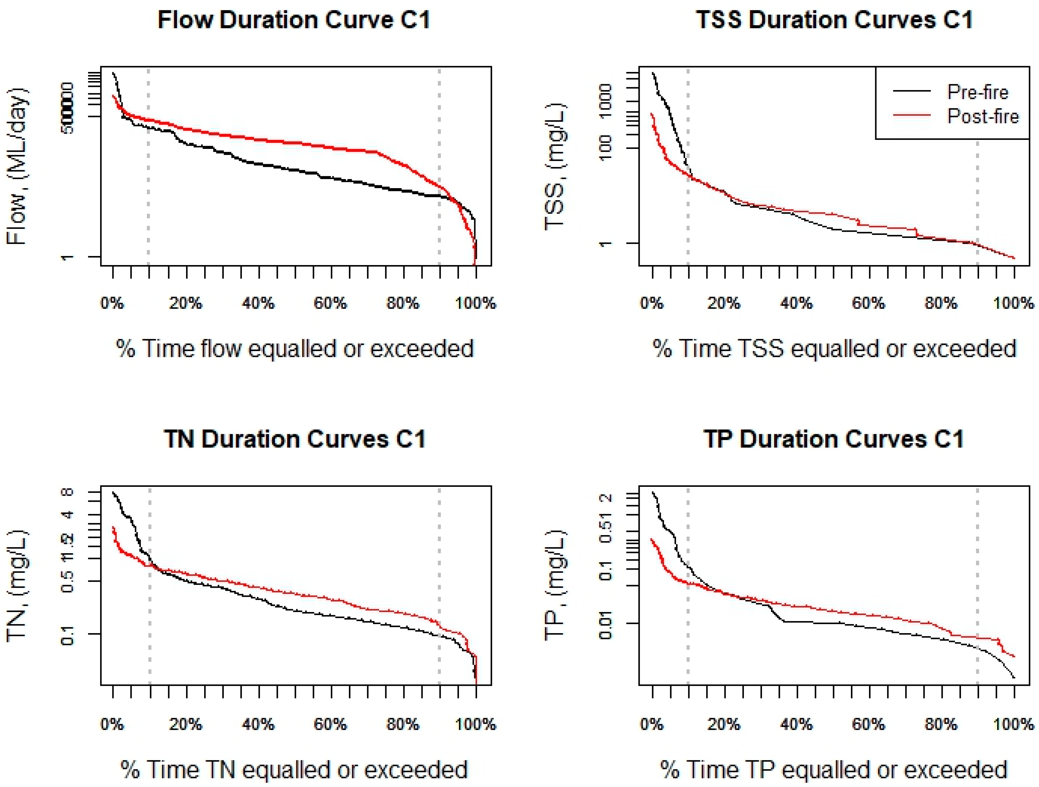
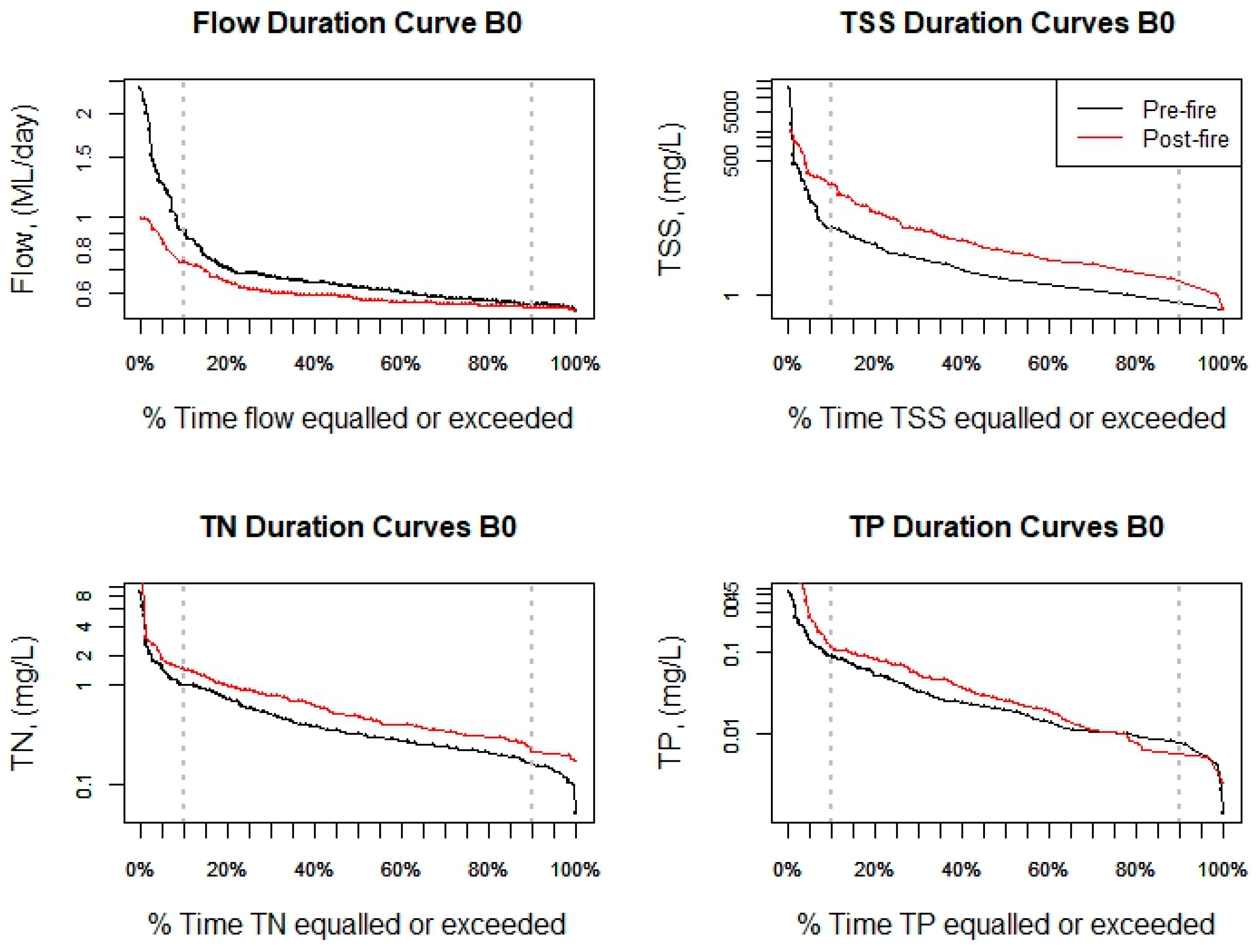
The change in the maximum values might indicate a change in flow duration curve; this might result in a WQ concentration change. An example of duration curves pre- and post-wildfire is shown for catchments C1 and B0 in Figure 4 and Figure 5. During the post-wildfire period, the catchments experienced a change in the distribution of flow and WQ as represented by the duration curves. The flow duration curve for catchment C1 shows that compared to the pre-wildfire period, the post-wildfire period showed a decrease in flow for the top decile, and an increase in the middle decile of the graph. This explained the increase in median value of the data as summarized in Table 3. The bottom decile of the flow duration curve showed a similar pattern to the pre-wildfire period. A similar pattern was also evident in the WQ duration curves for the control catchments; a decrease in top and bottom deciles of the curve, and an increase in the middle decile. Catchment B0 experienced a greater rainfall decrease, which resulted in a more obvious decrease in both peak flow and base flow in the flow duration curves as shown in Figure 5. Opposite to the control catchment, a decrease in flow in the middle decile of the graph is observed. However, an upshift of the WQ duration curves was observed in all WQ duration curves for catchment B0. The change in the maximum and median flow value and the change in duration curves shows the WQ change might be effected by the change of flow, and it is important to account for flow when detecting the effect of wildfire on WQ.

3.2. Linear Mixed Modelling

All models showed a mean SSPE close to 1 and a negligible bias (

Table 5. Model performance.

	TSS				TN				TP
Catchment	Mean SSPE	ME	RMSE	Lin’s CCC	Mean SSPE	ME	RMSE	Lin’s CCC	Mean SSPE	ME	RMSE	Lin’s CCC
C1	0.96	−0.03	0.94	0.79	0.96	−0.03	0.43	0.85	0.96	−0.04	0.61	0.83
C2	1.02	0.00	1.12	0.76	0.97	0.01	0.59	0.81	1.03	0.00	0.87	0.84
C3	0.99	−0.03	0.97	0.76	1.03	−0.02	0.55	0.78	0.99	−0.01	0.69	0.73
B0	0.98	−0.01	1.04	0.81	0.96	−0.01	0.51	0.73	0.90	−0.01	0.69	0.78
B1	0.98	−0.01	0.89	0.74	0.97	−0.01	0.87	0.71	0.97	0.00	0.84	0.70
B2	1.00	0.01	0.73	0.65	1.05	−0.01	0.48	0.74	0.98	0.00	0.54	0.70
B3	1.00	−0.03	0.93	0.77	0.96	−0.03	0.43	0.77	0.94	−0.01	0.53	0.81

Abbreviations: C = Control; B = Burnt; TSS = Total Suspended Sediment; TN = Total Nitrate; TP = Total Phosphate.

), indicating a good model performance. This means that we can be confident that the variances are unbiased, and our variable selection is valid. The model performance was also quite consistent between catchments and WQ variables, as evidenced by the Lin’s CCC values ranging from 0.65–0.85 for all models. Each catchment had a different combination of predictors for predicting TSS, TN and TP (

Table 6. Selected predictors for model predicting total suspended solids.

TSS	Log Flow	Event Direction	Event Distance	DF50	DF75	DF90	DF95	DF99	Wildfire
C1
C2
C3
B0
B1
B2
B3

Abbreviations: C = Control; B = Burnt; TSS = Total Suspended Sediment; DF = Discount Flow.

,

Table 7. Selected predictors for model predicting total nitrogen.

TN	Log Flow	Event Direction	Event Distance	DF50	DF75	DF90	DF95	DF99	Wildfire
C1
C2
C3
B0
B1
B2
B3

Abbreviations: C = Control; B = Burnt; TN = Total Nitrate; DF = Discount Flow.

and

Table 8. Selected predictors for model predicting total phosphorus.

TP	Log Flow	Event Direction	Event Distance	DF50	DF75	DF90	DF95	DF99	Wildfire
C1
C2
C3
B0
B1
B2
B3

Abbreviations: C = Control; B = Burnt; TP = Total Phosphate; DF = Discount Flow.

). All models found flow to be a significant predictor for predicting WQ. Furthermore, models for predicting TSS generally found event direction to be a useful predictor. Much less (two models in TN and three models in TP prediction) catchments found this to be significant in models predicting TN and TP. One possible reason is that TN and TP includes soluble N and P, which are not as tightly coupled to runoff and erosion events. The models for C2 and B2 as shown in Table 6 have indicated both event direction and event distance as a predictor for TSS, while other models included either event direction or event distance. C3, B0, B1 and B3 models indicated wildfire as a predictor for TSS. For total nitrogen, model C2, B0, B1, B2 and B3 predicted a wildfire effect. For total phosphorus, catchments C2, B1, and B2 indicated that wildfire is a significant predictor.

The back-transformed model coefficients are showed in

Table 9. Back-transformed model coefficients for wildfire dummy variable, indicating effects of wildfire on WQ.

Catchment	TSS	TN	TP
C1	X	X	X
C2	X	0.37	0.1
C3	1.46	X	X
B0	3.32	1.35	X
B1	1.84	2.88	2.45
B2	X	0.7	1.13
B3	1.32	X	X
Average for control *,1	1.23	1	1
Average for burned *	1.87	1.48	1.40
Net change (burnt-control)	0.64	0.48	0.40

* for calculating the Average, when the effect of wildfire was not significant a value of 1 was used. ¹: catchment C2 was not used to calculate the mean due the STP upgrading during the post-wildfire period.

. Among the three control catchments, catchment C3 showed an increased in TSS during the post-wildfire period. The lower amount of available data for the C3 catchment may have contributed to this result (Table 3). This is because pre-wildfire there were no auto-samplers, so the number of event samples would have been small, resulting in an under-estimation of the mean WQ values in the pre-wildfire period. This would not be case in the other catchments, since with more samples, the entire range of flow conditions is represented as found by the work of [27] in the same catchments. Additionally, catchment C2 showed a decrease in both TN and TP levels (Table 9). Catchment C2 is located downstream from a sewage treatment plant (STP) which was upgraded around the time of the wildfire, so that this upgrade would have improved the WQ in catchment C2 and effected our results. Thus, the results from C2 were removed before calculating the mean effect for Table 9. However, the TN and TP decreases observed in the modeling process gives confidence in our approach, and shows its applicability to change detection studies in general. All burnt catchments except B2 showed a wildfire effect on TSS. Catchment B1 showed the largest TSS increase during the post-wildfire period. The wildfire effect on TSS in catchment B2 was not observed. Table 9 also presents the average of the back transformed regression coefficient for the control and burnt catchments. The burnt catchments show a 40–87% increase in TN, TP and TSS for the post-wildfire period, whereas the control catchments observed a 23% increase in TSS, and no change for either TN or TP.

4. Discussion and Conclusions

An increase in TSS value after a wildfire is a main observation in many studies [8]. It is also observed in this study on a decade scale. In terms of individual catchments there were fluctuations in the impacts of the wildfire. On average, in the 10 year post-wildfire period, catchment B0 showed the highest increase in TSS (3.32 fold more than pre-wildfire), followed by B1 (1.84 fold increase over pre-wildfire) and catchment B3 showed a relatively lower effect (1.32 fold increase over pre-wildfire). Catchment B2 did not show a statistically significant TSS concentration change. This can be caused by several reasons: Firstly, catchment B2 had a small amount of pre-wildfire data relative to the post-wildfire data. Therefore, the standard errors associated with the dummy wildfire variable would be large, making it less likely to find a significant difference. Secondly, this result could also be caused by the lower wildfire severity in the catchment. Finally, the monitoring station is located further away from most severely burnt parts of the catchment (Figure 1 and Figure 2), which possibly make changes in WQ, being modeled less sensitive to wildfire effects.

An increase in TSS value after wildfire is a main observation in many past studies [8]. However, the study results varies: Malmon, Reneau, Katzman, Lavine and Lyman [29] observed a 33-fold increase in TSS in their study on the water quality change three months post-wildfire; Sheridan, et al. [41] observed a 32-fold increase in TSS after one year of the wildfire. Conversely, some catchments were less effected by wildfire, for example, Gallaher, et al. [42] observed a 1.76-fold increase in TSS level five months post-wildfire. Past studies also showed that the recovery time of a catchment varies between studies based on different burnt severity and other catchment conditions, for example at one extreme, Hicke, et al. [43] found that catchment recovery to pre-wildfire conditions took three months post-wildfire. On the other side, another study indicates complete catchment flow condition recovery may take as long as 150 years [9]. Compared to past studies focused on the WQ in the first three years post-wildfire, our study tested the 10 years average effect. As a result, our predictions of the effect of wildfire on TSS in the medium term are considerably smaller than studies using short-term post-wildfire data. Compare to Townsend and Douglas’ study [12] on the 10th year post-wildfire WQ, their study observed no obvious WQ change, while our study on 10 years average WQ change observed a more obvious change. This can be explained by a few reasons: Firstly, the fire severity in their catchments was low: Their catchment was burnt in May, which is a wet season for the catchment. Secondly, only three years pre-wildfire data were used in their study, which may not fully reflect the pre-wildfire conditions of the catchment. Thirdly, their study tested the WQ collected on the 10th year after wildfire, and this will make the WQ change observation less intense than our test on the 10 year average of post-wildfire period, which includes the early years post-wildfire when the change would be larger.

Relative to TSS, the impact of wildfire on TN and TP is less pronounced [19,44,45,46]. Past studies have shown small declines to minor increases of TN and TP (0.2, 2 fold respectively) and also large increases (between 20 to 432 fold) [12,28,47]. Our LMM results showed in a medium term a 2.88 fold increase in TN for the most severely burnt catchment, catchment B1, and 2.45 fold increase in TP. Catchment B1 has a shorter record of post-wildfire available data (up to six years post-wildfire only), which might be the reason for the large change in WQ. Additionally, the higher averaged change in six year averaged WQ concentration change compared to longer (10 years) average change, demonstrated a sign of catchment recovery as WQ concentrations recover towards the pre-wildfire level. This also indicates that this catchment was still significantly impacted by the wildfire up to six years post-wildfire. This is far longer than several other studies which found that TN and TP concentration returns to the pre-wildfire level 1–2 years post-wildfire, and TN may decrease in the medium term [8,48,49]. A decrease in TN was also reported by our catchment B2. The increases in TN and TP concentration during the post-wildfire period may result from the remobilization of sediment store in colluvial deposits, channels and floodplain, as well as from atmospheric and runoff inputs of ash [8]. The nutrient losses from unburnt forested catchments are usually low [14]. In contrast, wildfire volatilizes nutrients from vegetation and soil. These nutrients are either released into atmosphere or remain in the ash deposited on the soil surface [43]. Nutrients that remain in the surface ash layer may be transported into streams during run-off and erosion events [14]. The amount of N and P lost from soil is directly related to the amount of organic matter destroyed during a wildfire [50]. One observation from our study is post-wildfire TN and TP is sensitive to flow, but less sensitive to event type (event duration and event antecedent condition) than TSS. This might indicate that the post-wildfire TN and TP are less related to catchment erosion and runoff from the surface layer during rainfall events, because rather a large proportion of TN and TP is transferred into streams from infiltration.

One major limitation of this study is ignoring the effect of wildfire on different parts of the hydrograph, for example base flow vs. event flow. Further research should focus on examining the effect of wildfire on event WQ, and also distinguish between short term (0–2 years post-wildfire) and medium term (2+ years post-wildfire) impacts on WQ. Additionally, in this study, only empirical models has been reviewed and used for detecting change. Empirical models, compared to any physical-based distributed model, requires less data and processing time.

However, the empirical methods used here lack the ability to incorporate within-catchment spatial variability, e.g., soil, topography, into the modeling process [27]. Future research should consider the use of a distributed model for analysis of fire effects on water quality so the topography differences can be included in the modeling/analysis process.

In this study we have used LMM to compare 10 years pre- and post-wildfire TSS, TN and TP change after a wildfire in Australia. On average, there is a 64% TSS concentration increase, a 48% TN concentration increase and 40% TP increase during the 10 years post-wildfire period. This study has shown that wildfires can have a significant effect on water quality over long-term, decadal timescales. For efficient catchment monitoring and management, a long term (10+ years) water quality monitoring is essential.

References

- Shakesby, R.A.; Doerr, S.H. Wildfire as a hydrological and geomorphological agent. Earth-Sci. Rev. 2006, 74, 269–307. [Google Scholar] [CrossRef]
- Ice, G.G.; Neary, D.G.; Adams, P.W. Effects of wildfire on soils and watershed processes. J. For. 2004, 102, 16–20. [Google Scholar]
- Crouch, R.L.; Timmenga, H.J.; Barber, T.R.; Fuchsman, P.C. Post-fire surface water quality: Comparison of fire retardant versus wildfire-related effects. Chemosphere 2006, 62, 874–889. [Google Scholar] [CrossRef] [PubMed]
- Lane, P.N.J.; Feikema, P.M.; Sherwin, C.B.; Peel, M.C.; Freebairn, A.C. Modelling the long term water yield impact of wildfire and other forest disturbance in eucalypt forests. Environ. Model. Softw. 2010, 25, 467–478. [Google Scholar] [CrossRef]
- Neary, D.G.; Ice, G.G.; Jackson, C.R. Linkages between forest soils and water quality and quantity. For. Ecol. Manag. 2009, 258, 2269–2281. [Google Scholar] [CrossRef]
- Lucas, C. Bushfire Weather in Southeast Australia: Recent Trends and Projected Climate Change Impacts; Bushfire Cooperative Research Centre: Melbourne, Australia, 2007. [Google Scholar]
- Lane, P.N.J.; Sheridan, G.J.; Noske, P.J. Changes in sediment loads and discharge from small mountain catchments following wildfire in South Eastern Australia. J. Hydrol. 2006, 331, 495–510. [Google Scholar] [CrossRef]
- Smith, H.G.; Sheridan, G.J.; Lane, P.N.J.; Nyman, P.; Haydon, S. Wildfire effects on water quality in forest catchments: A review with implications for water supply. J. Hydrol. 2011, 396, 170–192. [Google Scholar] [CrossRef]
- Kuczera, G.; Parent, E. Monte carlo assessment of parameter uncertainty in conceptual catchment models: The metropolis algorithm. J. Hydrol. 1998, 211, 69–85. [Google Scholar] [CrossRef]
- Drewry, J.J.; Newham, L.T.H.; Greene, R.S.B.; Jakeman, A.J.; Croke, B.F.W. A review of nitrogen and phosphorus export to waterways: Context for catchment modelling. Mar. Freshw. Res. 2006, 57, 757–774. [Google Scholar] [CrossRef]
- Wood, P.J.; Armitage, P.D. Biological effects of fine sediment in the lotic environment. Environ. Manag. 1997, 21, 203–217. [Google Scholar] [CrossRef]
- Townsend, S.A.; Douglas, M.M. The effect of a wildfire on stream water quality and catchment water yield in a tropical savanna excluded from fire for 10 years (Kakadu National Park, North Australia). Water Res. 2004, 38, 3051–3058. [Google Scholar] [CrossRef]
- Moody, J.A.; Martin, D.A. Post-fire, rainfall intensity–peak discharge relations for three mountainous watersheds in the western USA. Hydrol. Process. 2001, 15, 2981–2993. [Google Scholar] [CrossRef]
- Neary, D.G.; Ryan, K.C.; DeBano, L.F. Wildland Fire in Ecosystems: Effects of Fire on Soils and Water; U.S. Department of Agriculture, Forest Service: Ogden, UT, USA, 2005.
- Onda, Y.; Dietrich, W.E.; Booker, F. Evolution of overland flow after a severe forest fire, point reyes, California. Catena 2008, 72, 13–20. [Google Scholar] [CrossRef]
- Heath, J.T.; Chafer, C.J.; Bishop, T.F.; Van Ogtrop, F.F. Wildfire effects on soil carbon and water repellency under eucalyptus forest in eastern australia. Soil Res. 2015, 53, 13–23. [Google Scholar] [CrossRef]
- Johansen, M.P.; Hakonson, T.E.; Whicker, F.W.; Breshears, D.D. Pulsed redistribution of a contaminant following forest fire. J. Environ. Qual. 2003, 32, 2150–2157. [Google Scholar]
- Kuczera, G. Prediction of water yield reductions following a bushfire in ash-mixed species eucalypt forest. J. Hydrol. 1987, 94, 215–236. [Google Scholar] [CrossRef]
- Bladon, K.D.; Silins, U.; Wagner, M.J.; Stone, M.; Emelko, M.B.; Mendoza, C.A.; Devito, K.J.; Boon, S. Wildfire impacts on nitrogen concentration and production from headwater streams in southern alberta‘s rocky mountains. Can. J. For. Res. 2008, 38, 2359–2371. [Google Scholar] [CrossRef]
- Oliver, A.A.; Reuter, J.E.; Heyvaert, A.C.; Dahlgren, R.A. Water quality response to the angora fire, lake tahoe, California. Biogeochemistry 2012, 111, 361–376. [Google Scholar] [CrossRef]
- Bartley, R.; Speirs, W.J.; Ellis, T.W.; Waters, D.K. A review of sediment and nutrient concentration data from australia for use in catchment water quality models. Mar. Pollut. Bull. 2012, 65, 101–116. [Google Scholar] [CrossRef] [PubMed]
- Lessels, J.; Bishop, T. A simulation based approach to quantify the difference between event-based and routine water quality monitoring schemes. J. Hydrol. Reg. Stud. 2015, 4, 439–451. [Google Scholar] [CrossRef] [Green Version]
- Lark, R.M.; Cullis, B.R. Model-based analysis using reml for inference from systematically sampled data on soil. Eur. J. Soil Sci. 2004, 55, 799–813. [Google Scholar] [CrossRef]
- Salavati, B.; Oudin, L.; Furusho-Percot, C.; Ribstein, P. Modeling approaches to detect land-use changes: Urbanization analyzed on a set of 43 us catchments. J. Hydrol. 2016, 538, 138–151. [Google Scholar] [CrossRef]
- Ravichandran, S. Hydrological influences on the water quality trends in tamiraparani basin, South India. Environ. Monit. Assess. 2003, 87, 293–309. [Google Scholar] [CrossRef]
- Drewry, J.; Newham, L.; Croke, B. Suspended sediment, nitrogen and phosphorus concentrations and exports during storm-events to the Tuross Estuary, Australia. J. Environ. Manag. 2009, 90, 879–887. [Google Scholar] [CrossRef]
- Lessels, J.S.; Bishop, T.F. Using the precision of the mean to estimate suitable sample sizes for monitoring total phosphorus in australian catchments. Hydrol. Process. 2015, 29, 950–964. [Google Scholar] [CrossRef]
- Mast, M.A.; Clow, D.W. Effects of 2003 wildfires on stream chemistry in glacier national park, montana. Hydrol. Process. 2008, 22, 5013–5023. [Google Scholar] [CrossRef]
- Malmon, D.V.; Reneau, S.L.; Katzman, D.; Lavine, A.; Lyman, J. Suspended sediment transport in an ephemeral stream following wildfire. J. Geophys. Res. Earth Surf. 2007, 112. [Google Scholar] [CrossRef]
- Kunze, M.D.; Stednick, J.D. Streamflow and suspended sediment yield following the 2000 bobcat fire, colorado. Hydrol. Process. Int. J. 2006, 20, 1661–1681. [Google Scholar] [CrossRef]
- Hauer, F.R.; Spencer, C.N. Phosphorus and nitrogen dynamics in streams associated with wildfire: A study of immediate and longterm effects. Int. J. Wildland Fire 1998, 8, 183–198. [Google Scholar] [CrossRef]
- Winter, J.; Watts, M. Christmas fires 2001, commemorative edition. Bushfire Bull. 2002, 23, 1–160. [Google Scholar]
- Lessels, J.; Bishop, T. Estimating water quality using linear mixed models with stream discharge and turbidity. J. Hydrol. 2013, 498, 13–22. [Google Scholar] [CrossRef]
- Shakesby, R.A.; Wallbrink, P.J.; Doerr, S.H.; English, P.M.; Chafer, C.J.; Humphreys, G.S.; Blake, W.H.; Tomkins, K.M. Distinctiveness of wildfire effects on soil erosion in south-east australian eucalypt forests assessed in a global context. For. Ecol. Manag. 2007, 238, 347–364. [Google Scholar] [CrossRef]
- Heath, J.T.; Chafer, C.J.; van Ogtrop, F.F.; Bishop, T.F.A. Post-wildfire recovery of water yield in the sydney basin water supply catchments: An assessment of the 2001/2002 wildfires. J. Hydrol. 2014, 519 Pt B, 1428–1440. [Google Scholar] [CrossRef]
- Ribeiro, P.J., Jr.; Diggle, P.J. Geor: A package for geostatistical analysis. R News 2001, 1, 14–18. [Google Scholar]
- R Core Team. R: A Language and Environment for Statistical Computing. R Foundation for Statistical Computing; R Foundation for Statistical Computing: Vienna, Austria, 2015. [Google Scholar]
- Wang, Y.-G.; Kuhnert, P.; Henderson, B. Load estimation with uncertainties from opportunistic sampling data–a semiparametric approach. J. Hydrol. 2011, 396, 148–157. [Google Scholar] [CrossRef]
- van Dijk, A.I.; Beck, H.E.; Crosbie, R.S.; de Jeu, R.A.; Liu, Y.Y.; Podger, G.M.; Timbal, B.; Viney, N.R. The millennium drought in southeast australia (2001–2009): Natural and human causes and implications for water resources, ecosystems, economy, and society. Water Resour. Res. 2013, 49, 1040–1057. [Google Scholar] [CrossRef]
- South Eastern Australian Climate Initiative. Climate Variability and Change in South-Eastern Australia: A Synthesis of Findings from Phase 1 of the South Eastern Australian Climate Initiative (seaci); CSIRO Australia: Canberra, Australia, 2010.
- Sheridan, G.J.; Lane, P.N.; Noske, P.J. Quantification of hillslope runoff and erosion processes before and after wildfire in a wet eucalyptus forest. J. Hydrol. 2007, 343, 12–28. [Google Scholar] [CrossRef]
- Gallaher, B.; Koch, R.; Mullen, K. Quality of Storm Water Runoff at Los Alamos National Laboratory in 2000 with Emphasis on the Impact of the Cerro Grande Fire; Los Alamos National Laboratory LA-13926; Los Alamos National Laboratory: Los Alamos, NM, USA, 2002; p. 166.
- Hicke, J.A.; Allen, C.D.; Desai, A.R.; Dietze, M.C.; Hall, R.J.; Hogg, E.H.T.; Kashian, D.M.; Moore, D.; Raffa, K.F.; Sturrock, R.N. Effects of biotic disturbances on forest carbon cycling in the United States and canada. Glob. Chang. Biol. 2012, 18, 7–34. [Google Scholar] [CrossRef]
- Abramson, L. Post-Fire Sedimentation and Flood Risk Potential in the Mission Creek Watershed of Santa Barbara; University of California: Santa Barbara, CA, USA, 2009. [Google Scholar]
- Feikema, P.M.; Sheridan, G.J.; Argent, R.M.; Lane, P.N.J.; Grayson, R.B. Estimating catchment-scale impacts of wildfire on sediment and nutrient loads using the e2 catchment modelling framework. Environ. Model. Softw. 2011, 26, 913–928. [Google Scholar] [CrossRef]
- Lane, P.N.J.; Sheridan, G.J.; Noske, P.J.; Sherwin, C.B. Phosphorus and nitrogen exports from se Australian forests following wildfire. J. Hydrol. 2008, 361, 186–198. [Google Scholar] [CrossRef]
- Sheridan, G.; Lane, P.; Noske, P.; Feikema, P.; Sherwin, C.; Grayson, R. Impact of the 2003 Alpine Bushfires on Streamflow: Estimated Changes in Stream Exports of Sediment, Phosphorus and Nitrogen Following the 2003 Bushfires in Eastern Victoria; Murray-Darling Basin Commission: Canberra, Australia, 2007.
- Hopmans, P.; Bren, L.J. Long-term changes in water quality and solute exports in headwater streams of intensively managed radiata pine and natural eucalypt forest catchments in South-Eastern Australia. For. Ecol. Manag. 2007, 253, 244–261. [Google Scholar] [CrossRef]
- Porporato, A.; D’Odorico, P.; Laio, F.; Rodriguez-Iturbe, I. Hydrologic controls on soil carbon and nitrogen cycles. I. Modeling scheme. Adv. Water Resour. 2003, 26, 45–58. [Google Scholar] [CrossRef]
- Hart, S.C.; DeLuca, T.H.; Newman, G.S.; MacKenzie, M.D.; Boyle, S.I. Post-fire vegetative dynamics as drivers of microbial community structure and function in forest soils. For. Ecol. Manag. 2005, 220, 166–184. [Google Scholar] [CrossRef]
Figure 1.
Study area.
Figure 2.
Wildfire severity maps of burnt catchments. Abbreviations: B = Burnt (Source: [35]).
Figure 3.
Elevation maps of studied catchments. Abbreviations: C = Control; B = Burnt.
Figure 4.
Duration curves for catchment C1. Abbreviations: C = Control; Q = Flow; TSS = Total Suspended Sediment; TN = Total nitrate; TP = Total phosphate.
Figure 5.
Duration curves for catchment B0 Abbreviations: B = Burnt; Q = Flow; TSS = Total Suspended Sediment; TN = Total nitrate; TP = Total phosphate.