Assessment of the Role of Snowmelt in a Flood Event in a Gauged Catchment

 , , and
Abstract
:
1. Introduction
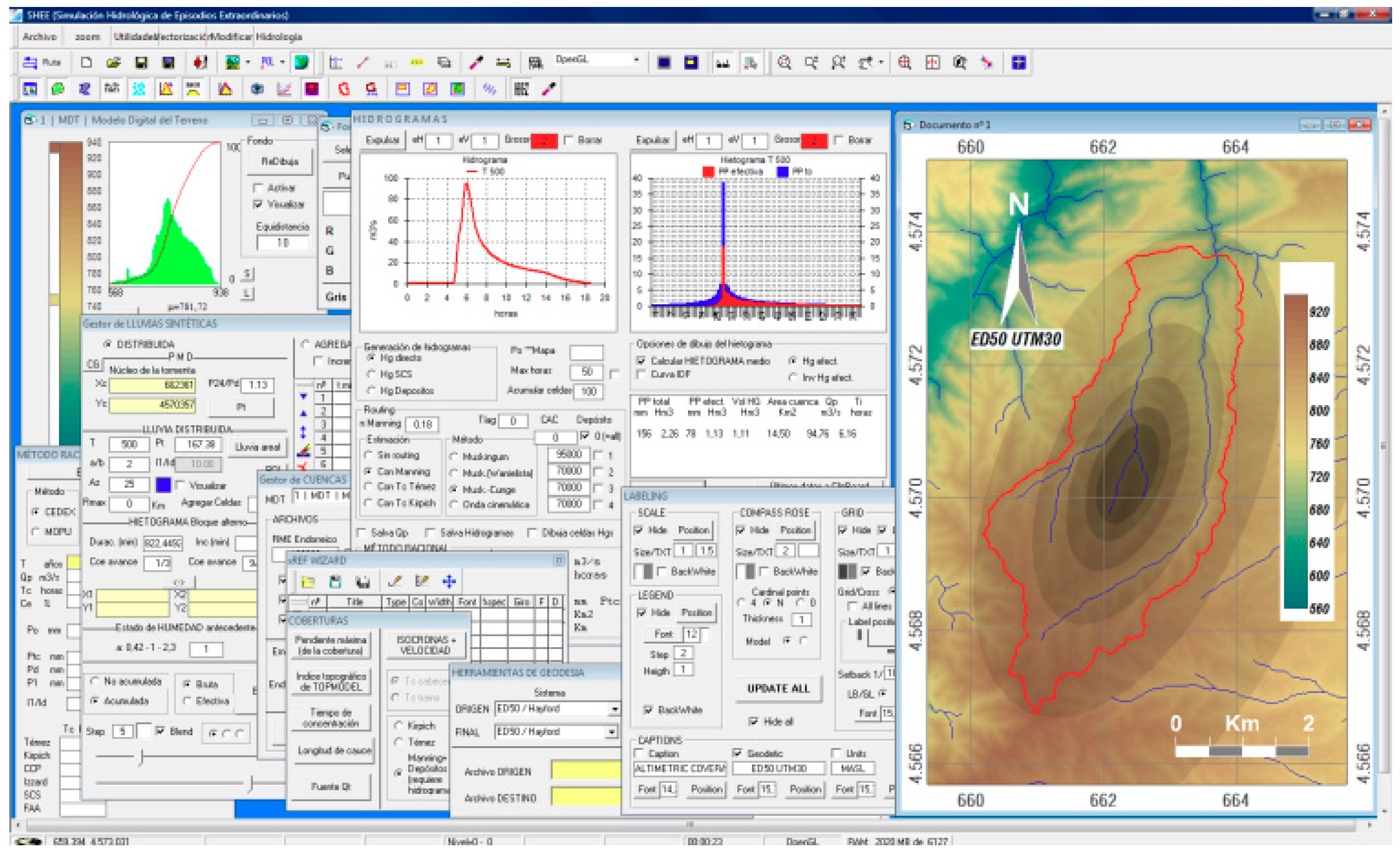
2. Methods
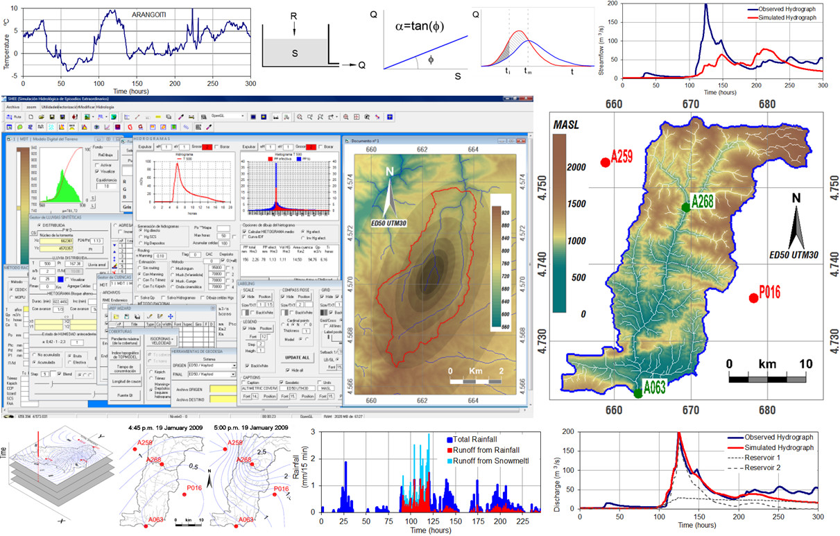
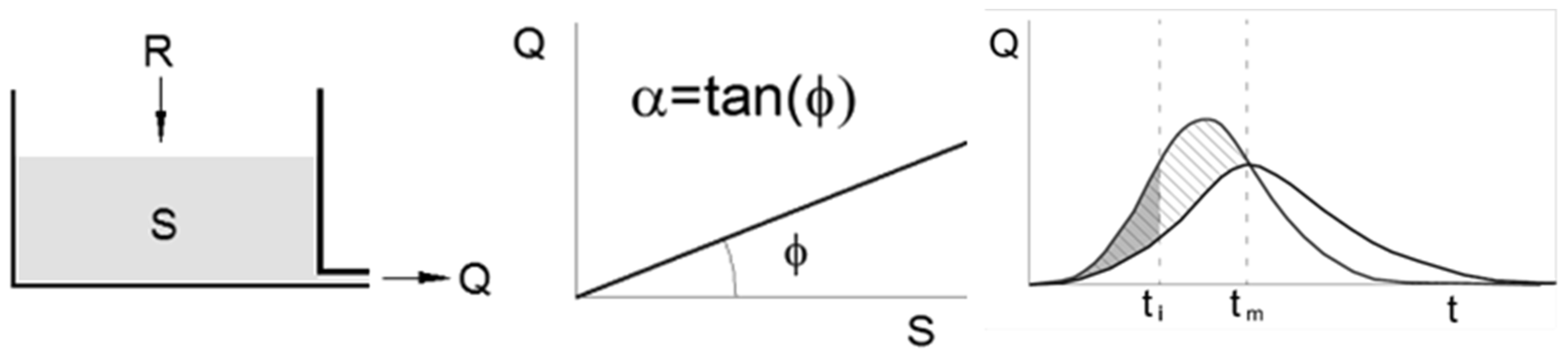
2.1. PLR Models: Characterization of a Single Linear Reservoir
2.2. PLR Models: Combination of Linear Reservoirs in Parallel Sets
2.3. PLR Models: Snowmelt
3. Data Sources
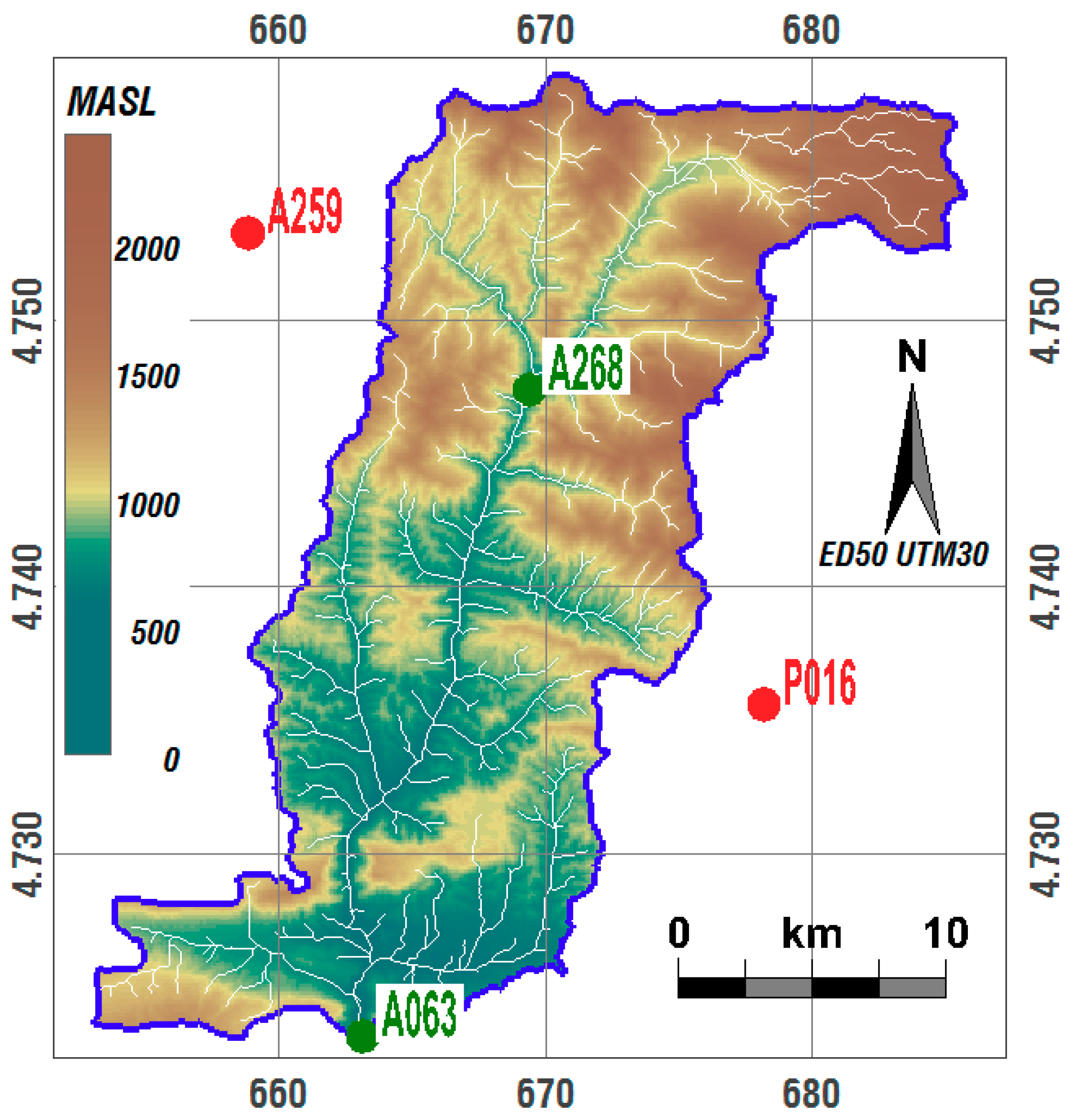
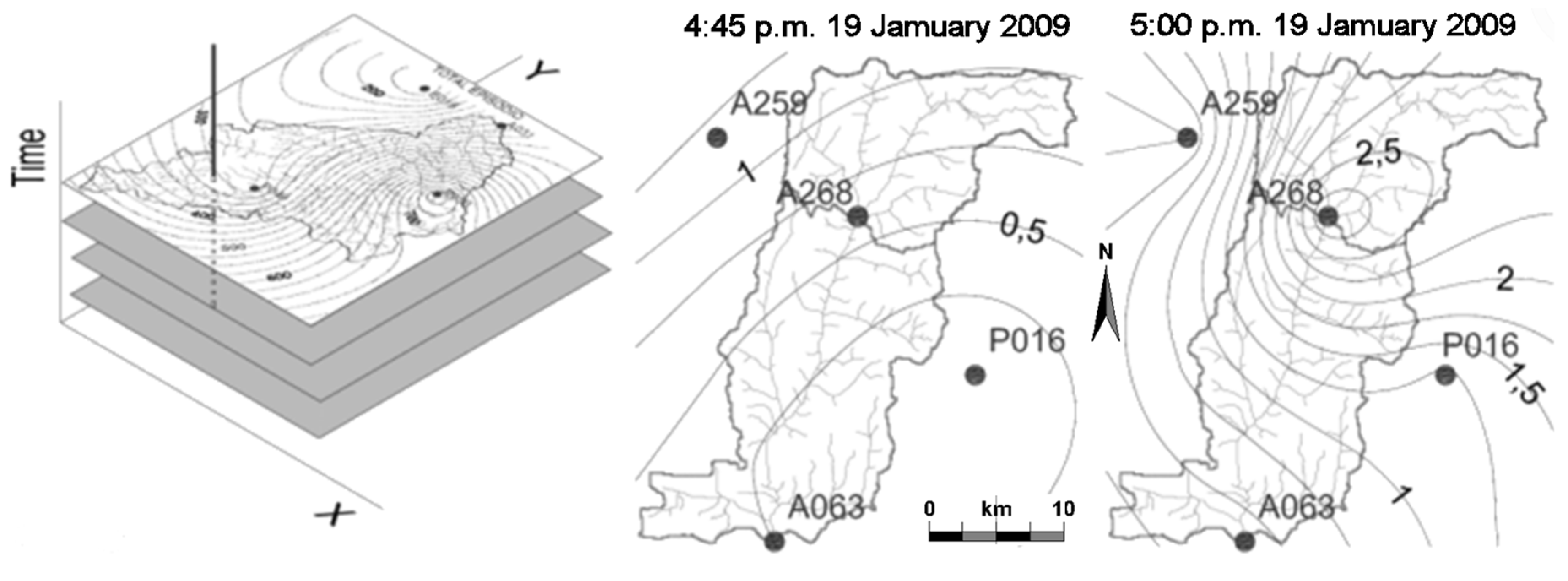
3.1. Characterization of the Basin
3.2. Melting Event Setting
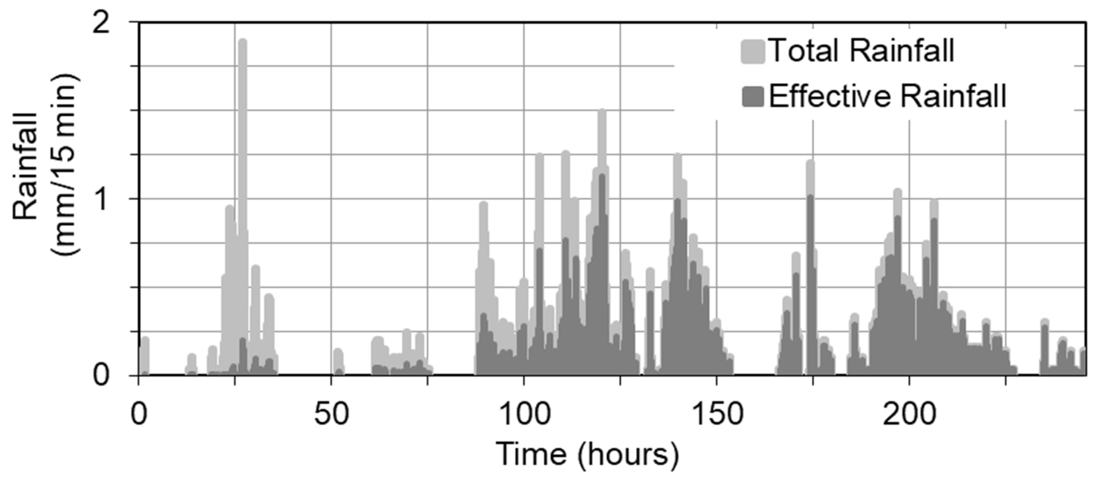
3.3. Rainfall Model
3.4. Reservoir Model
4. Results and Discussion
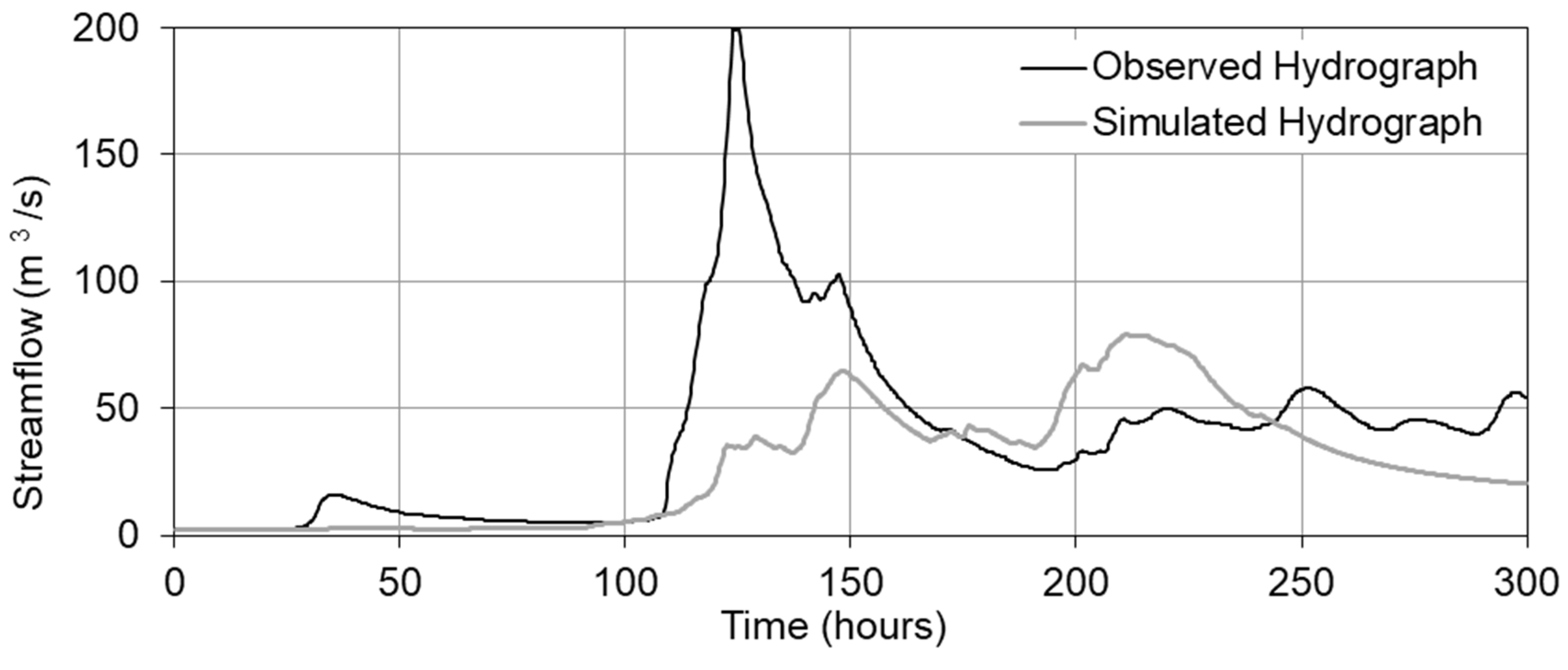
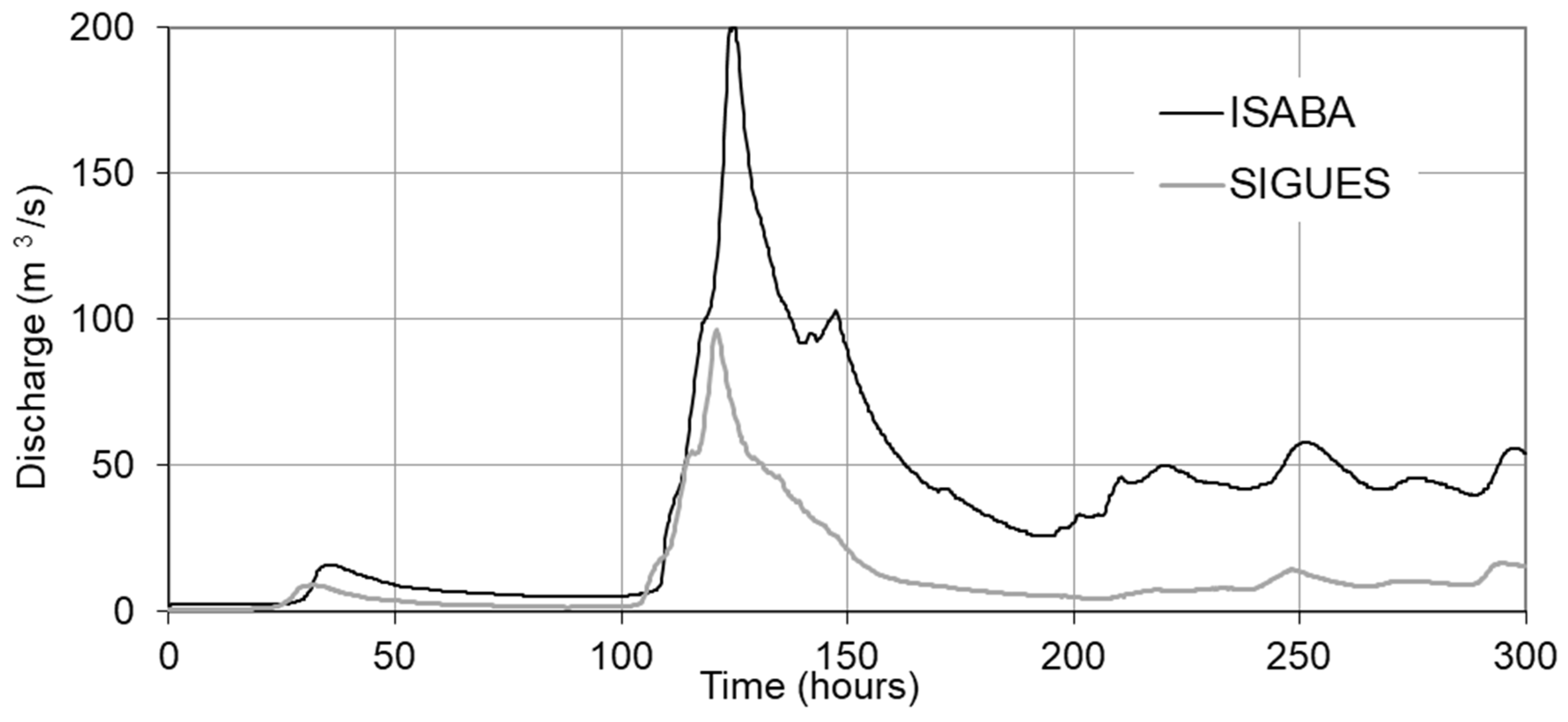
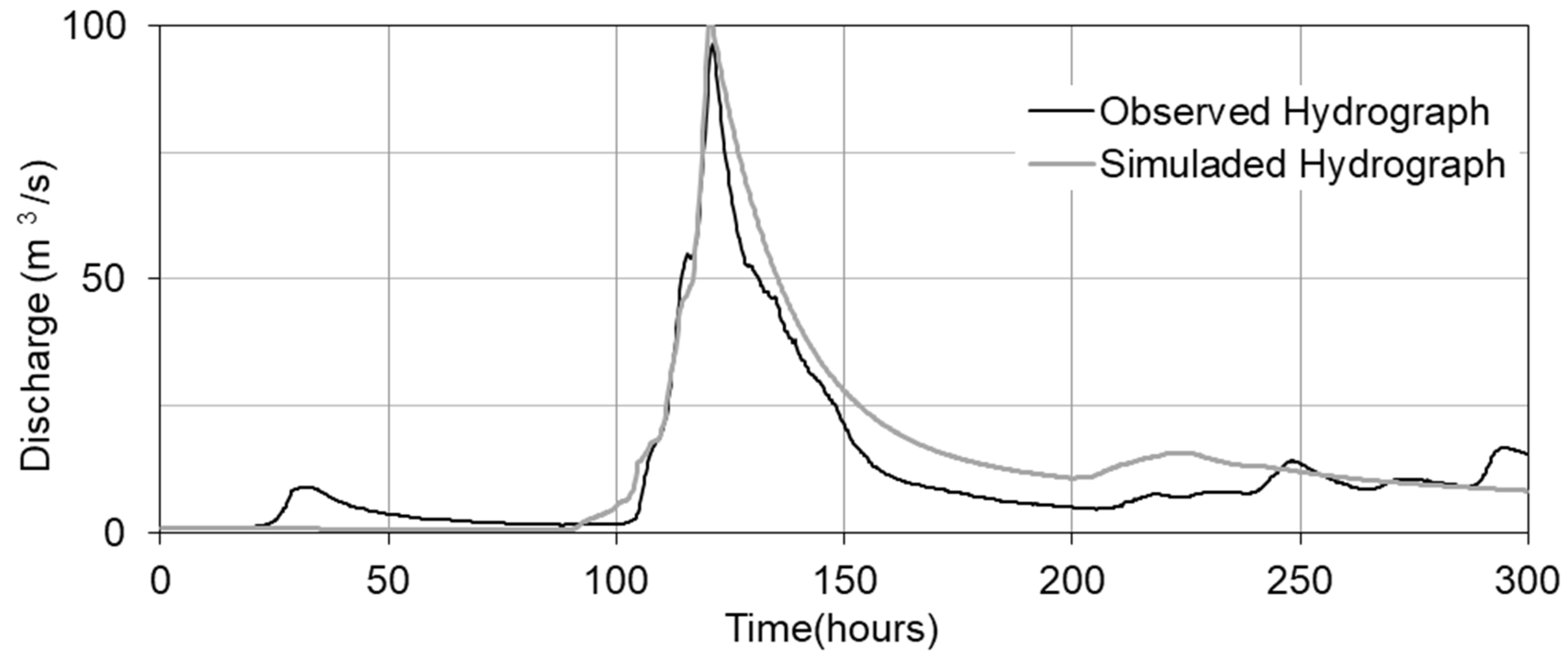
4.1. Simulation without Snowmelt
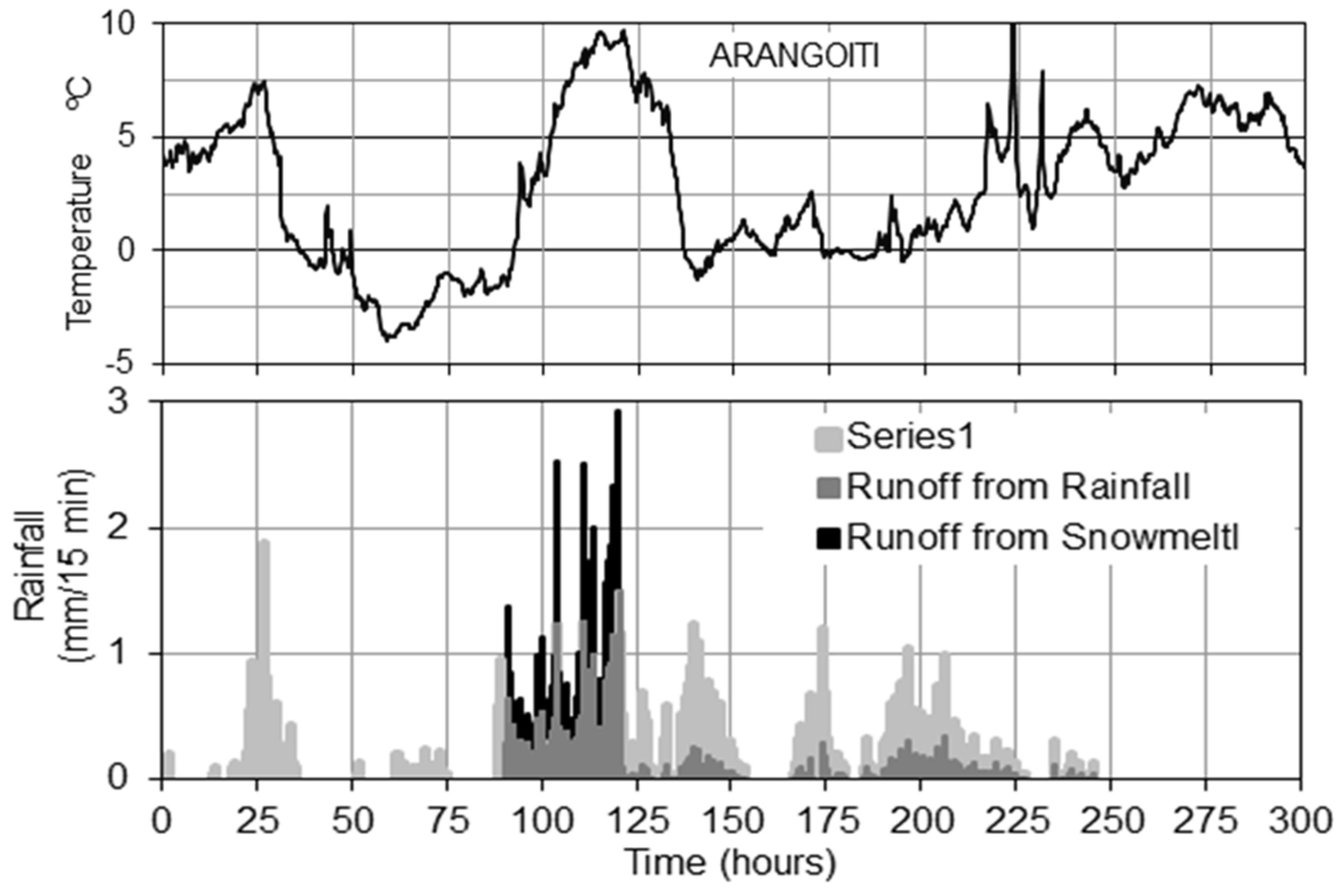
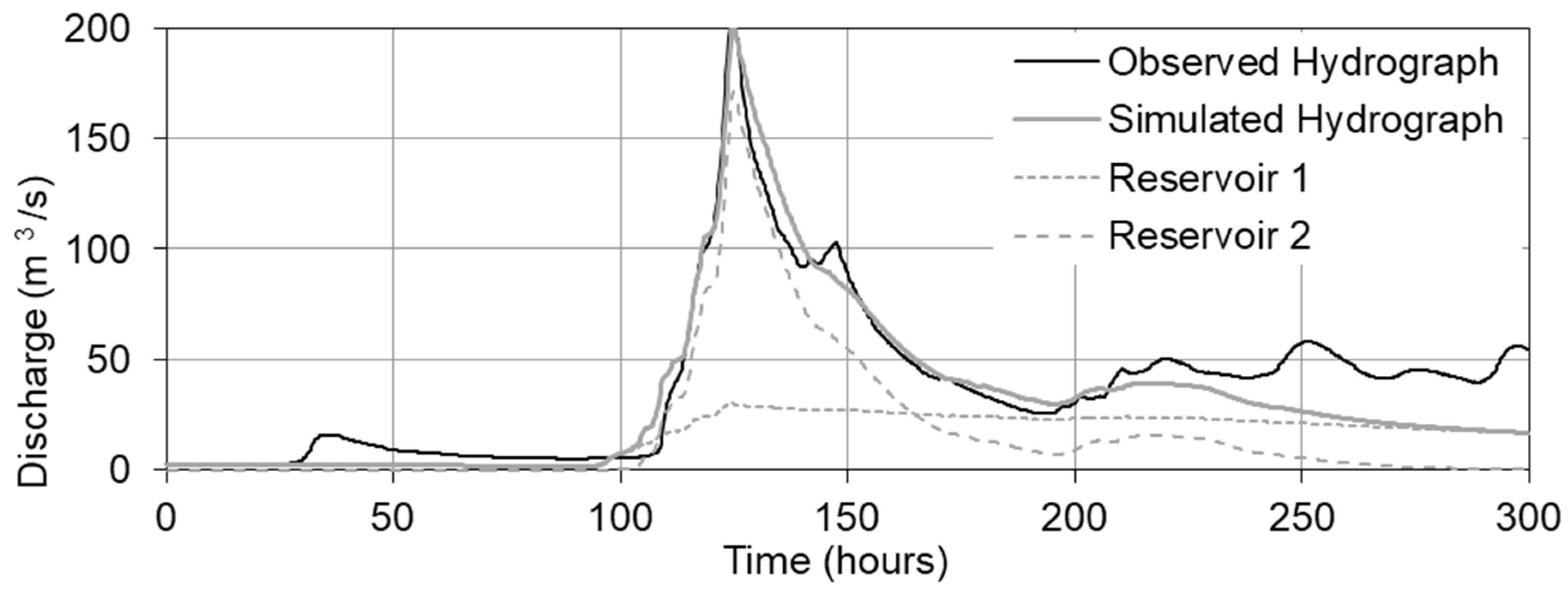
4.2. Simulation with Snowmelt
4.3. Water Budget
5. Conclusions
Author Contributions
Funding
Acknowledgments
Conflicts of Interest
References
- Duan, Y.C.; Liu, T.; Meng, F.H.; Luo, M.; Frankl, A.; De Maeyer, P.; Bao, A.; Kurban, A.; Feng, X.W. Inclusion of Modified Snow Melting and Flood Processes in the SWAT Model. Water 2018, 10, 1715. [Google Scholar] [CrossRef]
- Steimke, A.L.; Han, B.S.; Brandt, J.S.; Flores, A.N. Climate Change and Curtailment: Evaluating Water Management Practices in the Context of Changing Runoff Regimes in a Snowmelt-Dominated Basin. Water 2018, 10, 1490. [Google Scholar] [CrossRef]
- Shen, Y.J.; Shen, Y.; Fink, M.; Kralisch, S.; Chen, Y.; Brenning, A. Trends and variability in streamflow and snowmelt runoff timing in the southern Tianshan Mountains. J. Hydrol. 2018, 557, 173–181. [Google Scholar] [CrossRef]
- Dudley, R.W.; Hodgkins, G.A.; McHale, M.R.; Kolian, M.J.; Renard, M.J. Trends in snowmelt-related streamflow timing in the conterminous United States. J. Hydrol. 2017, 547, 208–221. [Google Scholar] [CrossRef]
- Penna, D.; van Meerveld, H.J.; Zuecco, G.; Dalla Fontana, G.; Borga, M. Hydrological response of an Alpine catchment to rainfall and snowmelt events. J. Hydrol. 2016, 537, 382–397. [Google Scholar] [CrossRef]
- Vormoor, K.; Lawrence, D.; Schlichting, L.; Wilson, D.; Wong, W.K. Evidence for changes in the magnitude and frequency of observed rainfall vs. snowmelt driven floods in Norway. J. Hydrol. 2016, 538, 33–48. [Google Scholar] [CrossRef]
- Kult, J.; Choi, W.; Choi, J. Sensitivity of the Snowmelt Runoff Model to snow covered area and temperature inputs. Appl. Geogr. 2014, 55, 30–38. [Google Scholar] [CrossRef]
- Driscoll, J.M.; Meixner, T.; Molotch, N.P.; Ferre, T.P.A.; Williams, M.W.; Sickman, J.O. Event-Response Ellipses: A Method to Quantify and Compare the Role of Dynamic Storage at the Catchment Scale in Snowmelt-Dominated Systems. Water 2018, 10, 1824. [Google Scholar] [CrossRef]
- Duan, L.L.; Cai, T.J. Changes in Magnitude and Timing of High Flows in Large Rain-DominatedWatersheds in the Cold Region of North-Eastern China. Water 2018, 10, 1658. [Google Scholar] [CrossRef]
- Littell, J.S.; McAfee, A.A.; Hayward, G.D. Alaska Snowpack Response to Climate Change: Statewide Snowfall Equivalent and Snowpack Water Scenarios. Water 2018, 10, 668. [Google Scholar] [CrossRef]
- Kienzle, S.W. A new temperature based method to separate rain and snow. Hydrol. Process. 2008, 22, 5067–5085. [Google Scholar] [CrossRef]
- Legates, D.R.; Bogart, T.A.; Legates, D.R.; Bogart, T.A. Estimating the Proportion of Monthly Precipitation that Falls in Solid Form. J. Hydrometeorol. 2009, 10, 1299–1306. [Google Scholar] [CrossRef]
- Pistocchi, A.; Bagli, A.; Callegari, M.; Notarnicola, C.; Mazzoli, P. On the Direct Calculation of Snow Water Balances Using Snow Cover Information. Water 2017, 9, 848. [Google Scholar] [CrossRef]
- DeBeer, C.M.; Pomeroy, J.W. Influence of snowpack and melt energy heterogeneity on snow cover depletion and snowmelt runoff simulation in a cold mountain environment. J. Hydrol. 2017, 553, 199–213. [Google Scholar] [CrossRef]
- Xie, S.P.; Du, J.; Zhou, X.B.; Zhang, X.L.; Feng, X.Z.; Zheng, W.L.; Li, Z.G.; Xu, C.Y. A progressive segmented optimization algorithm for calibrating time-variant parameters of the snowmelt runoff model (SRM). J. Hydrol. 2018, 566, 470–483. [Google Scholar] [CrossRef]
- Banasik, K.; Hejduk, A. Ratio of basin lag times for runoff and sediment yield processes recorded in various environments. Sedim. Dyn. Summit Sea Publ. IAHS 2014, 367, 163–169. [Google Scholar] [CrossRef]
- Hejduk, A.; Banasik, K. Recorded lag times of snowmelt events in a small catchment. Ann. Wars. Univ. Life Sci. SGGW Land RECLAM 2011, 43, 37–46. [Google Scholar] [CrossRef] [Green Version]
- Meng, X.; Ji, X.; Liu, Z.; Xiao, J.; Chen, X.; Wang, F. Research on Improvement and Application of Snowmelt Module in Swat. J. Nat. Resour. 2014, 29, 528–539. [Google Scholar]
- Flynn, K.F. Evaluation of Swat for Sediment Prediction in a Mountainous Snowmelt-Dominated Catchment. Trans. ASABE 2011, 54, 113–122. [Google Scholar] [CrossRef]
- Kim, S.B.; Shin, H.J.; Park, M.; Kim, S.J. Assessment of Future Climate Change Impacts on Snowmelt and Stream Water Quality for a Mountainous High-Elevation Watershed Using Swat. Paddy Water Environ. 2015, 13, 557–569. [Google Scholar] [CrossRef]
- Zhang, X.Y.; Jia, L.I.; Yang, Y.Z.; You, Z. Runoff Simulation of the Catchment of the Headwaters of the Yangtze River Based on Swat Model. J. Northwest For. Univ. 2012, 5, 9. [Google Scholar]
- Yu, W.; Zhao, Y.; Nan, Z.; Li, S. Improvement of Snowmelt Implementation in the Swat Hydrologic Model. Acta Ecol. Sin. 2013, 33, 6992–7001. [Google Scholar]
- Arnold, J.G.; Fohrer, N. Swat2000: Current Capabilities and Research Opportunities in Applied Watershed Modelling. Hydrol. Process. 2005, 19, 563–572. [Google Scholar] [CrossRef]
- Fontaine, T.A.; Cruickshank, T.S.; Arnold, J.G.; Hotchkiss, R.H. Development of a Snowfall–Snowmelt Routine for Mountainous Terrain for the SoilWater Assessment Tool (SWAT). J. Hydrol. 2002, 262, 209–223. [Google Scholar] [CrossRef]
- Wang, X.; Melesse, A.M. Evaluation of the Swat Model’s Snowmelt Hydrology in a Northwestern Minnesota Watershed. Trans. ASABE 2005, 48, 1359–1376. [Google Scholar] [CrossRef]
- Fuka, D.R.; Easton, Z.M.; Brooks, E.S.; Boll, J.; Steenhuis, T.S.; Walter, M.T. A Simple Process-Based Snowmelt Routine to Model Spatially Distributed Snow Depth and Snowmelt in the Swat Model. JAWRA J. Am. Water Resour. Assoc. 2012, 48, 1151–1161. [Google Scholar] [CrossRef]
- Green, C.H.; Van Griensven, A. Autocalibration in Hydrologic Modeling: Using Swat2005 in Small-Scale Watersheds. Environ. Model. Softw. 2008, 23, 422–434. [Google Scholar] [CrossRef]
- Ahl, R.S.; Woods, S.W.; Zuuring, H.R. Hydrologic Calibration and Validation of Swat in a Snow-Dominated Rocky Mountain Watershed, Montana, USA. JAWRA J. Am. Water Resour. Assoc. 2010, 44, 1411–1430. [Google Scholar] [CrossRef]
- Haq, M. Snowmelt Runoff Investigation in River Swat Upper Basin Using Snowmelt Runoff Model, Remote Sensing and GIS Techniques; The International Institute for Geo-information Science and Earth: Enschede, The Netherlands, 2008. [Google Scholar]
- Ficklin, D.L.; Barnhart, B.L. Corrigendum to “Swat Hydrologic Model Parameter Uncertainty and Its Implications for Hydroclimatic Projections in Snowmelt-Dependent Watersheds. J. Hydrol. 2015, 527, 1189. [Google Scholar] [CrossRef]
- Dahri, Z.H.; Ahmad, B.; Leach, J.H.; Ahmad, S. Satellite-Based Snowcover Distribution and Associated Snowmelt Runoff Modeling in Swat River Basin of Pakistan. Proc. Pak. Acad. Sci. 2011, 48, 19–32. [Google Scholar]
- Zhou, Z.; Bi, Y. Improvement of Swat Model and Its Application in Simulation of Snowmelt Runoff. In Proceedings of the National Symposium on ICE Engineering, Hohhot, China, 1 July 2011. [Google Scholar]
- Sexton, A.M.; Sadeghi, A.M.; Zhang, X.; Srinivasan, R.; Shirmohammadi, A. Using Nexrad and Rain Gauge Precipitation Data for Hydrologic Calibration of Swat in a Northeastern Watershed. Trans. ASABE 2010, 53, 1501–1510. [Google Scholar] [CrossRef]
- Martinec, J.; Rango, A. Parameter values for snowmelt runoff modeling. J. Hydrol. 1986, 84, 197–219. [Google Scholar] [CrossRef]
- Corripio, J.G.; López-Moreno, J.I. Analysis and Predictability of the Hydrological Response of Mountain Catchments to Heavy Rain on Snow Events: A Case Study in the Spanish Pyrenees. Hydrology 2017, 4, 20. [Google Scholar] [CrossRef]
- Berezowski, T.; Chybicki, A. High-Resolution Discharge Forecasting for Snowmelt and Rainfall Mixed Events. Water 2018, 10, 56. [Google Scholar] [CrossRef]
- Wu, Y.Y.; Ouyang, W.; Hao, Z.C.; Yang, B.; Wang, L. Snowmelt water drives higher soil erosion than rainfall water in a mid-high latitude upland watershed. J. Hydrol. 2018, 556, 438–448. [Google Scholar] [CrossRef]
- Starkloff, T.; Hessel, R.; Stolte, J.; Ritsema, C. Catchment Hydrology during Winter and Spring and the Link to Soil Erosion: A Case Study in Norway. Hydrology 2017, 4, 15. [Google Scholar] [CrossRef]
- Hansen, N.C.; Gupta, S.C.; Moncrief, J.F. Snowmelt runoff, sediment, and phosphorous losses under three different tillage systems. Soil Tillage Res. 2000, 57, 93–100. [Google Scholar] [CrossRef]
- Govers, G. Rill erosion on arable land in central Belgium: Rates, controls and predictability. Catena 1991, 18, 133–155. [Google Scholar] [CrossRef]
- Boardman, J.; Shepheard, M.L.; Walker, E.; Foster, I.D.L. Soil erosion risk-assessment for on- and off-farm impacts: A test case using the Midhurst area, West Sussex, UK. J. Environ. Manag. 2009, 90, 2578–2588. [Google Scholar] [CrossRef] [PubMed]
- Weigert, A.; Schmidt, J. Water transport under winter conditions. Catena 2005, 64, 193–208. [Google Scholar] [CrossRef]
- Yakutina, O.P.; Nechaeva, T.V.; Smirnova, N.V. Consequences of snowmelt erosion: Soil fertility, productivity and quality of wheat on Greyzemic Phaeozem in the south of West Siberia. Agric. Ecosyst. Environ. 2015, 200, 88–93. [Google Scholar] [CrossRef]
- Su, J.J.; van Bochove, E.; Thériault, G.; Novotma, B.; Khaldoune, J.; Denault, J.T.; Zhou, J.; Nolin, M.C.; Hu, C.X.; Bernier, M.; et al. Effects of snowmelt on phosphorus and sediment losses from agricultural watersheds in Eastern Canada. Agric. Water Manag. 2011, 98, 867–876. [Google Scholar] [CrossRef]
- Rivera, J.A.; Penalba, O.C.; Villalba, R.; Araneo, D.C. Spatio-Temporal Patterns of the 2010–2015 Extreme Hydrological Drought across the Central Andes, Argentina. Water 2017, 9, 652. [Google Scholar] [CrossRef]
- Stock, M.N.; Arriaga, F.J.; Vadas, P.A.; Karthikeyan, K.G. Manure application timing drives energy absorption for snowmelt on an agricultural soil. J. Hydrol. 2019, 569, 51–60. [Google Scholar] [CrossRef]
- Mateo-Lázaro, J.; Sánchez-Navarro, J.A.; García-Gil, A.; Edo-Romero, V. A new adaptation of linear reservoir models in parallel sets to assess actual hydrological events. J. Hydrol. 2015, 524, 507–521. [Google Scholar] [CrossRef]
- Mateo-Lázaro, J.; Castillo-Mateo, J.; Sánchez-Navarro, J.A.; Fuertes-Rodríguez, V.; García-Gil, A.; Edo-Romero, V. New Analysis Method for Continuous Base-Flow and Availability of Water Resources Based on Parallel Linear Reservoir Models. Water 2018, 10, 465. [Google Scholar] [CrossRef]
- Moore, R.D. Storage-outflow modelling of streamflow recessions, with application to a shallow-soil forested catchment. J. Hydrol. 1997, 98, 260–270. [Google Scholar] [CrossRef]
- Griffiths, G.A.; Clausen, B. Streamflow recession in basins with multiple water storages. J. Hydrol. 1997, 190, 60–74. [Google Scholar] [CrossRef]
- Dewandel, B.; Lachassagne, P.; Bakalowicz, M.; Weng, P.H.; Al-Malki, A. Evaluation of aquifer thickness by analysing recession hydrographs. Application to the Oman ophiolite hard-rock aquifer. J. Hydrol. 2003, 274, 248–269. [Google Scholar] [CrossRef]
- Smakhtin, V.Y. Low flow hydrology: A review. J. Hydrol. 2001, 240, 147–186. [Google Scholar] [CrossRef]
- Hejduk, L.; Hejduk, A.; Banasik, K. Determination of Curve Number for snowmelt-runoff floods in a small catchment. Chang. Flood Risk Percept. Catchments Cities 2015, 370, 167–170. [Google Scholar] [CrossRef] [Green Version]
- Boyd, M.J. A storage-routing model relating drainage basin hydrology and geomorphology. Water Resour. Res. 1978, 14, 921–928. [Google Scholar] [CrossRef]
- López, J.J.; Gimena, F.N.; Goñi, M.Y.; Aguirre, U. Analysis of a unit hydrograph model based on watershed geomorphology represented as a cascade of reservoirs. Agric. Water Manag. 2005, 77, 128–143. [Google Scholar] [CrossRef]
- Mateo-Lázaro, J.; Sánchez-Navarro, J.A.; García-Gil, A.; Edo-Romero, V. Developing and programming a watershed traversal algorithm (WTA) in GRID-DEM and adapting it to hydrological processes. Comput. Geosci. 2013, 51, 418–429. [Google Scholar] [CrossRef]
- Mateo-Lázaro, J.; Sánchez-Navarro, J.A.; García-Gil, A.; Edo-Romero, V. Sensitivity analysis of main variables present on flash flood processes. Application in two Spanish catchments: Arás and Aguilón. Environ. Earth Sci. 2014, 71, 2925–2939. [Google Scholar] [CrossRef]
- Mateo-Lázaro, J.; Sánchez-Navarro, J.A.; García-Gil, A.; Edo-Romero, V. 3D-geological structures with digital elevation models using GPU programming. Comput. Geosci. 2014, 70, 147–153. [Google Scholar] [CrossRef]
- García-Gil, A.; Vázquez-Suñé, E.; Sánchez-Navarro, J.A.; Mateo-Lázaro, J. Recovery of energetically overexploited urban aquifers using Surface water. J. Hydrol. 2015, 531, 602–611. [Google Scholar] [CrossRef]
- García-Gil, A.; Vázquez-Suñé, E.; Sánchez-Navarro, J.A.; Mateo-Lázaro, J.; Alcaraz, M. The propagation of complex flood-induced head wavefronts through a heterogeneous alluvial aquifer and its applicability in groundwater flood risk management. J. Hydrol. 2015, 527, 402–419. [Google Scholar] [CrossRef]
- Mateo-Lázaro, J.; Sánchez-Navarro, J.A.; García-Gil, A.; Edo-Romero, V. Flood Frequency Analysis (FFA) in Spanish catchments. J. Hydrol. 2016, 538, 598–608. [Google Scholar] [CrossRef]
- Mateo-Lázaro, J.; Sánchez-Navarro, J.A.; García-Gil, A.; Edo-Romero, V.; Castillo-Mateo, J. Modelling and layout of drainage-levee devices in river sections. Eng. Geol. 2016, 214, 11–19. [Google Scholar] [CrossRef]
- García-Gil, A.; Epting, J.; Garrido, E.; Vázquez-Suñé, E.; Mateo-Lázaro, J.; Sánchez Navarro, J.A.; Huggenberger, P.; Marazuela Calvo, M.A. A city scale study on the effects of intensive groundwater heat pump systems on heavy metal contents in groundwater. Sci. Total Environ. 2016, 572, 1047–1058. [Google Scholar] [CrossRef] [PubMed]
- Mateo-Lázaro, J.; Sánchez-Navarro, J.A.; García-Gil, A.; Edo-Romero, V. SHEE program, a tool for the display, analysis and interpretation of hydrological processes in watersheds. In Lecture Notes in Earth System Sciences, Mathematics of Planet Earth, Proceedings of the 15th Annual Conference of the International Association for Mathematical Geosciences; Springer: Berlin/Heidelberg, Germany, 2014; pp. 303–307. [Google Scholar]
- Mateo-Lázaro, J.; Sánchez-Navarro, J.A.; Edo-Romero, V.; García-Gil, A. Models of parallel linear reservoirs (PLR) with watershed traversal algorithm (WTA) in behaviour research of hydrological processes in catchments. In Lecture Notes in Earth System Sciences, Mathematics of Planet Earth, Proceedings of the 15th Annual Conference of the International Association for Mathematical Geosciences; Springer: Berlin/Heidelberg, Germany, 2014; pp. 471–474. [Google Scholar]
- Tayyab, M.; Ahmad, I.; Sun, N.; Zhou, J.; Dong, X. Application of Integrated Artificial Neural Networks Based on Decomposition Methods to Predict Streamflow at Upper Indus Basin, Pakistan. Atmosphere 2018, 9, 494. [Google Scholar] [CrossRef]
- Koycegiz, C.; Buyukyildiz, M. Calibration of SWAT and Two Data-Driven Models for a Data-Scarce Mountainous Headwater in Semi-Arid Konya Closed Basin. Water 2019, 11, 147. [Google Scholar] [CrossRef]
- Ma, M.; Liu, C.; Zhao, G.; Xie, H.; Jia, P.; Wang, D.; Wang, H.; Hong, Y. Flash Flood Risk Analysis Based on Machine Learning Techniques in the Yunnan Province, China. Remote Sens. 2019, 11, 170. [Google Scholar] [CrossRef]


| Characteristic | ud | Isaba (A268) | Sigues (A063) |
|---|---|---|---|
| Catchment area | km2 | 189.06 | 506.26 |
| Length of the main channel | km | 24.01 | 51.70 |
| Average slope of the main channel | % | 6.44 | 3.45 |
| Average slope of the digital surface of the catchment | % | 36.85 | 34.88 |
| Average curve number (AMC II) | 63.08 | 61.22 |
| Date | Rain Duration (h) | Time Interval (15 min) | Peak Flow(m3/s) | |
|---|---|---|---|---|
| Start Time | End Time | |||
| 2:30 p.m. 18 January 2009 | 7:30 p.m. 28 January 2009 | 245.25 | 981 | 201 |
| Parameter | Reservoir | |
|---|---|---|
| 1 | 2 | |
| a → | 1.43 × 10⁻⁶ | 1.67 × 10⁻⁵ |
| q0 → | 2.96 × 10⁻⁷ | 1.00 |
| Acronym | Tilte | Isaba hm3 | Sigues hm3 | Isaba mm | Sigues mm | Isaba/Sigues % |
|---|---|---|---|---|---|---|
| Tp | Total precipitation | 31.79 | 67.61 | 168 | 134 | 127% |
| Tr | Total runoff | 17.90 | 42.06 | 95 | 83 | 90% |
| Ep | Effective precipitation | 11.47 | 19.27 | 61 | 38 | 101% |
| Sm | Snowmelt | 6.43 | 22.79 | 34 | 45 | 76% |
| L | Losses | 20.32 | 48.33 | 107 | 95 | 148% |
| Hv * | Hydrograph volume | 9.80 | 25.86 | 52 | 51 | 80% |
© 2019 by the authors. Licensee MDPI, Basel, Switzerland. This article is an open access article distributed under the terms and conditions of the Creative Commons Attribution (CC BY) license (http://creativecommons.org/licenses/by/4.0/).
Share and Cite
Mateo-Lázaro, J.; Castillo-Mateo, J.; Sánchez-Navarro, J.Á.; Fuertes-Rodríguez, V.; García-Gil, A.; Edo-Romero, V. Assessment of the Role of Snowmelt in a Flood Event in a Gauged Catchment. Water 2019, 11, 506. https://doi.org/10.3390/w11030506
Mateo-Lázaro J, Castillo-Mateo J, Sánchez-Navarro JÁ, Fuertes-Rodríguez V, García-Gil A, Edo-Romero V. Assessment of the Role of Snowmelt in a Flood Event in a Gauged Catchment. Water. 2019; 11(3):506. https://doi.org/10.3390/w11030506
Chicago/Turabian StyleMateo-Lázaro, Jesús, Jorge Castillo-Mateo, José Ángel Sánchez-Navarro, Víctor Fuertes-Rodríguez, Alejandro García-Gil, and Vanesa Edo-Romero. 2019. "Assessment of the Role of Snowmelt in a Flood Event in a Gauged Catchment" Water 11, no. 3: 506. https://doi.org/10.3390/w11030506