Novel Hybrid Data-Intelligence Model for Forecasting Monthly Rainfall with Uncertainty Analysis

 ,
,  ,
,  , , , ,
  and
and 
Abstract
:1. Introduction
2. Methodology
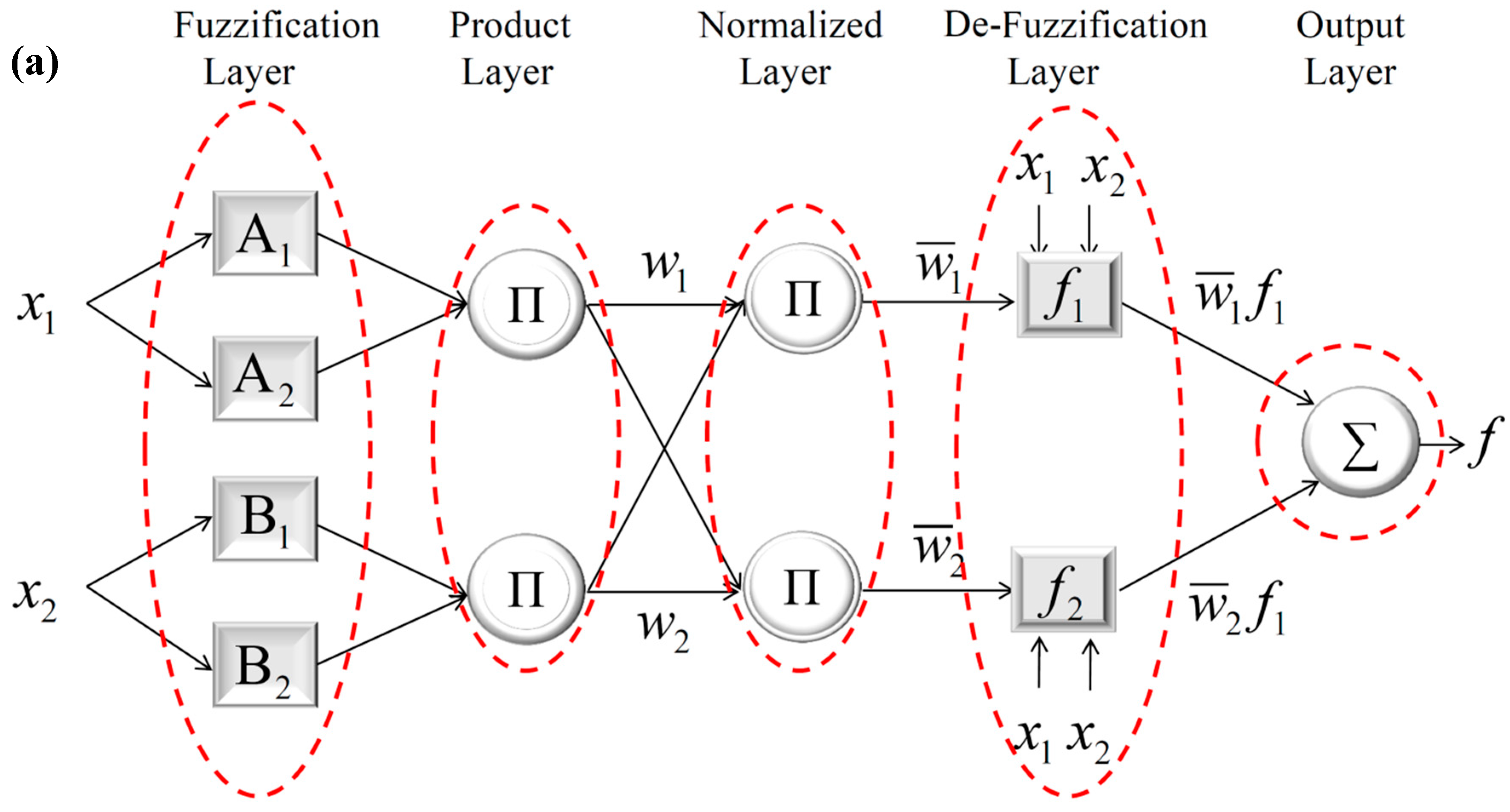
2.1. Adaptive Neuro-Fuzzy Inference System
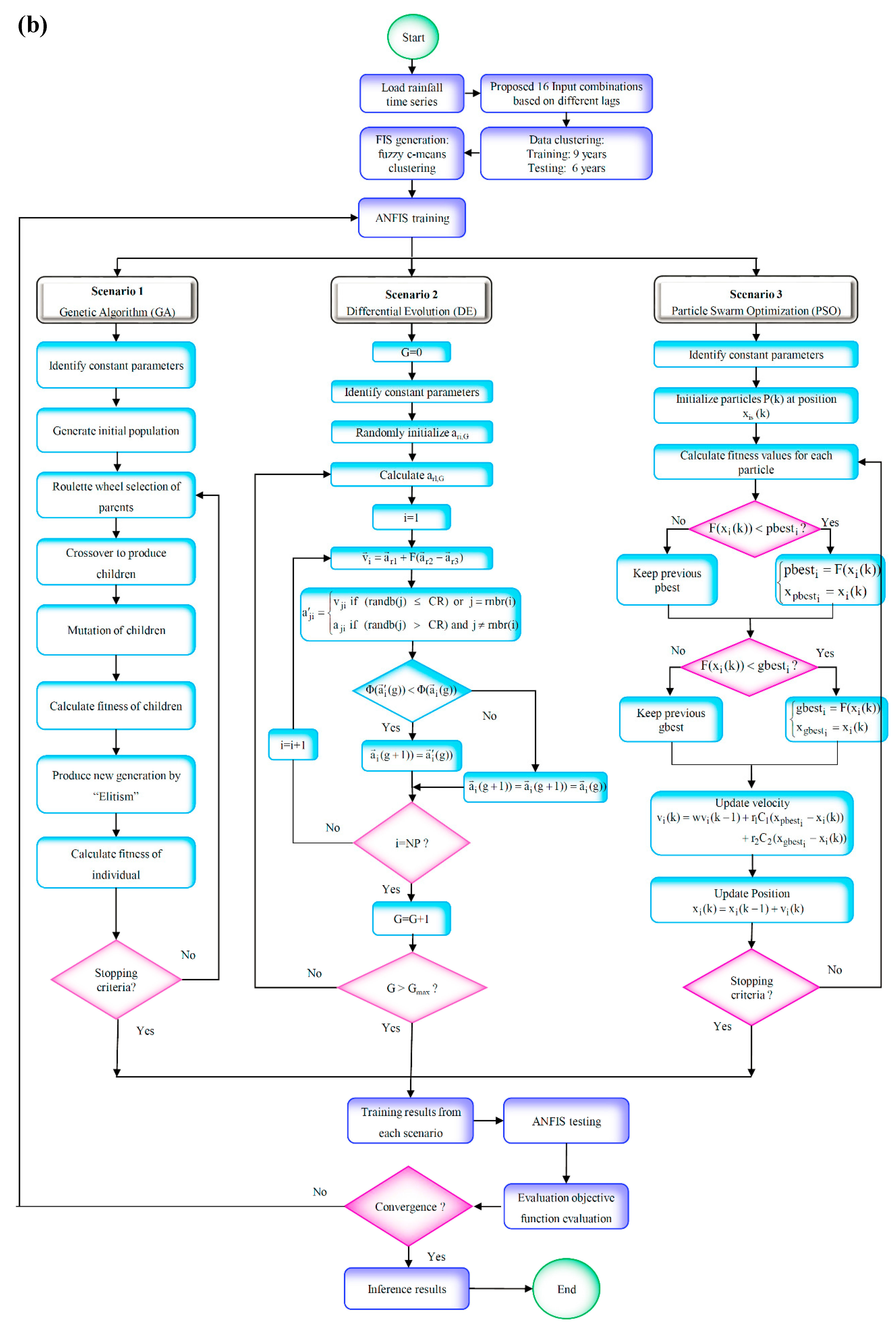
2.2. Particle Swarm Optimization (PSO)
2.3. Genetic Algorithm (GA) Optimization
2.4. Differential Evolution (DE) Optimization
2.5. Hybridization of ANFIS Model
2.6. Modeling Performance Indicators
2.7. Uncertainty Analysis
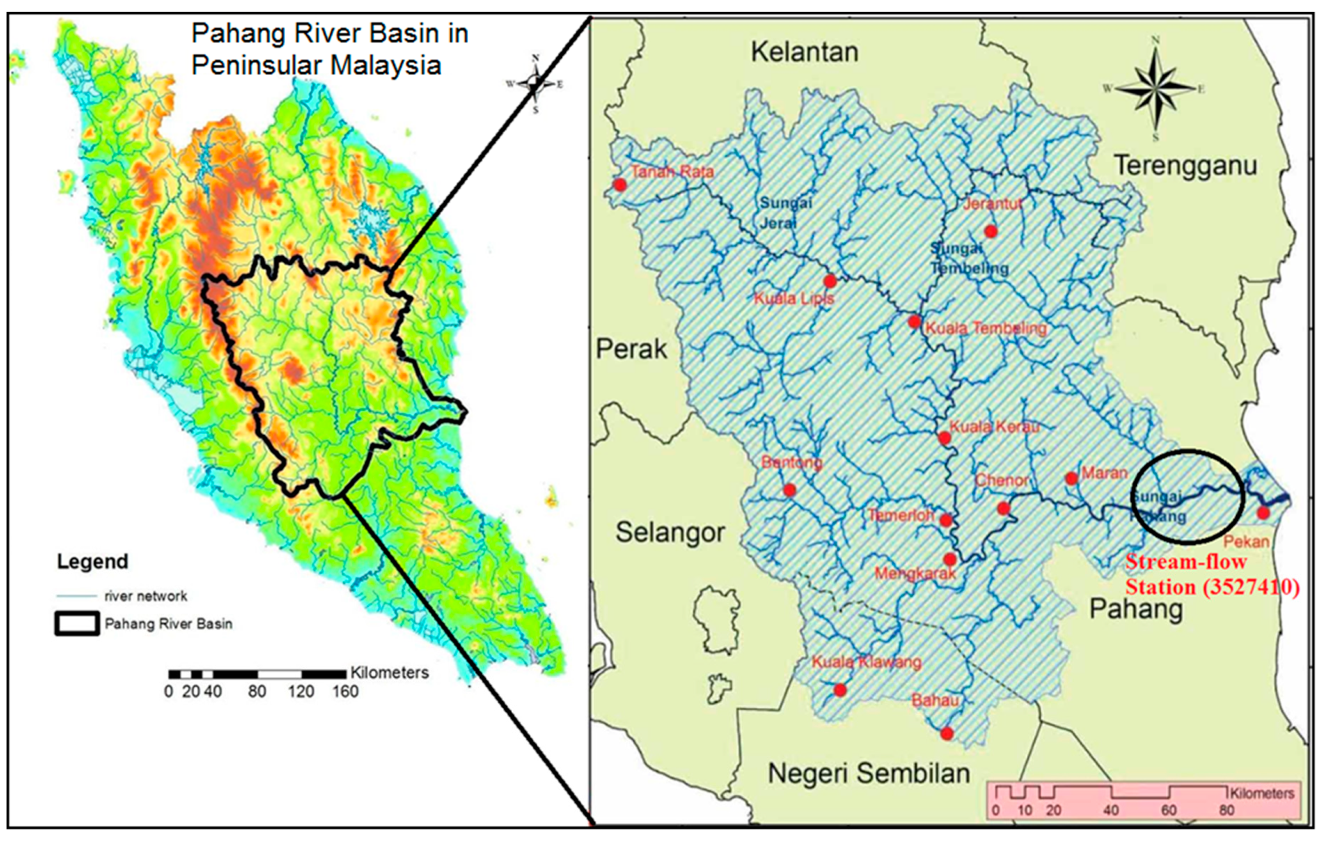
3. Case Study and Hydrological Data Description
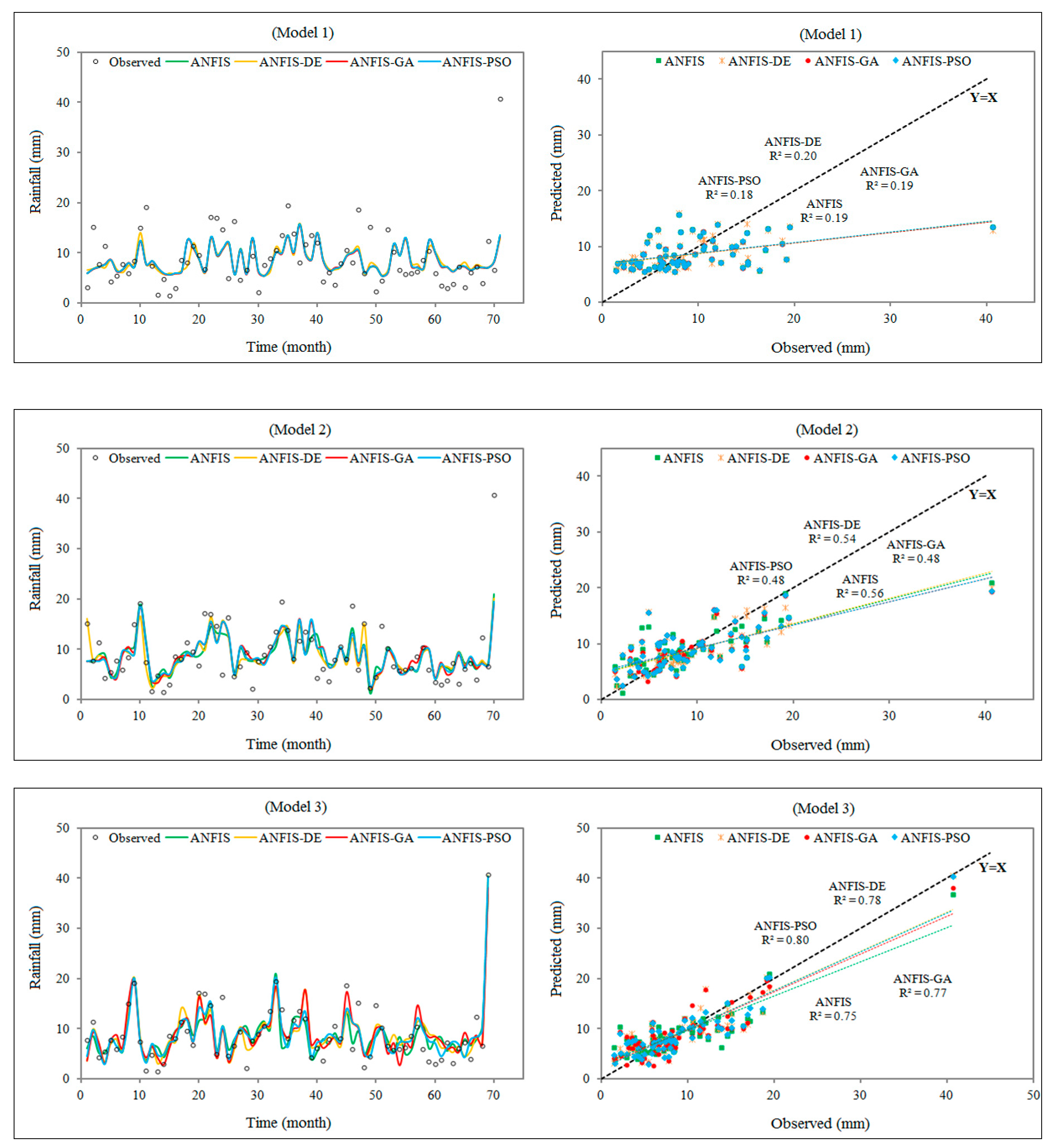
4. Application and Analysis
5. Conclusions
Author Contributions
Funding
Acknowledgments
Conflicts of Interest
References
- Vaze, J.; Post, D.A.; Chiew, F.H.S.; Perraud, J.M.; Viney, N.R.; Teng, J. Climate non-stationarity—Validity of calibrated rainfall-runoff models for use in climate change studies. J. Hydrol. 2010, 394, 447–457. [Google Scholar] [CrossRef]
- Khan, N.; Shahid, S.; Juneng, L.; Ahmed, K.; Ismail, T.; Nawaz, N. Prediction of heat waves in Pakistan using quantile regression forests. Atmos. Res. 2019. [Google Scholar] [CrossRef]
- Tripathi, S.; Govindaraju, R.S. Statistical forecasting of Indian Summer Monsoon Rainfall: An enduring challenge. Stud. Fuzziness Soft Comput. 2008, 207–224. [Google Scholar] [CrossRef]
- Wang, Q.J.; Schepen, A.; Robertson, D.E. Merging seasonal rainfall forecasts from multiple statistical models through Bayesian model averaging. J. Clim. 2012, 25, 5524–5537. [Google Scholar] [CrossRef]
- Yuan, F.; Berndtsson, R.; Uvo, C.B.; Zhang, L.; Jiang, P. Summer precipitation prediction in the source region of the Yellow River using climate indices. Hydrol. Res. 2016, 47, 847–856. [Google Scholar] [CrossRef]
- Sittichok, K.; Djibo, A.G.; Seidou, O.; Saley, H.M.; Karambiri, H.; Paturel, J. Statistical seasonal rainfall and streamflow forecasting for the Sirba watershed, West Africa, using sea-surface temperatures. Hydrol. Sci. J. 2016, 61, 805–815. [Google Scholar] [CrossRef]
- Štěpnička, M.; Cortez, P.; Donate, J.P.; Štěpničková, L. Forecasting seasonal time series with computational intelligence: On recent methods and the potential of their combinations. Expert Syst. Appl. 2013, 40, 1981–1992. [Google Scholar] [CrossRef] [Green Version]
- Pereira, P.J.; Cortez, P.; Mendes, R. Multi-objective Learning of Neural Network Time Series Prediction Intervals. In Progress in Artificial Intelligence; Springer: Cham, Switzerland, 2017; pp. 561–572. [Google Scholar]
- Deb, K. Multi-Objective Optimization Using Evolutionary Algorithms; John Wiley & Sons, LTD: West Sussex, England, 2001; p. 497. [Google Scholar]
- Liu, S.; Tai, H.; Ding, Q.; Li, D.; Xu, L.; Wei, Y. A hybrid approach of support vector regression with genetic algorithm optimization for aquaculture water quality prediction. Math. Comput. Model. 2013, 58. [Google Scholar] [CrossRef]
- Yaseen, Z.M.; Ghareb, M.I.; Ebtehaj, I.; Bonakdari, H.; Ravinesh, D.; Siddique, R.; Heddam, S.; Yusif, A. Rainfall Pattern Forecasting Using Novel Hybrid Intelligent Model Based ANFIS-FFA. Water Resour. Manag. 2017, 32, 105–122. [Google Scholar] [CrossRef]
- Nayak, P.C.; Sudheer, K.P.; Jain, S.K. Rainfall-runoff modeling through hybrid intelligent system. Water Resour. Res. 2007, 43, 1–17. [Google Scholar] [CrossRef]
- Pulido-Calvo, I.; Gutiérrez-Estrada, J.C. Improved irrigation water demand forecasting using a soft-computing hybrid model. Biosyst. Eng. 2009, 102, 202–218. [Google Scholar] [CrossRef]
- Nourani, V.; Kisi, Ö.; Komasi, M. Two hybrid Artificial Intelligence approaches for modeling rainfall-runoff process. J. Hydrol. 2011, 402, 41–59. [Google Scholar] [CrossRef]
- Abdullah, S.S.; Abdul Malek, M.; Mustapha, A.; Aryanfar, A. Hybrid of Artificial Neural Network-Genetic Algorithm for Prediction of Reference Evapotranspiration (ET0) in Arid and Semiarid Regions. J. Agric. Sci. 2014, 6, 191–200. [Google Scholar] [CrossRef]
- Abrahart, R.J.; See, L.; Kneale, P.E. Using pruning algorithms and genetic algorithms to optimise network architectures and forecasting inputs in a neural network rainfall-runoff model. J. Hydroinf. 1999, 103–114. [Google Scholar] [CrossRef]
- Chau, K.W. Particle swarm optimization training algorithm for ANNs in stage prediction of Shing Mun River. J. Hydrol. 2006, 329, 363–367. [Google Scholar] [CrossRef] [Green Version]
- Chau, K.W. A split-step particle swarm optimization algorithm in river stage forecasting. J. Hydrol. 2007, 346, 131–135. [Google Scholar] [CrossRef] [Green Version]
- Chen, Y.H.; Chang, F.J. Evolutionary artificial neural networks for hydrological systems forecasting. J. Hydrol. 2009, 367, 125–137. [Google Scholar] [CrossRef]
- Kisi, O.; Ozkan, C.; Akay, B. Modeling discharge-sediment relationship using neural networks with artificial bee colony algorithm. J. Hydrol. 2012, 428–429, 94–103. [Google Scholar] [CrossRef]
- Asadnia, M.; Chua, L.H.C.; Qin, X.S.; Talei, A. Improved Particle Swarm Optimization–Based Artificial Neural Network for Rainfall-Runoff Modeling. J. Hydrol. Eng. 2014, 19, 1320–1329. [Google Scholar] [CrossRef]
- Sudheer, C.; Maheswaran, R.; Panigrahi, B.K.; Mathur, S. A hybrid SVM-PSO model for forecasting monthly streamflow. Neural Comput. Appl. 2013, 1–9. [Google Scholar] [CrossRef]
- Taormina, R.; Chau, K. Neural network river forecasting with multi-objective fully informed particle swarm optimization. J. Hydroinf. 2015, 17, 99–112. [Google Scholar] [CrossRef]
- Kalteh, A.M. Wavelet Genetic Algorithm-Support Vector Regression (Wavelet GA-SVR) for Monthly Flow Forecasting. Water Resour. Manag. 2015, 29, 1283–1293. [Google Scholar] [CrossRef]
- Annaty, M.; Eghbalzadeh, A.; Hosseini, S. Hybrid ANFIS Model for Predicting Scour Depth using Particle Swarm Optimization. Indian J. Sci. Technol. 2015, 8, 326–332. [Google Scholar] [CrossRef]
- Yaseen, Z.M.; Ramal, M.M.; Diop, L.; Jaafar, O.; Demir, V.; Kisi, O. Hybrid Adaptive Neuro-Fuzzy Models for Water Quality Index Estimation. Water Resour. Manag. 2018, 32, 2227–2245. [Google Scholar] [CrossRef]
- Ghorbani, M.A.; Deo, R.C.; Yaseen, Z.M.; Kashani, M.H. Pan evaporation prediction using a hybrid multilayer perceptron-firefly algorithm ( MLP-FFA ) model: Case study in North Iran. Theor. Appl. Climatol. 2018, 133, 1119–1131. [Google Scholar] [CrossRef]
- Ghorbani, M.A.; Deo, R.C.; Karimi, V.; Yaseen, Z.M.; Terzi, O. Implementation of a hybrid MLP-FFA model for water level prediction of Lake Egirdir, Turkey. Stoch. Environ. Res. Risk Assess. 2018, 32, 1683–1697. [Google Scholar] [CrossRef]
- Yaseen, Z.M.; Karami, H.; Ehteram, M.; Mohd, N.S.; Mousavi, S.F.; Hin, L.S.; Kisi, O.; Farzin, S.; Kim, S.; El-shafie, A. Optimization of Reservoir Operation Using New Hybrid Algorithm. KSCE J. Civ. Eng. 2018, 22, 4668–4680. [Google Scholar] [CrossRef]
- Zadeh, L. Fuzzy Sets. Inf. Control 1965, 8, 338–353. [Google Scholar] [CrossRef]
- Takagi, T.; Sugeno, M. Fuzzy Identification of Systems and Its Applications to Modeling and Control. IEEE Trans. Syst. Man Cybern. 1985, SMC-15, 116–132. [Google Scholar] [CrossRef]
- Çekmiş, A.; Hacihasanoǧlu, I.; Ostwald, M.J. A computational model for accommodating spatial uncertainty: Predicting inhabitation patterns in open-planned spaces. Build. Environ. 2014, 73, 115–126. [Google Scholar] [CrossRef]
- Moosavi, V.; Vafakhah, M.; Shirmohammadi, B.; Behnia, N. A Wavelet-ANFIS Hybrid Model for Groundwater Level Forecasting for Different Prediction Periods. Water Resour. Manag. 2013, 27, 1301–1321. [Google Scholar] [CrossRef]
- Kennedy, J.; Eberhart, R. Particle swarm optimization. In Proceedings of the IEEE International Conference on Neural Networks, Perth, Australia, 27 November–1 December 1995; Volume 4, pp. 1942–1948. [Google Scholar] [CrossRef]
- Mirjalili, S. Genetic Algorithm. In Evolutionary Algorithms and Neural Networks; Springer: Berlin, Germany, 2019; pp. 43–55. [Google Scholar]
- Goldberg, D.E.; Holland, J.H. Genetic algorithms and machine learning. Mach. Learn. 1988, 3, 95–99. [Google Scholar] [CrossRef]
- Storn, R.; Price, K. Differential Evolution—A Simple and Efficient Heuristic for Global Optimization over Continuous Spaces. J. Glob. Optim. 1997, 11, 341–359. [Google Scholar] [CrossRef]
- Halabi, L.M.; Mekhilef, S.; Hossain, M. Performance evaluation of hybrid adaptive neuro-fuzzy inference system models for predicting monthly global solar radiation. Appl. Energy 2018, 213, 247–261. [Google Scholar] [CrossRef]
- Chai, T.; Draxler, R.R. Root mean square error (RMSE) or mean absolute error (MAE)?-Arguments against avoiding RMSE in the literature. Geosci. Model Dev. 2014, 7, 1247–1250. [Google Scholar] [CrossRef]
- Willmott, C.J.; Matsuura, K. Advantages of the mean absolute error (MAE) over the root mean square error (RMSE) in assessing average model performance. Clim. Res. 2005, 30, 79–82. [Google Scholar] [CrossRef] [Green Version]
- Willmott, C.J. On the validation of models. Phys. Geogr. 1981, 2, 184–194. [Google Scholar] [CrossRef]
- Armstrong, J.S.; Collopy, F. Error measures for generalizing about forecasting methods: Empirical comparisons. Int. J. Forecast. 1992, 8, 69–80. [Google Scholar] [CrossRef] [Green Version]
- Pandhiani, S.M. Time Series Forecasting by Using Hybrid Models for Monthly Streamflow Data. Appl. Math. Sci. 2015, 9, 2809–2829. [Google Scholar] [CrossRef]
- Yaseen, Z.M.; El-Shafie, A.; Afan, H.A.; Hameed, M.; Mohtar, W.H.M.W.; Hussain, A. RBFNN versus FFNN for daily river flow forecasting at Johor River, Malaysia. Neural Comput. Appl. 2016, 27, 1533–1542. [Google Scholar] [CrossRef]
- Afan, H.A.; Keshtegar, B.; Mohtar, W.H.M.W.; El-Shafie, A. Harmonize input selection for sediment transport prediction. J. Hydrol. 2017, 552, 366–375. [Google Scholar] [CrossRef]
- Kumar, K.K.; Soman, M.K.; Kumar, K.R. Seasonal forecasting of Indian summer monsoon rainfall: A review. Weather 1995, 50, 449–467. [Google Scholar] [CrossRef]
- Taylor, K.E. Summarizing multiple aspects of model performance in a single diagram. J. Geophys. Res. Atmos. 2001, 106, 7183–7192. [Google Scholar] [CrossRef] [Green Version]
- Heo, K.-Y.; Ha, K.-J.; Yun, K.-S.; Lee, S.-S.; Kim, H.-J.; Wang, B. Methods for uncertainty assessment of climate models and model predictions over East Asia. Int. J. Climatol. 2014, 34, 377–390. [Google Scholar] [CrossRef]
- Abbaspour, K.C.; Yang, J.; Maximov, I.; Siber, R.; Bogner, K.; Mieleitner, J.; Zobrist, J. Modelling hydrology and water quality in the pre-alpine / alpine Thur watershed using SWAT. J. Hydrol. 2007, 333, 413–430. [Google Scholar] [CrossRef]
- Jiang, P.; Gautam, M.R.; Zhu, J.; Yu, Z. How well do the GCMs/RCMs capture the multi-scale temporal variability of precipitation in the Southwestern United States? J. Hydrol. 2013, 479, 75–85. [Google Scholar] [CrossRef]
- Sato, T.; Kimura, F.; Kitoh, A. Projection of global warming onto regional precipitation over Mongolia using a regional climate model. J. Hydrol. 2007, 333, 144–154. [Google Scholar] [CrossRef]
- Hellström, C.; Chen, D.; Achberger, C.; Räisänen, J. Comparison of climate change scenarios for Sweden based on statistical and dynamical downscaling of monthly precipitation. Clim. Res. 2001, 19, 45–55. [Google Scholar] [CrossRef] [Green Version]
- Maurer, E.P.; Hidalgo, H.G. Utility of daily vs. monthly large-scale climate data: An intercomparison of two statistical downscaling methods. Hydrol. Earth Syst. Sci. 2008, 12, 551–563. [Google Scholar] [CrossRef]


| (a) ANFIS-based model | ||||||||
| Models | RMSE (mm) | MAE (mm) | CC | WI | RMSE (mm) | MAE (mm) | CC | WI |
| Training phase | Testing phase | |||||||
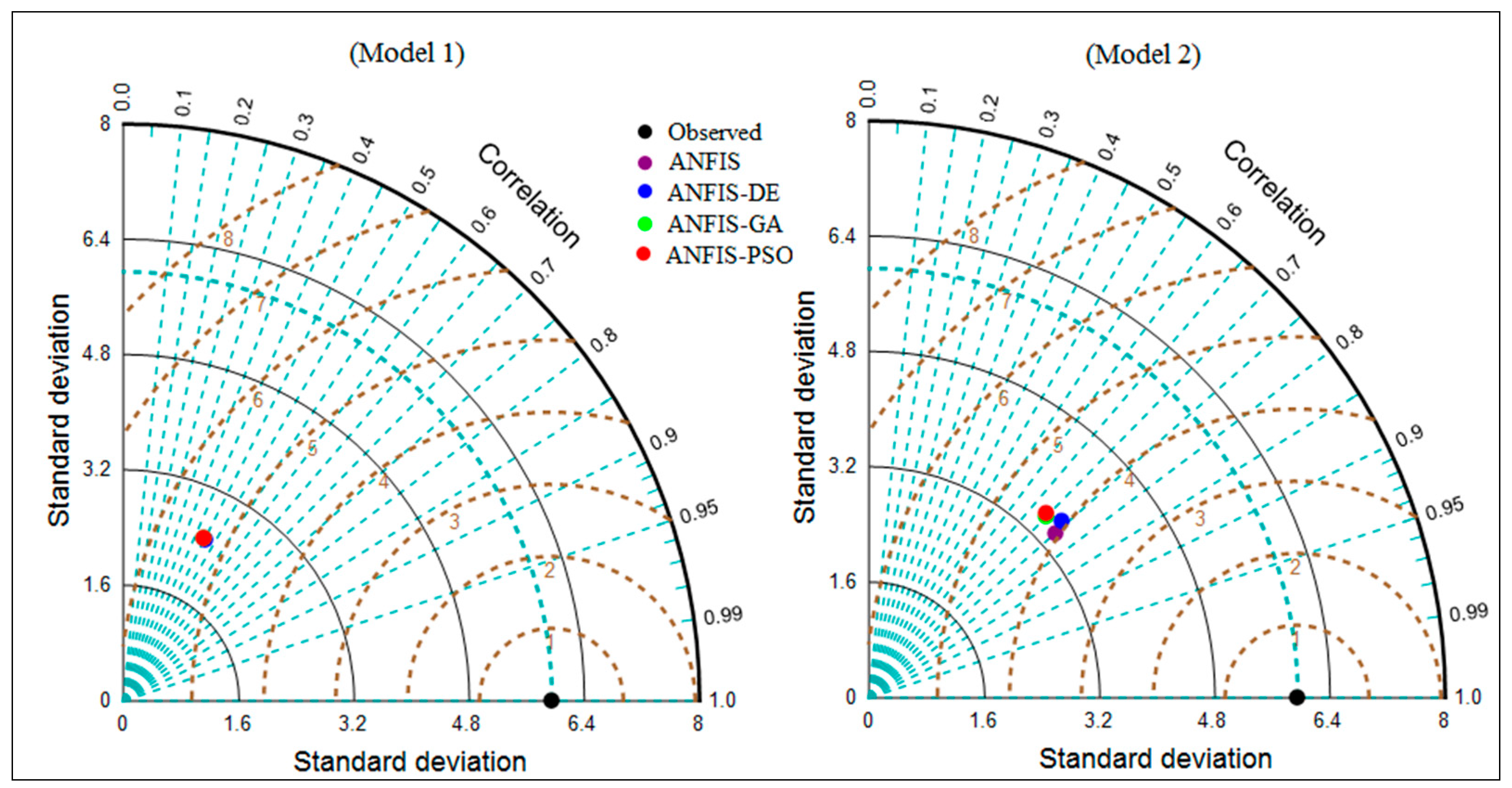
| Model 1 | 4.23 | 3.16 | 0.492 | 0.564 | 5.32 | 3.69 | 0.439 | 0.478 |
| Model 2 | 4.02 | 2.85 | 0.575 | 0.698 | 4.04 | 2.73 | 0.749 | 0.788 |
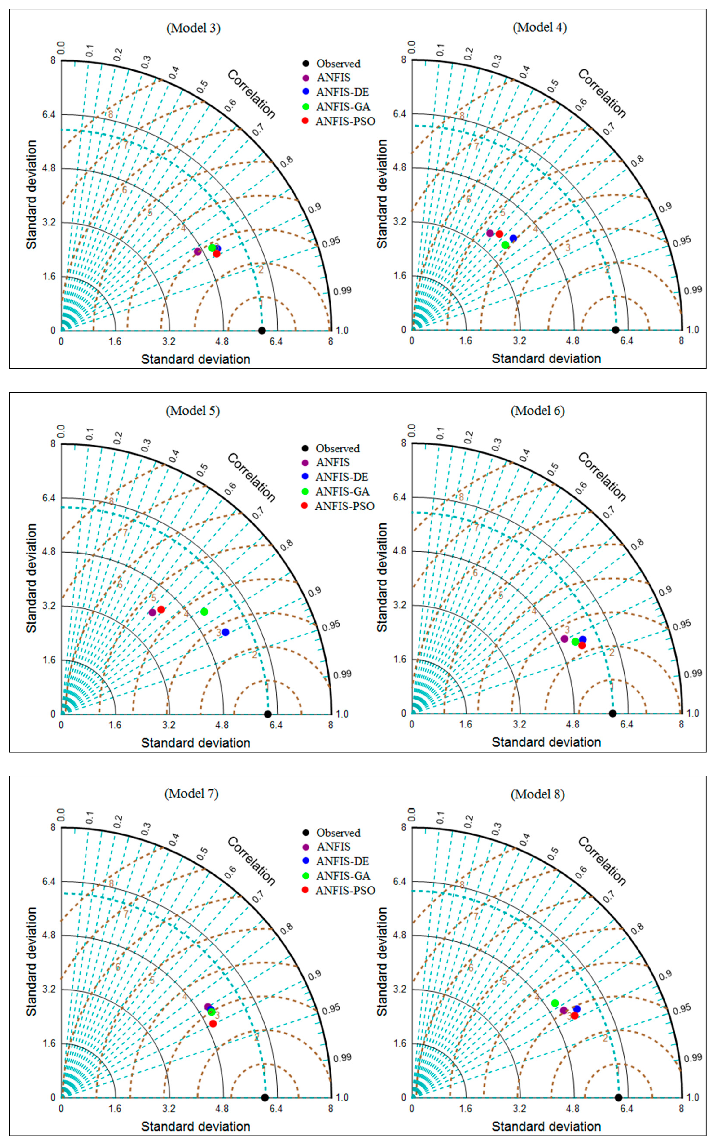
| Model 3 | 2.96 | 2.22 | 0.799 | 0.882 | 3.00 | 2.31 | 0.864 | 0.913 |
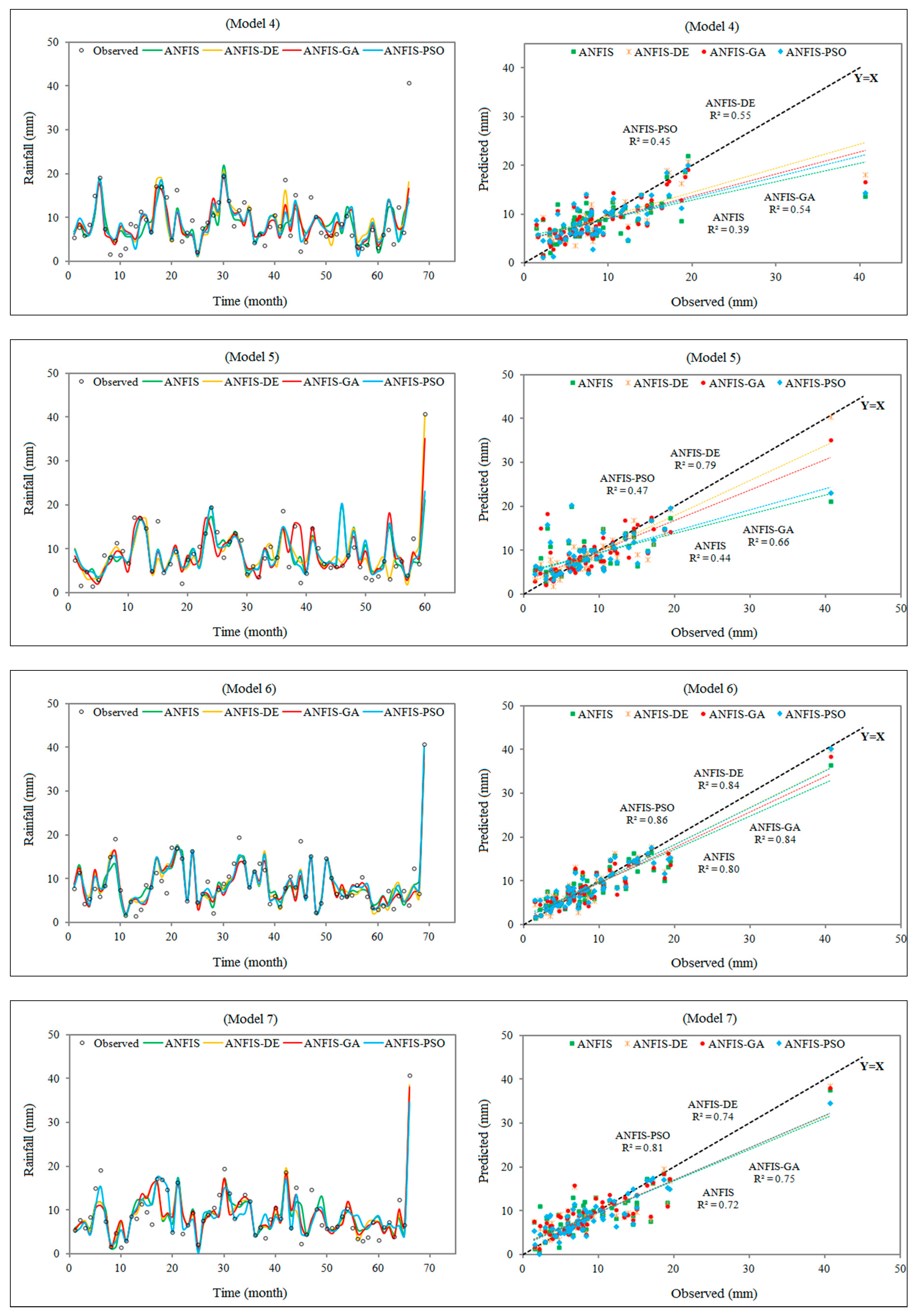
| Model 4 | 3.41 | 2.43 | 0.723 | 0.810 | 4.69 | 2.91 | 0.627 | 0.714 |
| Model 5 | 2.87 | 1.95 | 0.820 | 0.888 | 4.54 | 2.82 | 0.664 | 0.759 |
| Model 6 | 3.08 | 2.30 | 0.780 | 0.865 | 2.63 | 2.00 | 0.897 | 0.938 |
| Model 7 | 3.40 | 2.26 | 0.724 | 0.806 | 3.17 | 2.28 | 0.848 | 0.911 |
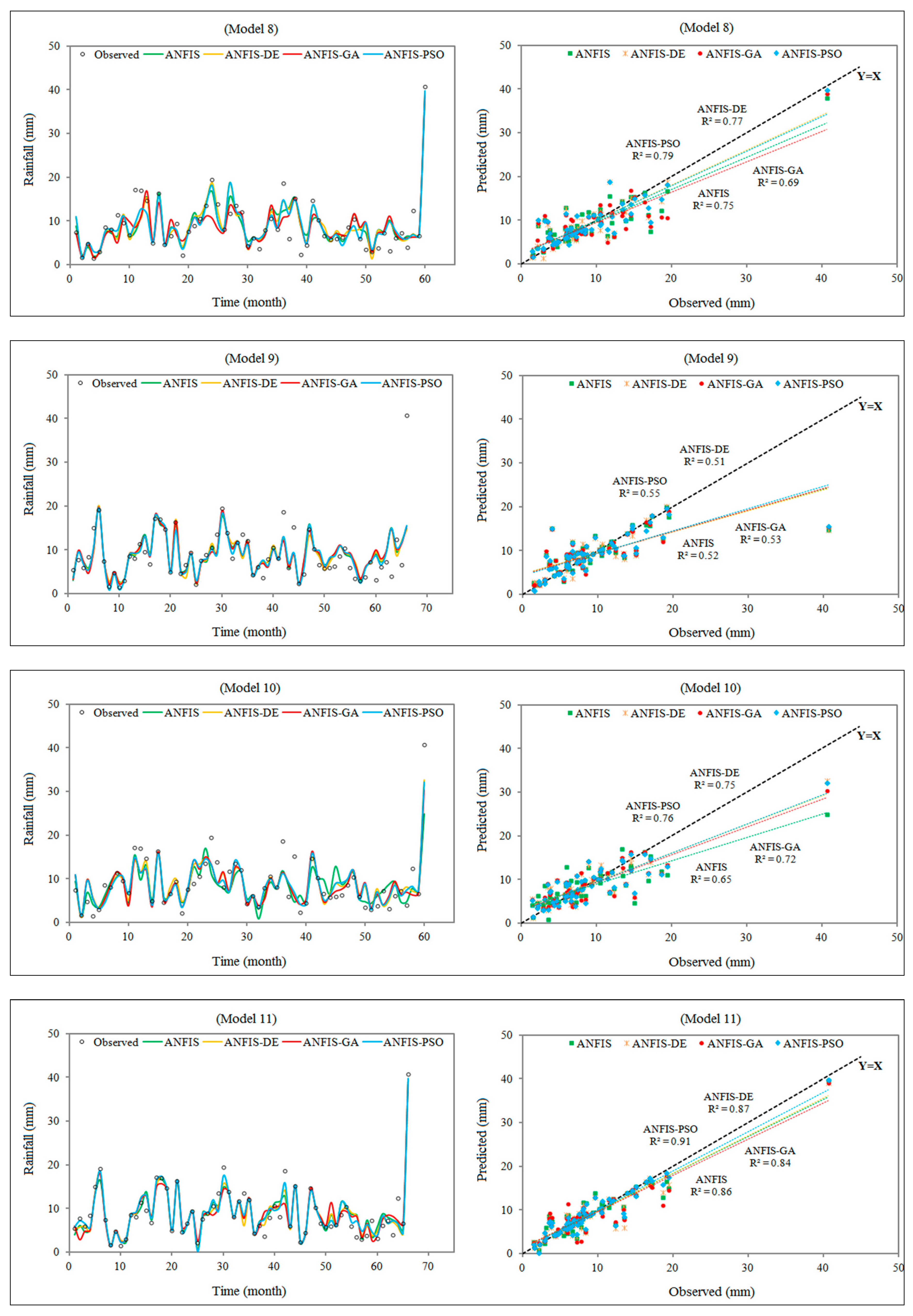
| Model 8 | 3.05 | 2.07 | 0.793 | 0.871 | 3.03 | 2.13 | 0.866 | 0.922 |
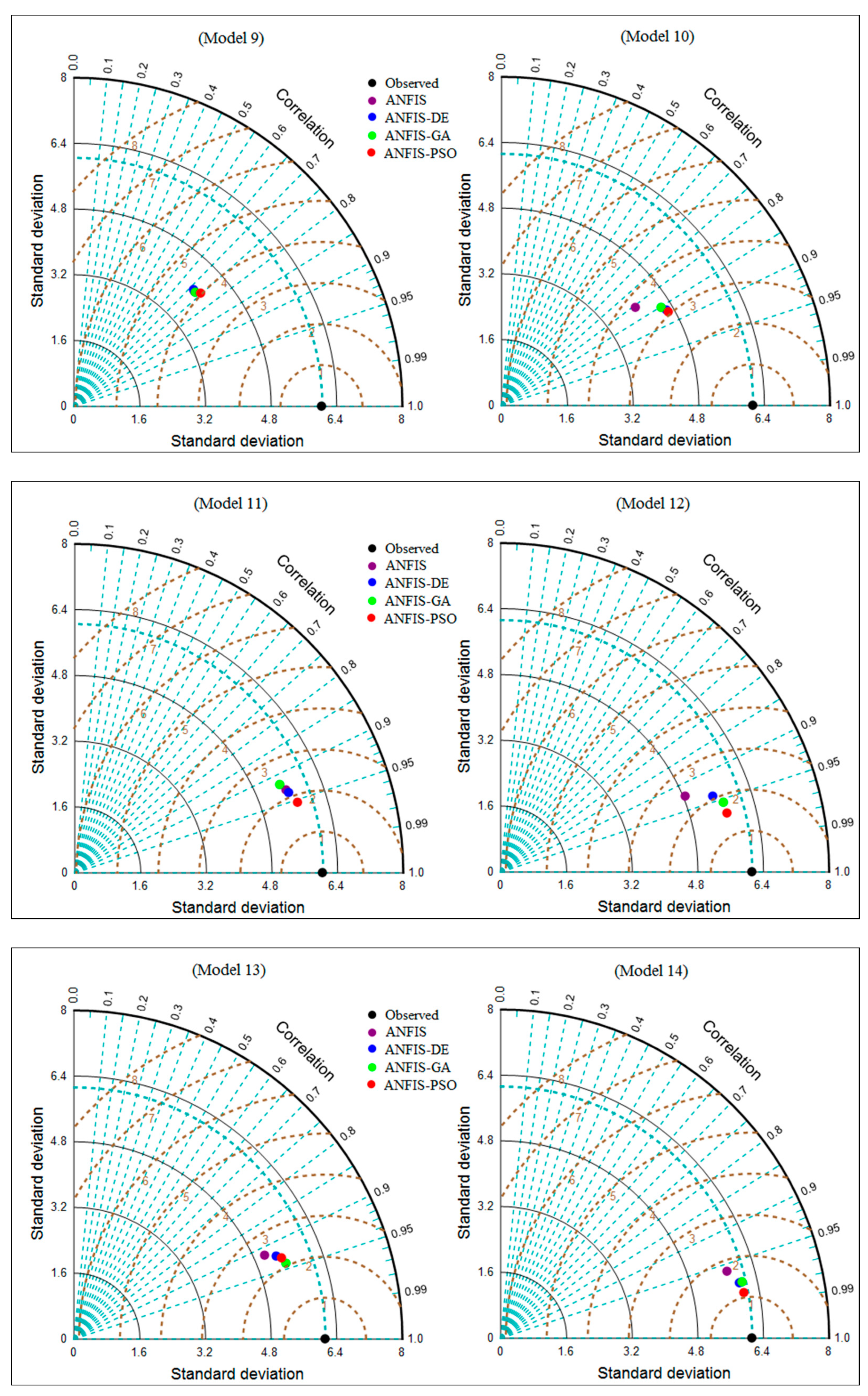
| Model 9 | 3.20 | 2.13 | 0.760 | 0.850 | 4.16 | 2.14 | 0.723 | 0.801 |
| Model 10 | 3.06 | 2.20 | 0.796 | 0.880 | 3.72 | 2.42 | 0.807 | 0.850 |
| Model 11 | 2.18 | 1.50 | 0.896 | 0.941 | 2.20 | 1.49 | 0.930 | 0.962 |
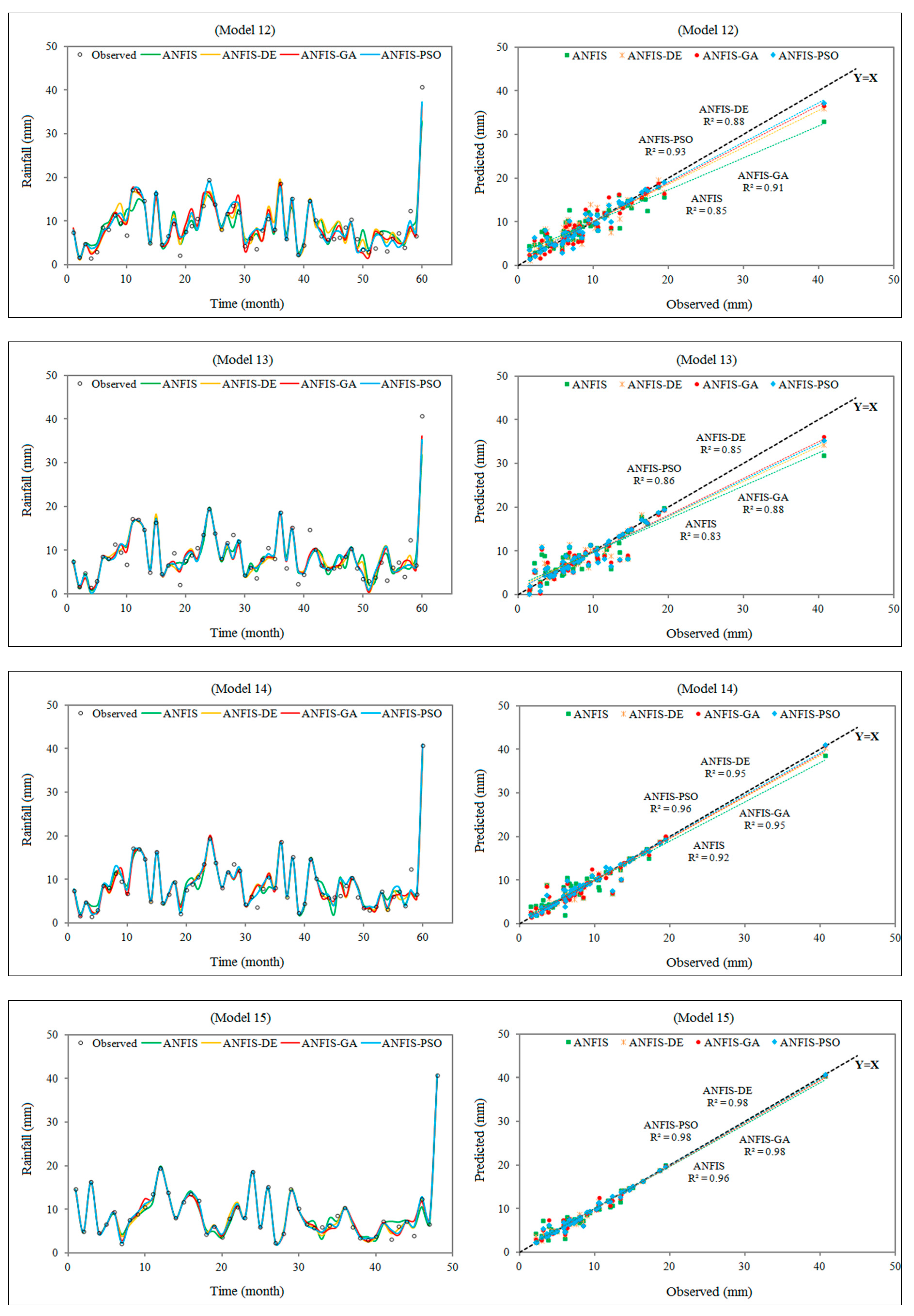
| Model 12 | 2.73 | 1.83 | 0.842 | 0.911 | 2.46 | 1.87 | 0.924 | 0.947 |
| Model 13 | 2.78 | 1.94 | 0.832 | 0.903 | 2.51 | 1.66 | 0.915 | 0.946 |
| Model 14 | 1.92 | 1.20 | 0.923 | 0.960 | 1.73 | 1.12 | 0.960 | 0.978 |
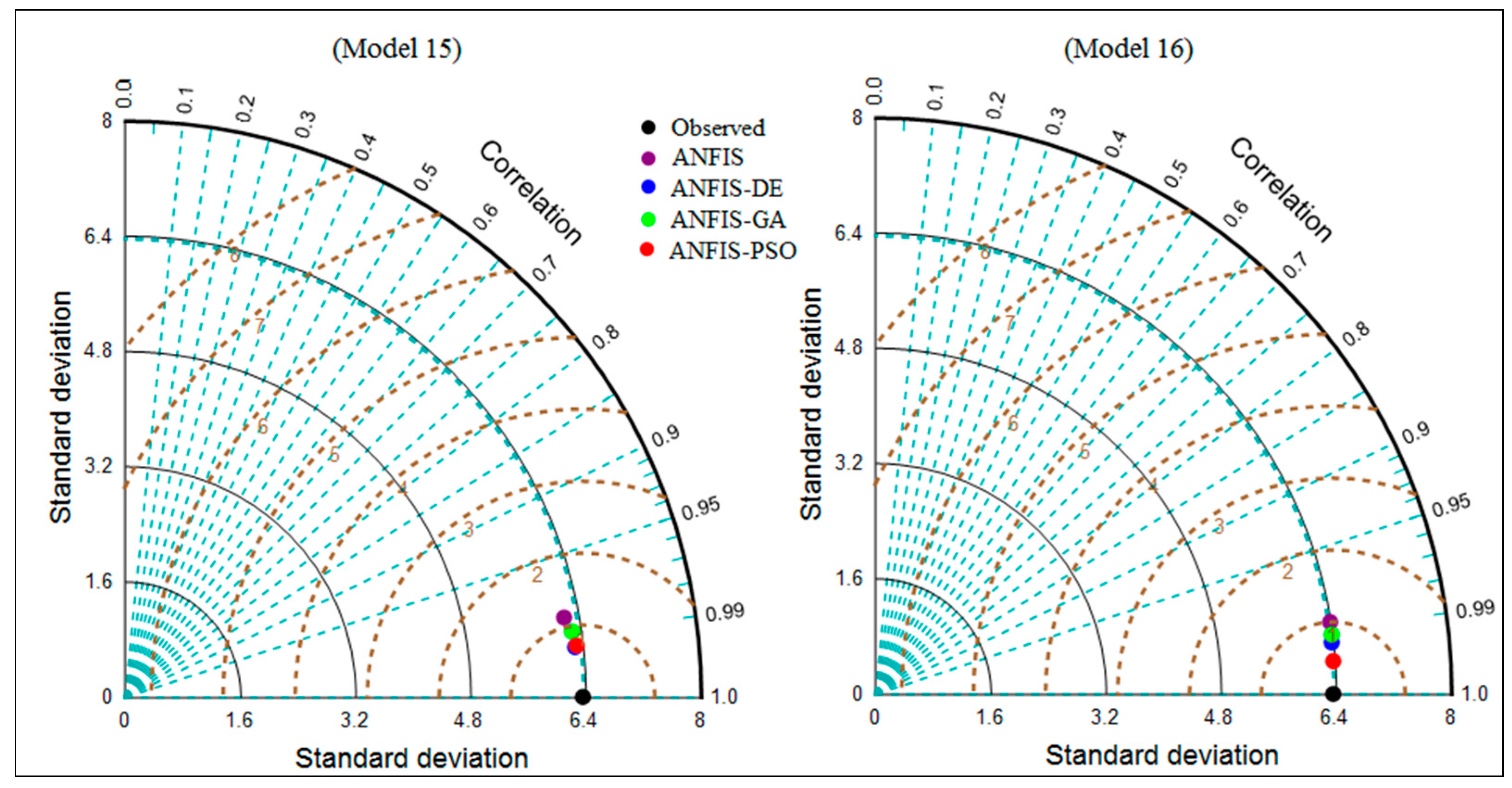
| Model 15 | 2.10 | 1.36 | 0.897 | 0.943 | 1.13 | 0.75 | 0.984 | 0.991 |
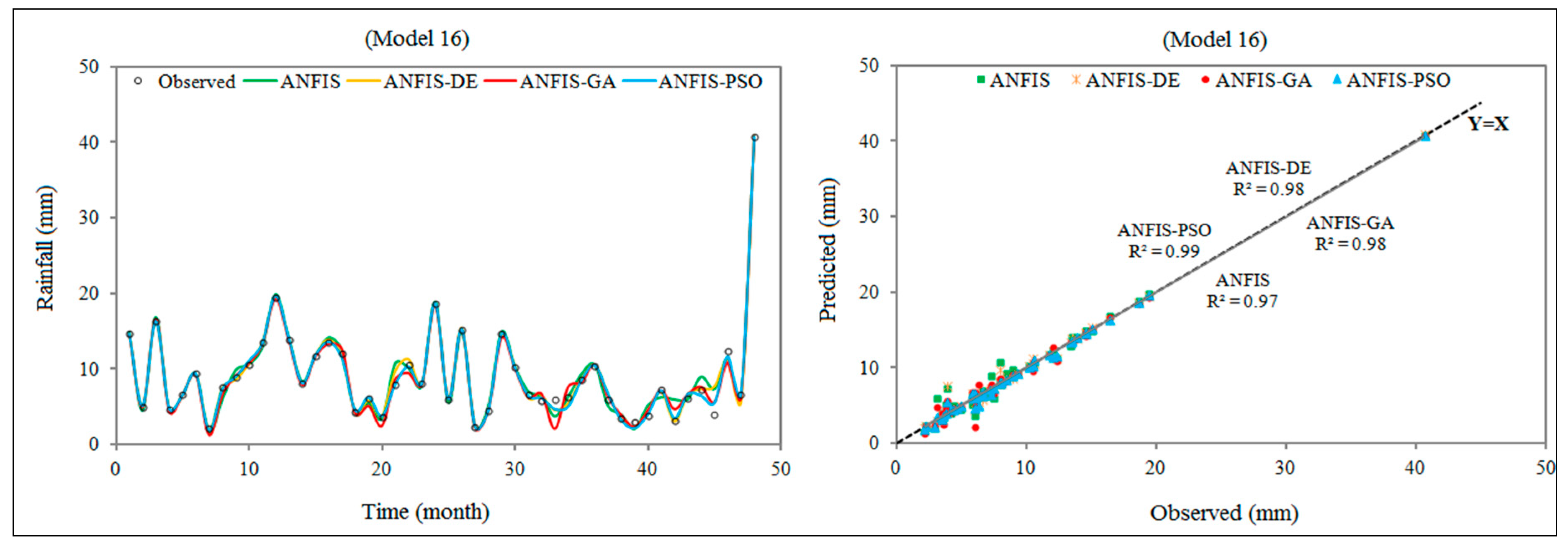
| Model 16 | 1.40 | 0.91 | 0.956 | 0.976 | 0.99 | 0.65 | 0.987 | 0.994 |
| (b) ANFIS-PSO | ||||||||
| Models | RMSE (mm) | MAE (mm) | CC | WI | RMSE (mm) | MAE (mm) | CC | WI |
| Training phase | Testing phase | |||||||
| Model 1 | 4.24 | 3.17 | 0.488 | 0.561 | 5.31 | 3.67 | 0.444 | 0.483 |
| Model 2 | 3.63 | 2.66 | 0.671 | 0.782 | 4.31 | 2.92 | 0.692 | 0.756 |
| Model 3 | 2.66 | 1.93 | 0.841 | 0.908 | 2.63 | 2.02 | 0.895 | 0.939 |
| Model 4 | 3.25 | 2.31 | 0.751 | 0.840 | 4.46 | 2.69 | 0.671 | 0.755 |
| Model 5 | 2.76 | 1.95 | 0.835 | 0.898 | 4.40 | 2.74 | 0.689 | 0.786 |
| Model 6 | 2.84 | 1.96 | 0.816 | 0.888 | 2.21 | 1.53 | 0.927 | 0.960 |
| Model 7 | 3.32 | 2.33 | 0.740 | 0.835 | 2.67 | 1.92 | 0.898 | 0.937 |
| Model 8 | 2.68 | 1.75 | 0.846 | 0.907 | 2.75 | 1.81 | 0.892 | 0.939 |
| Model 9 | 3.11 | 2.13 | 0.775 | 0.861 | 4.02 | 2.05 | 0.745 | 0.819 |
| Model 10 | 2.53 | 1.67 | 0.864 | 0.924 | 3.07 | 2.18 | 0.871 | 0.912 |
| Model 11 | 2.04 | 1.33 | 0.910 | 0.950 | 1.81 | 1.20 | 0.953 | 0.975 |
| Model 12 | 1.77 | 1.20 | 0.936 | 0.965 | 1.58 | 1.11 | 0.967 | 0.981 |
| Model 13 | 2.30 | 1.53 | 0.891 | 0.940 | 2.24 | 1.36 | 0.931 | 0.961 |
| Model 14 | 1.16 | 0.75 | 0.973 | 0.985 | 1.14 | 0.62 | 0.982 | 0.991 |
| Model 15 | 1.44 | 0.83 | 0.953 | 0.975 | 0.73 | 0.44 | 0.993 | 0.996 |
| Model 16 | 0.86 | 0.51 | 0.984 | 0.991 | 0.47 | 0.28 | 0.997 | 0.998 |
| (c) ANFIS-GA | ||||||||
| Models | RMSE (mm) | MAE (mm) | CC | WI | RMSE (mm) | MAE (mm) | CC | WI |
| Training phase | Testing phase | |||||||
| Model 1 | 4.24 | 3.17 | 0.488 | 0.561 | 5.31 | 3.67 | 0.442 | 0.481 |
| Model 2 | 3.59 | 2.62 | 0.679 | 0.791 | 4.28 | 2.85 | 0.697 | 0.758 |
| Model 3 | 2.91 | 2.10 | 0.805 | 0.881 | 2.84 | 2.28 | 0.876 | 0.928 |
| Model 4 | 3.43 | 2.37 | 0.720 | 0.822 | 4.12 | 2.47 | 0.738 | 0.794 |
| Model 5 | 2.60 | 1.78 | 0.856 | 0.911 | 3.55 | 2.28 | 0.812 | 0.890 |
| Model 6 | 2.77 | 2.02 | 0.826 | 0.895 | 2.40 | 1.72 | 0.915 | 0.951 |
| Model 7 | 3.42 | 2.15 | 0.718 | 0.812 | 2.98 | 2.02 | 0.868 | 0.922 |
| Model 8 | 2.90 | 2.01 | 0.816 | 0.884 | 3.36 | 2.28 | 0.833 | 0.900 |
| Model 9 | 3.11 | 2.07 | 0.774 | 0.860 | 4.12 | 2.12 | 0.728 | 0.806 |
| Model 10 | 2.50 | 1.63 | 0.872 | 0.930 | 3.26 | 2.27 | 0.851 | 0.898 |
| Model 11 | 2.37 | 1.60 | 0.876 | 0.930 | 2.40 | 1.53 | 0.917 | 0.954 |
| Model 12 | 2.33 | 1.59 | 0.885 | 0.935 | 1.83 | 1.35 | 0.954 | 0.975 |
| Model 13 | 2.40 | 1.57 | 0.880 | 0.932 | 2.06 | 1.30 | 0.942 | 0.967 |
| Model 14 | 1.50 | 0.93 | 0.956 | 0.976 | 1.38 | 0.78 | 0.974 | 0.986 |
| Model 15 | 1.55 | 0.92 | 0.945 | 0.970 | 0.92 | 0.56 | 0.989 | 0.994 |
| Model 16 | 1.21 | 0.69 | 0.967 | 0.982 | 0.83 | 0.51 | 0.991 | 0.995 |
| (d) ANFIS-DE | ||||||||
| Models | RMSE (mm) | MAE (mm) | CC | WI | RMSE (mm) | MAE (mm) | CC | WI |
| Training phase | Testing phase | |||||||
| Model 1 | 4.17 | 3.20 | 0.513 | 0.600 | 5.29 | 3.60 | 0.449 | 0.486 |
| Model 2 | 3.66 | 2.61 | 0.666 | 0.781 | 4.07 | 2.61 | 0.736 | 0.791 |
| Model 3 | 2.71 | 2.00 | 0.834 | 0.900 | 2.75 | 2.17 | 0.885 | 0.935 |
| Model 4 | 3.42 | 2.41 | 0.720 | 0.819 | 4.05 | 2.61 | 0.741 | 0.813 |
| Model 5 | 2.62 | 1.86 | 0.853 | 0.913 | 2.73 | 2.03 | 0.894 | 0.940 |
| Model 6 | 2.74 | 1.89 | 0.830 | 0.895 | 2.35 | 1.66 | 0.917 | 0.955 |
| Model 7 | 3.32 | 2.09 | 0.740 | 0.824 | 3.04 | 2.07 | 0.862 | 0.919 |
| Model 8 | 2.85 | 1.91 | 0.824 | 0.889 | 2.88 | 1.96 | 0.881 | 0.934 |
| Model 9 | 3.17 | 2.18 | 0.763 | 0.850 | 4.20 | 2.16 | 0.715 | 0.797 |
| Model 10 | 2.51 | 1.70 | 0.867 | 0.930 | 3.12 | 2.23 | 0.865 | 0.908 |
| Model 11 | 2.22 | 1.42 | 0.893 | 0.940 | 2.12 | 1.40 | 0.936 | 0.965 |
| Model 12 | 2.43 | 1.68 | 0.875 | 0.930 | 2.09 | 1.65 | 0.941 | 0.966 |
| Model 13 | 2.50 | 1.68 | 0.866 | 0.923 | 2.32 | 1.51 | 0.925 | 0.956 |
| Model 14 | 1.36 | 0.92 | 0.963 | 0.980 | 1.37 | 0.76 | 0.974 | 0.987 |
| Model 15 | 1.58 | 0.99 | 0.943 | 0.970 | 0.70 | 0.46 | 0.994 | 0.997 |
| Model 16 | 1.14 | 0.67 | 0.971 | 0.985 | 0.73 | 0.38 | 0.993 | 0.996 |
| Indicators | Models | ANFIS-PSO | ANFIS-GA | ANFIS-DE | ANFIS |
|---|---|---|---|---|---|
| d-factor | Model 1 | 0.14 | 0.14 | 0.14 | 0.15 |
| Model 2 | 0.68 | 0.69 | 0.69 | 0.72 | |
| Model 3 | 0.68 | 0.67 | 0.67 | 0.65 | |
| Model 4 | 0.69 | 0.69 | 0.68 | 0.67 | |
| Model 5 | 0.67 | 0.65 | 0.65 | 0.61 | |
| Model 6 | 1.17 | 1.18 | 1.18 | 1.19 | |
| Model 7 | 0.95 | 0.96 | 0.96 | 0.98 | |
| Model 8 | 1.02 | 1.02 | 1.02 | 1.03 | |
| Model 9 | 0.99 | 0.99 | 0.99 | 0.98 | |
| Model 10 | 0.88 | 0.88 | 0.88 | 0.88 | |
| Model 11 | 1.28 | 1.28 | 1.29 | 1.30 | |
| Model 12 | 1.30 | 1.31 | 1.31 | 1.32 | |
| Model 13 | 1.29 | 1.29 | 1.30 | 1.31 | |
| Model 14 | 1.43 | 1.43 | 1.44 | 1.44 | |
| Model 15 | 1.38 | 1.39 | 1.40 | 1.42 | |
| Model 16 | 1.41 | 1.41 | 1.42 | 1.43 | |
| 95PPU | Model 1 | 12.29 | 12.29 | 12.29 | 12.29 |
| Model 2 | 60.67 | 60.67 | 60.11 | 60.67 | |
| Model 3 | 57.63 | 56.50 | 55.37 | 50.28 | |
| Model 4 | 58.62 | 58.05 | 57.47 | 55.75 | |
| Model 5 | 65.48 | 64.88 | 64.29 | 61.31 | |
| Model 6 | 76.84 | 76.84 | 76.84 | 75.71 | |
| Model 7 | 66.67 | 67.24 | 64.94 | 65.52 | |
| Model 8 | 76.19 | 75.60 | 74.40 | 72.62 | |
| Model 9 | 70.11 | 69.54 | 68.39 | 65.52 | |
| Model 10 | 73.81 | 73.21 | 72.02 | 70.83 | |
| Model 11 | 79.31 | 78.74 | 78.16 | 77.59 | |
| Model 12 | 85.71 | 85.71 | 85.12 | 85.12 | |
| Model 13 | 82.74 | 82.14 | 81.55 | 81.55 | |
| Model 14 | 85.12 | 84.52 | 84.52 | 83.33 | |
| Model 15 | 89.10 | 89.10 | 88.46 | 85.26 | |
| Model 16 | 91.67 | 91.03 | 89.74 | 88.46 |
© 2019 by the authors. Licensee MDPI, Basel, Switzerland. This article is an open access article distributed under the terms and conditions of the Creative Commons Attribution (CC BY) license (http://creativecommons.org/licenses/by/4.0/).
Share and Cite
Yaseen, Z.M.; Ebtehaj, I.; Kim, S.; Sanikhani, H.; Asadi, H.; Ghareb, M.I.; Bonakdari, H.; Wan Mohtar, W.H.M.; Al-Ansari, N.; Shahid, S. Novel Hybrid Data-Intelligence Model for Forecasting Monthly Rainfall with Uncertainty Analysis. Water 2019, 11, 502. https://doi.org/10.3390/w11030502
Yaseen ZM, Ebtehaj I, Kim S, Sanikhani H, Asadi H, Ghareb MI, Bonakdari H, Wan Mohtar WHM, Al-Ansari N, Shahid S. Novel Hybrid Data-Intelligence Model for Forecasting Monthly Rainfall with Uncertainty Analysis. Water. 2019; 11(3):502. https://doi.org/10.3390/w11030502
Chicago/Turabian StyleYaseen, Zaher Mundher, Isa Ebtehaj, Sungwon Kim, Hadi Sanikhani, H. Asadi, Mazen Ismaeel Ghareb, Hossein Bonakdari, Wan Hanna Melini Wan Mohtar, Nadhir Al-Ansari, and Shamsuddin Shahid. 2019. "Novel Hybrid Data-Intelligence Model for Forecasting Monthly Rainfall with Uncertainty Analysis" Water 11, no. 3: 502. https://doi.org/10.3390/w11030502