Generating Scenarios of Cross-Correlated Demands for Modelling Water Distribution Networks

Abstract

A numerical approach for generating a limited number of water demand scenarios and estimating their occurrence probabilities in a water distribution network (WDN) is proposed. This approach makes use of the demand scaling laws in order to consider the natural variability and spatial correlation of nodal consumption. The scaling laws are employed to determine the statistics of nodal consumption as a function of the number of users and the main statistical features of the unitary user’s demand. Besides, consumption at each node is considered to follow a Gamma probability distribution. A high number of groups of cross-correlated demands, i.e., scenarios, for the entire network were generated using Latin hypercube sampling (LHS) and the numerical procedure proposed by Iman and Conover. The Kantorovich distance is used to reduce the number of scenarios and estimate their corresponding probabilities, while keeping the statistical information on nodal consumptions. By hydraulic simulation, the whole number of generated demand scenarios was used to obtain a corresponding number of pressure scenarios on which the same reduction procedure was applied. The probabilities of the reduced scenarios of pressure were compared with the corresponding probabilities of demand.

1. Introduction

The conventional modelling of water distribution networks (WDNs) is normally based on a deterministic approach, not merely with regard to the geometrical and hydraulic features, but also with respect to the demand loadings [1]. However, water demand, being influenced by many factors, i.e., type of users, socio-economic conditions, geographic location with its climate, seasonal fluctuation of weather, water fixtures technology, policies in water management, and tariffs, is subject to a natural variability. Surely, the variability of the demand represents the major source of uncertainty, which affects the overall reliability of the model for the assessment of the spatial and temporal distribution of pressure heads as well as for the evaluation of the water quality in the different pipes. Uncertainty produced by the random nature of demand assumes a different importance in relation to the spatial and temporal scales that are considered in modelling the network. Obviously, they become more and more relevant as the finer scales are reached, that is small groups of users and instantaneous demands are considered. As stated by Bargiela & Sterling [2], it is possible to obtain accurate predictions for the network as a whole, however estimating nodal consumptions for nodes where the population is low is more difficult.

Thus, considering and quantifying the uncertainty of water demand could allow for the association of an acceptable probability/level of risk to the results from hydraulic and optimization models of WDNs at different temporal and spatial scales: a more robust design and control of these systems can be realized, and obvious opportunities can arise in dimensioning pipes, formulating water balances, controlling a system’s components, and identifying and quantifying leakages.

An approach to dealing with the uncertainty of demand consists in explicitly considering different possible realizations of its value at the nodes of a WDN, i.e., different loading scenarios and associating to each of them a measure of their probability. So, it is possible to find a feasible solution which is also as close as possible to the optimum for all the scenarios: this scenario-based approach is known as robust optimization [3]. In the same way it is possible also to derive WDN reliability [4] or to localize leakages [5] or to map pressure-heads for a real-time control [6], all under uncertain demand conditions. Different possible scenarios, which include various aspects, such as peak flows, fire conditions at certain nodes, or pipe breakage, and the corresponding probabilities of occurrence could be obtained by consulting a panel of experts. However, this solution can have strong limitations in such a mathematically sensitive problem and can lead to arbitrary solutions.

To this aim, this paper focuses on defining an objective methodology for the generation of demand scenarios. In the literature, the issue of generating demand scenarios has been faced in [7] where uncertain future water consumptions are modeled using probability density functions (PDF) assigned in the problem formulation phase. Scenarios with correlated nodal demands are generated using LHS and the procedure suggested by Iman and Conover [8]. All nodal demands follow a Gaussian PDF with a coefficient of variation Cv = 0.10. The correlation coefficient between any two nodal demands is assumed equal to 0.50, as completed by Tolson et al. [9]. In [10] different demand scenarios for a WDN are derived combining demand values with a specific return period at each node. The probability of each scenario is obtained considering a multivariate normal distribution (MVN). The correlation between demand was found to significantly affect the occurrence probability of the demand scenarios. Also, Eck et al. [11] generated demand scenarios considering a MVN distribution. They assumed a prior estimate of the mean values and covariance matrix of water demand from a preliminary analysis. An original, but computationally expensive, approach for estimating the probability of a given demand scenario is based on the use of the contingency tables [12]. This is a non-parametric method in which the various random variables are divided into classes and their marginal probabilities are calculated through the frequency of occurrence of each class. The joint probabilities are evaluated by counting the occurrences of the simultaneous classes.

In this paper a numerical approach for generating a limited number of water demand scenarios and estimating their occurrence probabilities in a WDN is presented. Scaling laws [1,13,14] are used to evaluate the statistics of aggregated demand at each node of the network, starting from the statistics of demand of the unitary user. The Apulian WDN [15] is considered as a case-study and two different hypotheses are made for the number of users in the nodes. For each of these hypotheses a large number of cross-correlated demands, i.e., scenarios, was generated using LHS from Gamma PDF and a procedure based on the approach proposed by Iman and Conover [8]. The Kantorovich distance [16] is used to reduce the number of scenarios and estimate their corresponding probabilities. In this way, the limited number of network demand scenarios maintain the statistical information on the demand and the effects on the performance of a WDN. In the design and control of WDNs, demand scenarios are mostly functional to the evaluation of service conditions and specifically pressure-heads in the nodes. In order to evaluate how the uncertainty of demand is conveyed to the pressure-head field, a demand-driven hydraulic model was also applied to solve the Apulian network. Many pressure scenarios were obtained, and the same reduction procedure was employed. The probabilities of the reduced scenarios of pressure were compared with the corresponding probabilities of the demand.

Here, a brief summary of the structure of this work is presented. In Section 2 the description of the proposed methodology is provided. In particular, a summary of the scaling law approach for water demand is reported in Section 2.1, the scenario generation procedure in Section 2.2, and the scenario reduction procedure in Section 2.3. In Section 3 an example is carried out by applying the whole procedure on a literature WDN and the results are discussed. Finally, Section 4 provides some conclusive comments.

2. Description of Methodology

2.1. Scaling Laws

In the first phase of the proposed methodology, the statistical features of WDN nodal demand are derived using the scaling laws [1,13]: i.e., the first and second statistical moments and cross-correlation are evaluated, and the probability distributions defined. Input data are the nodal number of consumers and the statistical features of water demand of the typical single user, the unitary user. The statistical parameters of the unitary user’s demand can be derived either by monitoring, or simulating by descriptive models, such as End-Uses models [17] or Poisson Rectangular Pulse models preserving correlation [18].

We consider a network with $i=1,2,3,\dots ,N$ nodes and $n_i=n_1,n_2,n_3,\dots ,n_N$ users at each node. The demand of a unitary user, identified by subscript 1, is described by an ergodic stationary stochastic process, with mean ${\mu }_1$, variance ${\sigma }_1^2$ and cross-correlation coefficient between each couple of single-user ${\rho }_1$. The whole nodal demand, that is the sum of all users’ consumption at each node, is a realization of the stochastic process whose statistics are dependent on the number of nodal users. The expected value $E[{\mu }_{n_i}]$ for the mean of the aggregated process at the ith node is given by:

$$E[{\mu }_{n_i}]=n_i·E[{\mu }_i],$$

(1)

and the expected value for the variance $E[{\sigma }_{n_i}^2]$ at the same node, neglecting the bias that can be caused when using small the demand series (short observation periods) [13], is given by:

$$E[{\sigma }_{n_i}^2]=n_i{}^2·E[{\rho }_1]·E[{\sigma }_1^2]+n_i·[1-\mathrm{E}[{\rho }_1]]·E[{\sigma }_1^2]$$

(2)

Equation (2) shows that the expected value of the variance of the aggregated process depends on $\mathrm{E}[{\rho }_1]:$ if demands are perfectly correlated in space, i.e., $E[{\rho }_1]$ is equal to one, Equation (2) is simplified into:

$$E[{\sigma }_{n_i}^2]=n_i{}^2·E[{\sigma }_1^2]$$

(2a)

if demands are uncorrelated in space, i.e., $E[{\rho }_1]$ is equal to zero, equation [2] is simplified into:

$$E[{\sigma }_{n_i}^2]=n_i·E[{\sigma }_1^2]$$

(2b)

For partially correlated demands, a power law $E[{\sigma }_{n_i}^2]=n_i^{\alpha }E[{\sigma }_1^2]$, with α scaling variance exponent, has been also derived [1,14]. Therefore, a complete statistical characterization of demand requires not only the definition of its mean and variance, but also the definition of the correlation between demands of each couplet of users and groups of users. The cross-correlation refers to the similarity between demand patterns from different consumers or from different nodes. This parameter was proved to be not negligible [19] and to affect the hydraulic performance of a WDN as well as the cost to achieve a desired level of reliability. It was verified that higher cross correlations lead to higher pressure fluctuations, which have negative impacts on the reliability of the WDN [20]. Following the same assumption and notation, the expected value for the cross-correlation between all nodes of the network is represented by a N-by-N square matrix, whose elements are given by:

$$E\left[{\rho }_{n_i{n}_j}\right]=\frac{E\left[co{v}_{n_i{n}_j}\right]}{E\left[{\sigma }_{n_i}\right]·E\left[{\sigma }_{n_j}\right]}=\frac{n_i{n}_{j}E\left[{\rho }_1\right]}{{[n_i\left(1+E[{\rho }_1]\left(n_i-1\right)\right)]}^{\raisebox{1ex}{$1$}\!\left/ \!\raisebox{-1ex}{$2$}\right.}·{[n_j\left(1+E[{\rho }_1]\left(n_j-1\right)\right)]}^{\raisebox{1ex}{$1$}\!\left/ \!\raisebox{-1ex}{$2$}\right.}}$$

(3)

with $i,j=1,2,3,\dots ,N$, and where, for example, ${\rho }_{n_1{n}_2}$ is the cross-correlation coefficient between the demand of $n_1$ aggregated users at node 1, and the demand of $n_2$ aggregated users at node 2.

Through Equations (1)–(3) the nodal demand statistics of the network and the correlation structure between them are entirely defined.

2.2. Generation of Scenarios

In simulation and optimization problems, several methods exist to cope with uncertainty [21,22]. If we do not know exactly the input data, in our case water demand at the nodes of a WDN, because they can assume different values and then many combinations of them are possible, we are dealing with scenarios. But, if the statistical features of uncertain data are known, numerical solutions can be obtained by approximating the probability distribution function with discrete distributions having a finite number of outputs, again referred to as scenarios.

Then, the second phase of the present approach consists in the generation of a large number of water demand scenarios for a WDN, based on the statistics estimated by the scaling laws and making the hypothesis of Gamma-distributed water demand at each node. The knowledge of the scaling laws of the statistical moments and the type of the probability distributions of water demand in relation to the number of users, prove to be a useful tool to face the inherent uncertainty of demand and in particular to address the optimization problems. Using Gamma distribution for demand is supported when the number of aggregated users is high enough or the time resolution is greater than five minutes, by measurements in the Latina case-study [1]. Furthermore, in a recent work Kossieris and Makropoulos [23] investigated the performance of ten probabilistic models showing that both Gamma and Weibull distributions can be used to adequately describe the nonzero water demand recorded at different time scales.

Scenarios can be generated following different methods: by matching a small set of statistical properties, e.g., moments [24,25] or simulating some defined mathematical process (e.g., Brownian motion) or sampling from known distributions [26]. For scenarios with a large number of variables correlated in between, sampling from the joint distribution is not usual for the difficulty in defining the distribution itself. An alternative to specifying the joint distribution is to make use of just the marginal distributions and the linear or rank correlation matrix alone. If nothing is known about the form of the joint distribution, a coupling procedure can be used: in this case the generated scenarios will respect an arbitrary dependency structure based on the procedure followed.

Each demand scenario $D_u$ is defined here as a set or combination of nodal demand values occurring simultaneously in the WDS. This can be represented by the N dimensional vector:

$$D_u=[d_{1,u},d_{2,u},\dots d_{N,u}],$$

(4)

where $u=1,2,\dots ,S$ is the index identifying the different scenarios, and $d_{i,u}$ is the demand at node i for the $uth$ scenario and $D_u$ depicts a one-dimensional stochastic data process.

A sampling method from the marginal distribution based on the LHS and the Iman-Conover approach [8] is followed. The restricted pairing technique by Iman and Conover induces rank correlation between the given marginals by shuffling finite-size samples from each of them. The appropriate shuffle is determined by ranking the input samples the same as in a reference sample with the desired rank correlation. The complete procedure, that will be described in the following, is quite straightforward because it requires only the Cholesky decomposition, some matrix algebra, and the final rearrangement of the original uncorrelated sample.

Description of the Procedure:

Step 1.

Create a random (S, N) dimensional matrix Z*, containing S Latin Hypercube Samples of size N from a standardized normal distribution, where S is the number of scenarios and N the number of the demand nodes in the WDN. For this purpose, the Matlab function lhsnorm was used. Owing to the finite size of the samples their correlation matrix I* (Here, the asterisk is used to distinguish data and corresponding correlation matrices to be corrected) does not coincide with the identity matrix I, that is they are not independent. Then, the lower triangular Cholesky decomposition is applied to induce the desired correlation [27]. Specifically:

$$\begin{array}{c}I=C·C^T\\ I^{*}=E·E^T\\ Z=Z^{*}·C·E^{-1}\end{array}$$

(5)

and the (S, N) dimensional matrix Z of perfectly independent S samples of size N from a standardized normal distribution is obtained. In order to obtain the Cholesky root, the Matlab function chol was used.

Step 2.

Create a random (S, N) dimensional matrix G containing S standardized normal samples with the correlation matrix Corr from the scaling laws for nodal demand. To this aim the desired correlation is induced in Z also applying the lower triangular Cholesky decomposition [27], that is:

$$Corr=P·P^{T}G=Z·P·C^{-1}$$

(6)

Step 3.

Transform the matrix G in the (S, N) dimensional matrix D* which complies with the desired marginal distributions at each demand ith node. Transformation is based on the inverse cumulative distribution function, CDF, of the desired marginals, F_i. Specifically, for each element D*_i of matrix D*, i.e., a non-normal random sample with the desired CDF, the following equation holds:

$$D_i^{*}=F_i^{-1}\left(\mathsf{\Phi }\left(G_i\right)\right)$$

(7)

where $\mathsf{\Phi }\left(G_i\right)$ is the CDF of the ith samples of G and it is uniformly distributed. This procedure is known as the inverse transformation method [28]. Function $\mathsf{\Phi }\left(G_i\right)$ can also be interpreted as a realization from the Gaussian copula. Applying the inverse CDF $F_i^{-1}$ to the uniform random variable $\mathsf{\Phi }\left(G_i\right)$ ensures that $D_i^{*}$ is distributed according to ${\mathsf{\Phi }}_i$. Unfortunately, the transformation in Equation (1) is non-linear, and therefore the correlation matrix Corr* of D* is not equal to the desired correlation matrix Corr.

Step 4.

Apply the Iman-Conover algorithm proposed by Ekström [29] in order to get a better approximation of the desired correlation matrix Corr for the (S, N) matrix of nodal demand scenarios D*. The algorithm is described in the following steps:

4.1

Calculate lower triangular Cholesky decomposition V of Corr, i.e., Corr = V∙V^T.

4.2

Calculate lower triangular Cholesky decomposition Q of Corr*, i.e., Corr* = Q∙Q^T.

4.3

Obtain T such that Corr = T∙Corr∙T^T, can be calculated as T = V∙Q⁻¹.

4.4

Obtain the matrix ScoreD* by rank-transforming D and convert to van der Waerden scores, defined as $F_i^{-1}\left(\mathsf{\Phi }\left(i/(N+1\right)\right)$ where ϕ is the CDF of the standard normal distribution, i is the assigned rank and N is the total number of samples.

4.5

Calculate the target scores matrix ScoreD = ScoreD*·T^T.

4.6

Match up the rank pairing in D* according to ScoreD, obtaining the new (S,N) dimensional matrix D containing the S scenarios of the N nodal demand in the WDS. The N samples are distributed according to the desired marginals and their correlation matrix is close to the correlation matrix derived from the scaling laws.

2.3. Scenario Reduction

With the scenario generation procedure, we obtain a great number of pictures, each of which represent a single snapshot of the whole water demand in the network. The higher the number of scenarios generated, the better the description of the variability of water demand in the WDS. However, it is not possible to manage such a large number of scenarios to deal with stochastic or robust optimization problems. Moreover, the probability associated with each of them is not very significant. We have to reduce the scenarios and at the same time determine, for the reduced scenarios, a significant weight representative of their possibility to be realized. Then, the goal of scenario reduction is to approximate the discrete distribution of the generated scenarios with another discrete distribution having fewer elements. At this point, the choice of the number of scenarios becomes a critical step in obtaining meaningful solutions taking into account the system performance and the robustness of the solution to variations in the uncertain data.

It is assumed that the probability distribution $\mathbb{P}$ of the N-dimensional stochastic data process is approximately given by many scenarios:

$$D_u=[d_{1,u},d_{2,u},\dots d_{N,u}],u=1,2,\dots ,S$$

(8)

to which the probabilities $p_u$ are associated and ${\sum }_{u=1}^S{p}_u=1$.

In order to approximate the probability distribution $\mathbb{P}$ with another $\mathbb{Q}$ distribution, with a smaller number of elements, so that $\mathbb{Q}$ will be as close as possible to $\mathbb{P}$ in terms of probabilistic distance, we use the Kantorovich distance, $K$, which is the most common probability distance used in stochastic optimization [30]. It represents the optimal value to a linear transportation problem. In this problem a cost function $c_N$, defined by some norm $\left|.\right|$ on ${\Re }^n$ is introduced as a measure of the distance between couples of scenarios [30].

The previous problem is not easy to solve and in order to overcome to these difficulties, heuristic algorithms have been developed, in particular fast-backward and fast forward strategies have been implemented [31]. In this paper, we make use of the forward selection algorithm. It defines an iterative process which starts with an empty set. At each iteration, from the set of the non-selected scenarios, the scenario minimizing the Kantorovich distance between the reduced and original sets is selected and inserted in a reduced set. The optimal selection of a single scenario may be repeated recursively until the prescribed number S of elements is reached.

Actually, the forward selection algorithm does not guarantee that the reduced set of scenarios is the closest in the Kantorovich distance with respect to the original set and represents the optimal solution of the original transportation problem. However, the empirical results described in the literature [32] indicate that the forward selection algorithm works well in practice.

Description of the Procedure:

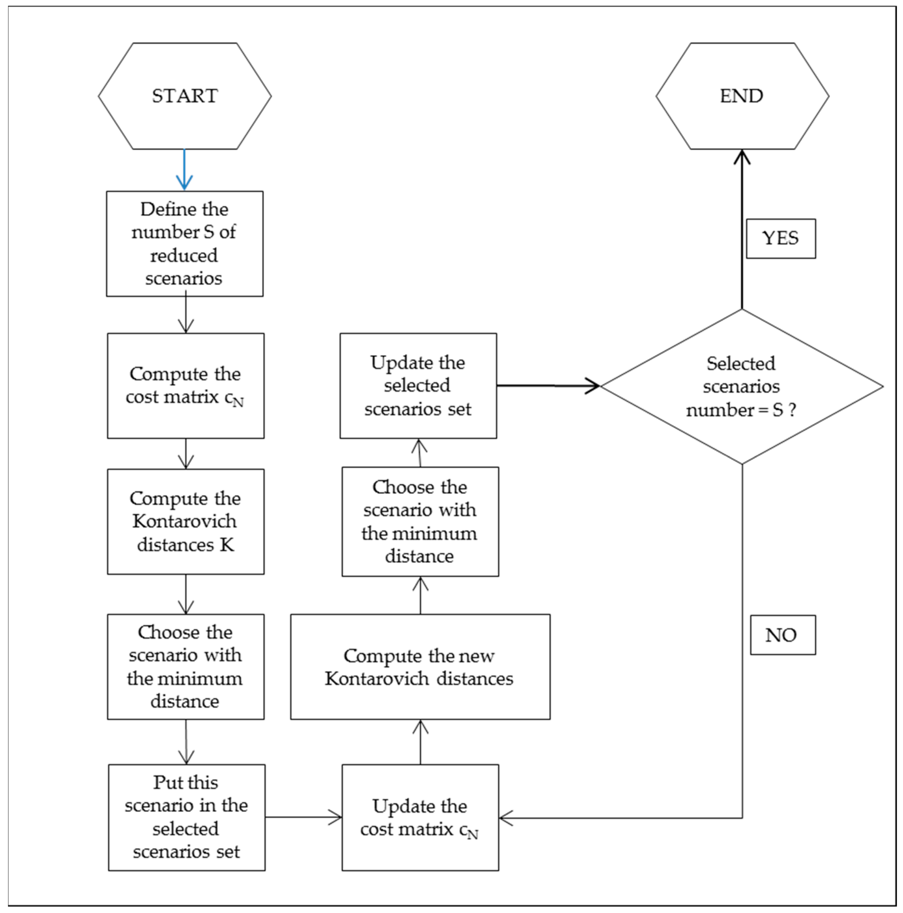
In this paper a scenario reduction algorithm based on Kantorovich distance was used (Figure 1). In particular, the fast-forward selection algorithm as described in [30] was applied. Starting from an empty set, an iterative process was followed until the required number of selected scenarios was reached. In the following is reported a brief description of this methodology.

First, the high number of generated demand scenarios at each node have been assumed to be equiprobable. Thus, at each iteration, using the Euclidean norm ${\ell }^2$, the distances between all the possible pairs of scenarios were calculated for each node. Then, by summing the corresponding distances for all the different nodes, the cost function matrix $c_N$ was derived considering the Euclidean norm. This function allows the evaluation of the Kantorovich distances matrix between pairs of scenarios taking into account their probability of occurrence.

The scenario corresponding to the minimum value of the Kantorovich distance is then selected and the cost matrix is updated by replacing each element with the minimum value between the original element and the one corresponding to the selected scenario. At this point, the procedure is repeated, and a new scenario is added to the reduced scenario set until the number of requested scenarios is reached. In the end, an optimal redistribution of probabilities was carried out by adding the probabilities of non-selected scenarios to the probabilities of those in the reduced set, that is the probability of each non-selected scenario was summed to the probability of the closest selected scenario according to the cost function.

Therefore, according to equation, the new probability of a preserved scenario is equal to the sum of its former probability and all the probabilities of the deleted scenarios that are closest to it according to $c_N$. Obviously, the deleted scenarios have probability zero.

3. Application Example

3.1. Theoretical WDN: The Apulian Network

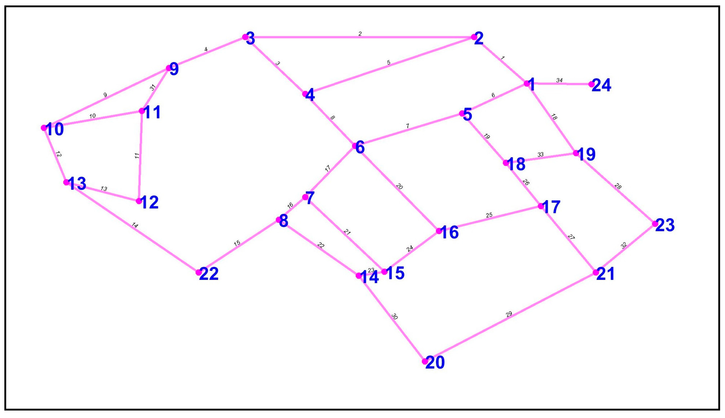
For a better understanding of the developed approach, an application using the Apulian network layout [15] is elaborated as an example. The Apulian network layout comprises 1 reservoir, 23 demand nodes and 34 pipes (Figure 2).

This network is used only with the objective of defining a scene and providing visual help to the application example. The scaling laws have an important role, mostly when the number of users at each node is low and the sampling time short, because in this case the cross-correlation between pairs of nodal demands preserves values that are not too large. In great WDN the approach can be used but it is significant only if the network is well described, i.e., it is not too skeletonized. Otherwise, with a great number of users in the nodes, the most probable scenario can be derived by simply considering the mean demand in the node. The Apulian network is representative of a real situation and its small size determines very short computational times and makes more readable the results. The geometrical features of the WDN are summarized in

Table 1. WDN geometrical features, number of users and water demand at nodes.

PIPES
Pipe Number	Start Node	End Node	Length (m)	C Hazen Williams	D (m)	Pipe Number	Start Node	End Node	Length (m)	C Hazen Williams	D (m)
1	1	2	348.5	100	0.327	18	1	19	583.9	100	0.164
2	2	3	955.7	100	0.29	19	5	18	452	100	0.229
3	3	4	483	100	0.1	20	6	16	794.7	100	0.1
4	3	9	400.7	100	0.29	21	7	15	717.7	100	0.1
5	2	4	791.9	100	0.1	22	8	14	655.6	100	0.258
6	1	5	404.4	100	0.368	23	15	14	165.5	100	0.1
7	5	6	390.6	100	0.327	24	16	15	252.1	100	0.1
8	6	4	482.3	100	0.1	25	17	16	331.5	100	0.1
9	9	10	934.4	100	0.1	26	18	17	500	100	0.204
10	11	10	431.3	100	0.184	27	17	21	579.9	100	0.164
11	11	12	513.1	100	0.1	28	19	23	842.8	100	0.1
12	10	13	428.4	100	0.184	29	21	20	792.6	100	0.1
13	12	13	419	100	0.1	30	20	14	846.3	100	0.184
14	22	13	1023.1	100	0.1	31	9	11	164	100	0.258
15	8	22	455.1	100	0.164	32	23	21	427.9	100	0.1
16	7	8	182.6	100	0.29	33	19	18	379.2	100	0.1
17	6	7	221.3	100	0.29	34	24	1	158.2	100	0.368
NODES
node ID		elevation (m)		users A		DemandA (l/s)		users B		DemandB (l/s)
1		6.4		932		10.86		155		1.8
2		7		1461		17.03		427		4.98
3		6		1282		14.95		48		0.56
4		8.4		1224		14.28		129		1.5
5		7.4		869		10.13		1270		14.81
6		9		1316		15.35		486		5.67
7		9.1		782		9.11		63		0.73
8		9.5		901		10.51		766		8.93
9		8.4		1045		12.18		63		0.73
10		10.5		1249		14.57		45		0.52
11		9.6		848		9.88		964		11.24
12		11.7		650		7.58		354		4.12
13		12.3		1303		15.2		122		1.42
14		10.6		1162		13.55		185		2.15
15		10.1		791		9.23		81		0.94
16		9.5		960		11.2		55		0.64
17		10.2		984		11.47		968		11.29
18		9.6		928		10.82		55		0.64
19		9.1		1258		14.68		45		0.52
20		13.9		1142		13.32		416		4.85
21		11.1		1255		14.63		567		6.61
22		11.4		1030		12.01		137		1.59
23		10		886		10.33		920		10.73
24 (Reservoir)		36.4		24258		282.86		8321		96.97

.

Data from two-years long water demand measurements of 82 single household users in the town of Latina, Italy [1] were considered for the definition of the statistical parameters of a typical residential consumption and the calibration of the scaling laws.

Table 2. Relevant statistics and parameters derived from the consumption data of Latina.

Statistical Parameter	Value
${\mu }_{average}\left(\mathrm{L}/\min \right)$	0.365
${\mu }_{peakhour}\left(\mathrm{L}/\min \right)$	0.700
${\sigma }_{peakhour}\left(\mathrm{L}/\min \right)$	0.870
scaling law exponent α	1.230

summarizes the average water demand of each typical user and its relevant statistics at peak hour (7:00 a.m.–8:00 a.m.), considering a five-minute time step in data monitoring. The users were considered all the same type and for this reason the same statistical parameters were employed. The number of users at each node of the WDN is also listed in Table 1. In the following examples, residential water consumers are considered, but the approach can be applied to any type of consumption, provided that the statistical characteristics of the typical user are available through monitoring or numerical simulation. Regarding the correlation between pairs of single households a very low value of the Pearson coefficient, i.e., E[ρ₁] = 0.0043, was considered, in agreement with most of the experimental data from the case study of Latina. Table 1 also shows the number of consumption units for each water demand node. In order to highlight how the number of users per node and their relationships affect the generated demand scenarios two different frameworks were examined to which correspond respectively DemandA and DemandB column. The DemandA values are the same used by Giustolisi et al. [33] for Apulian network and the users’ number is consequent. Differently, DemandB values were defined assuming a smaller total number of users and a greater variability of the number of users per node.

3.2. Generation of Demand Scenarios

The methodology presented in this work was applied to generate scenarios of contemporary water demands in the supply nodes of the Apulian distribution network. Two different hypotheses have been made on the number of users at the demand nodes. In the first one, DemandA, the number of users was determined in order to obtain the demand values assumed by Giustolisi et al. [33], which are appropriate for the subsequent hydraulic simulation of the network. Instead, the second hypothesis, DemandB, considers a lower number of total users, but, above all, considerably differentiates the number of users at each node. This was done with the aim of highlighting how the correlation matrix obtained from the scaling laws is influenced by the number of users in the nodes and by their mutual relations, and the proposed methodology can manage complex scenarios. The statistical parameters describing the unitary user’s demand are obtained from the experimental data of a group of users in the case study of Latina [1]. Data are referred to peak hour and their sampling interval is equal to five minutes.

3.2.1. DemandA

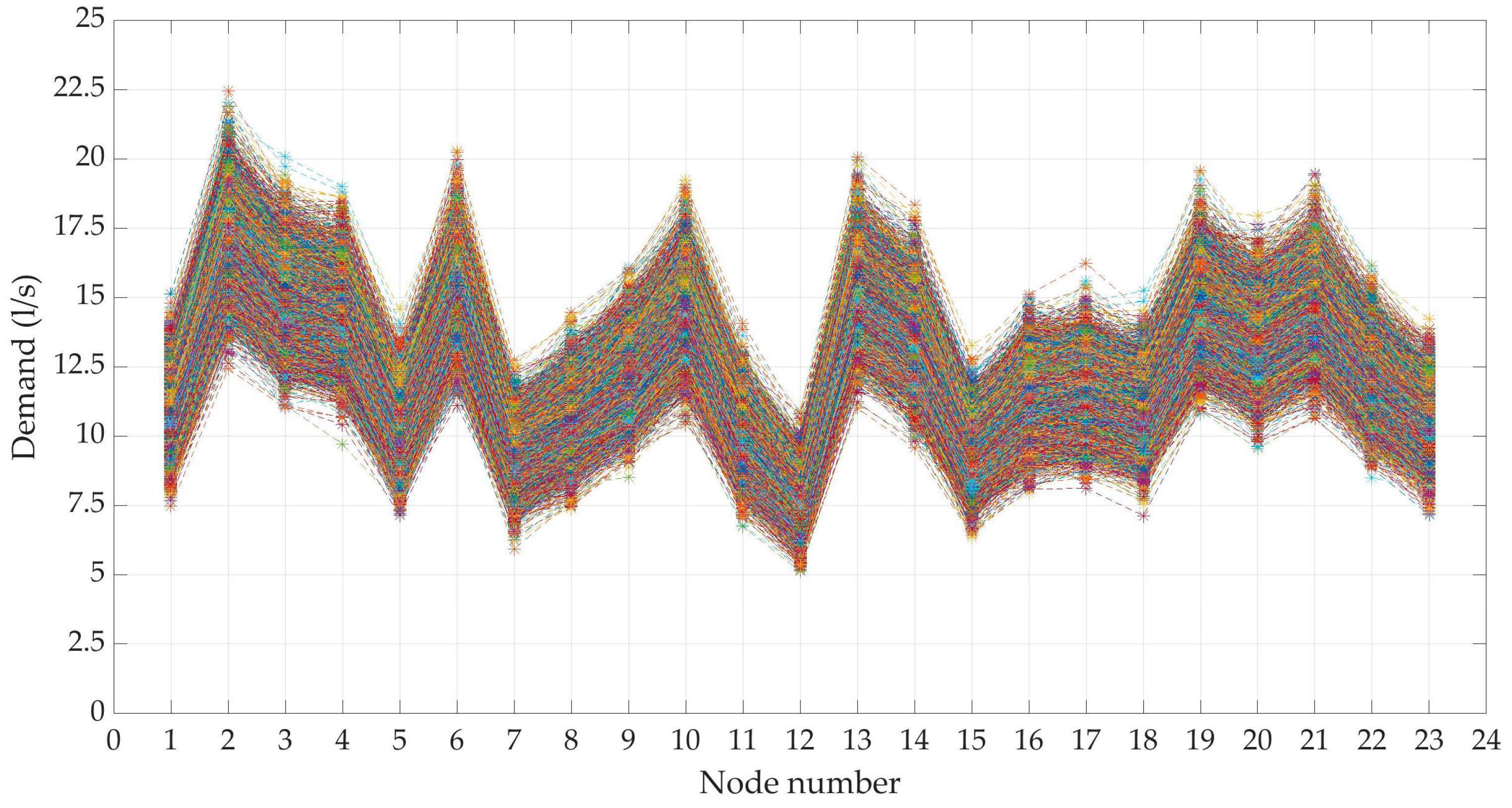
Twelve-thousand demand scenarios were generated using the statistics estimated by the scaling laws and making the hypothesis of Gamma-distribution at each node, as shown in Figure 3. The large number of scenarios makes it difficult to distinguish them. But above all, nothing can be said about their probability.

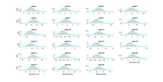
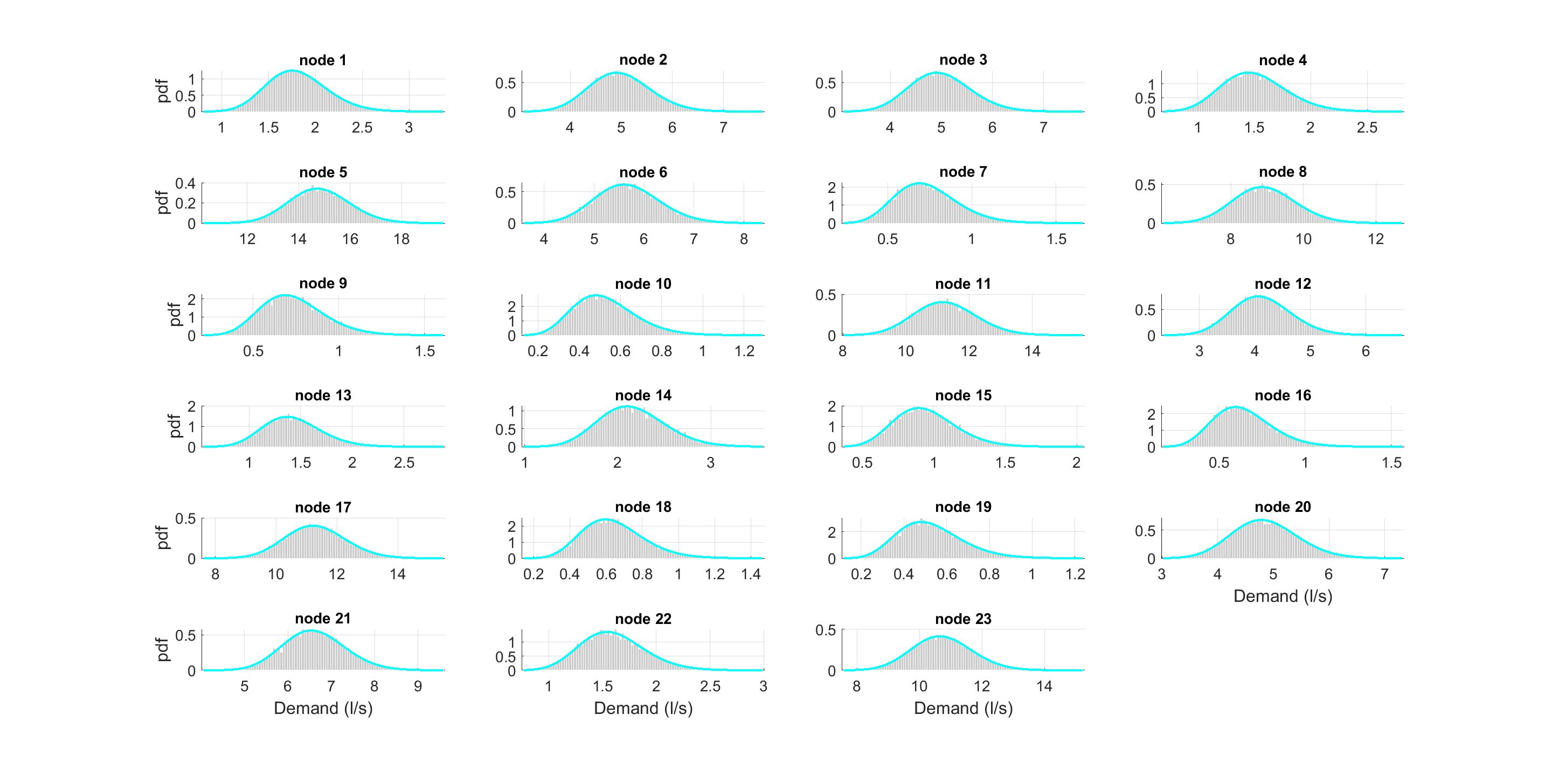
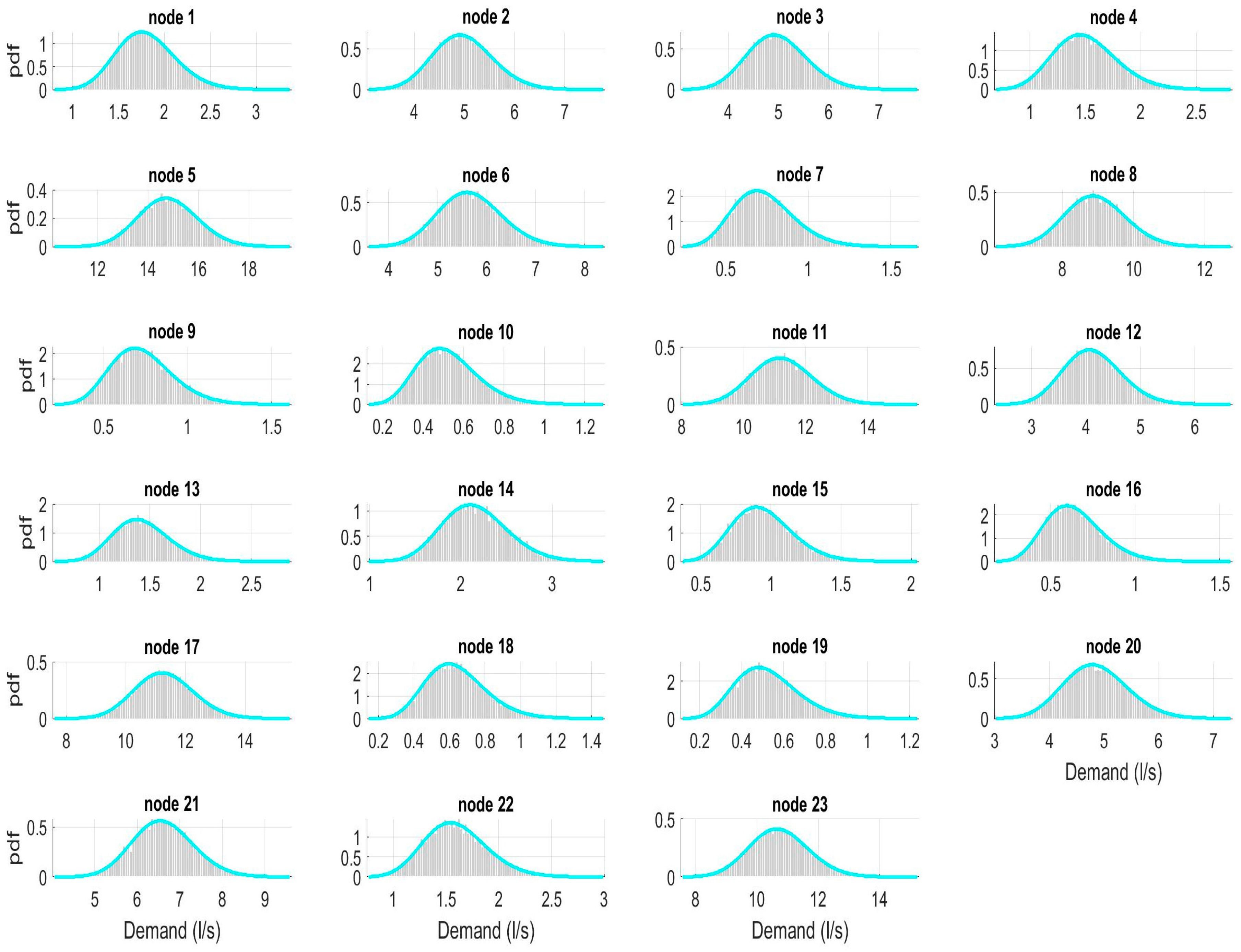
Gamma distribution proves to be the best in fitting the generated data in all nodes of the WDN, as shown in Figure 4. The scale and shape parameters of the input distributions Γ(a,b), estimated by the scaling laws (INPUT), agree well with the corresponding parameters of the generated scenarios (OUTPUT),

Table 3. Parameters a and b of Gamma distributions of input and output data, DemandA.

	INPUT		OUTPUT			INPUT		OUTPUT
Node ID	a	b	a	b	Node ID	a	b	a	b
1	125.20	0.0868	125.21	0.0868	13	162.06	0.0938	162.07	0.0938
2	176.99	0.0963	177.01	0.0963	14	148.38	0.0914	148.39	0.0914
3	160.04	0.0935	160.06	0.0934	15	110.35	0.0836	110.36	0.0836
4	154.44	0.0925	154.45	0.0925	16	128.09	0.0874	128.10	0.0874
5	118.63	0.0855	118.65	0.0855	17	130.55	0.0879	130.56	0.0879
6	163.30	0.0940	163.32	0.0940	18	124.79	0.0868	124.80	0.0868
7	109.38	0.0834	109.39	0.0834	19	157.73	0.0930	157.75	0.0930
8	121.98	0.0862	122.00	0.0862	20	146.41	0.0910	146.42	0.0910
9	136.73	0.0892	136.75	0.0892	21	157.44	0.0930	157.46	0.0930
10	156.86	0.0929	156.88	0.0929	22	135.22	0.0889	135.24	0.0889
11	116.42	0.0850	116.43	0.0850	23	120.42	0.0858	120.43	0.0858
12	94.86	0.0799	94.87	0.0799	-	-	-	-	-

. Regarding the correlation matrix of the generated scenarios, it almost perfectly matches with the input correlation matrix obtained from the scaling laws.

Table 4. Min, average, max values of input and output cross-correlation matrix, DemandA.

	E[ρ1] = 0.0043
	ρ Input Correlation Matrix (Scaling Laws)	ρ Output Correlation Matrix (Scenarios)
min	0.7542	0.7542
average	0.8147	0.8147
max	0.8568	0.8567

compares the minimum, average and maximum value of the input and output correlation matrices.

3.2.2. DemandB

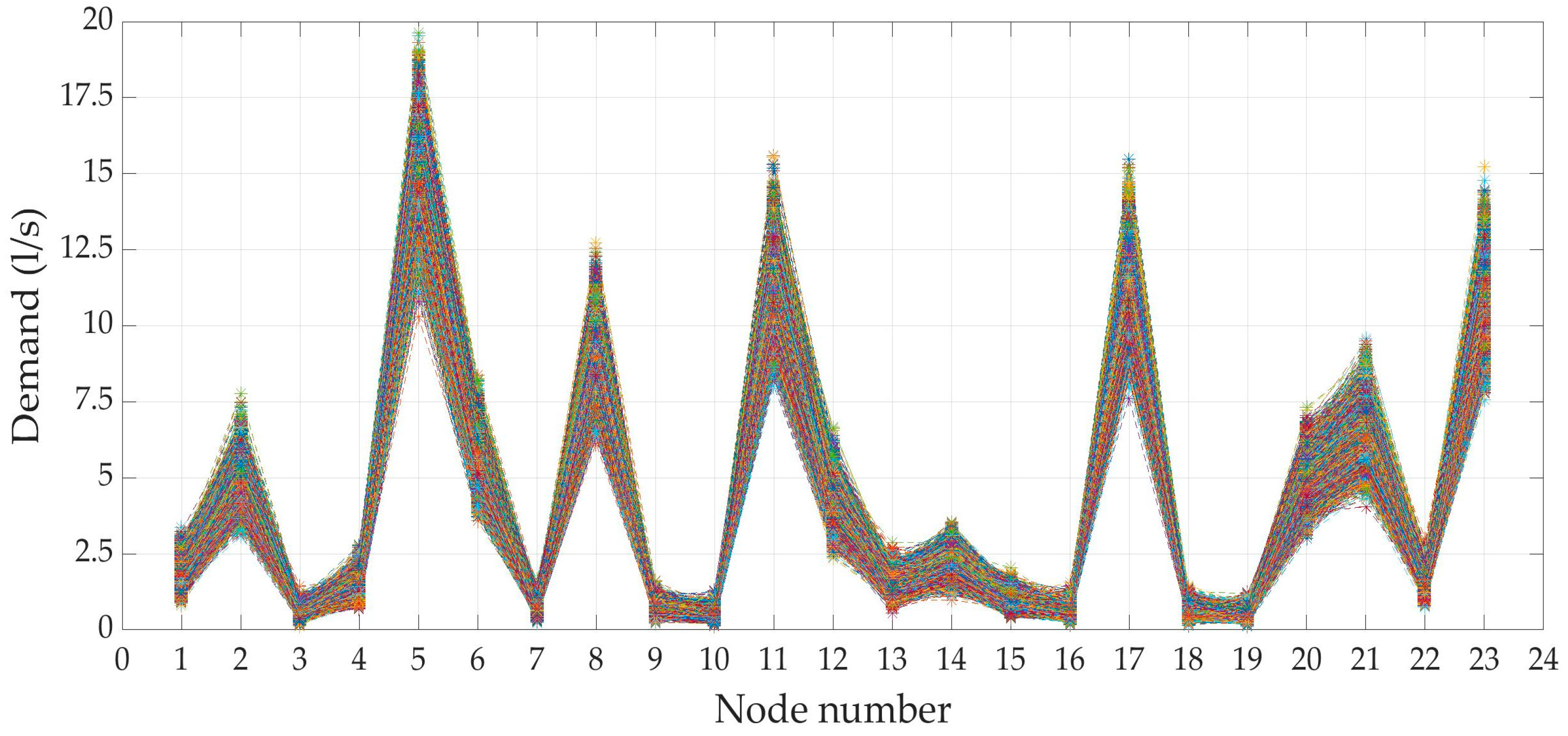
Also, in this case twelve-thousand scenarios were generated using the statistics estimated by the scaling laws, considering Gamma-distributed demands at each node, Figure 5. Differently from DemandA case, the value of generated data shows a great excursion between node and node due to the large variability in the number of users.

Similar to the previous case, Gamma distribution proves to be the best in fitting the generated data, as in Figure 6. Also, the INPUT distributions parameters, estimated by the scaling laws, well agree with the corresponding parameters of the generated scenarios distributions (OUTPUT), as in

Table 5. Gamma PDF parameters a and b input and output data at each node, DemandB.

	INPUT		OUTPUT			INPUT		OUTPUT
Node ID	a	b	a	b	Node ID	a	b	a	b
1	31.46	0.0575	31.46	0.0575	13	26.16	0.0544	26.16	0.0544
2	68.64	0.0726	68.65	0.0726	14	36.05	0.0599	36.05	0.0599
3	12.76	0.0439	12.76	0.0439	15	19.08	0.0495	19.09	0.0495
4	27.31	0.0551	27.31	0.0551	16	14.17	0.0453	14.17	0.0453
5	158.89	0.0933	158.90	0.0932	17	128.91	0.0876	128.92	0.0876
6	75.83	0.0748	75.84	0.0748	18	14.17	0.0453	14.17	0.0453
7	15.73	0.0467	15.73	0.0467	19	12.14	0.0433	12.14	0.0432
8	107.65	0.0830	107.66	0.0830	20	67.28	0.0721	67.28	0.0721
9	15.73	0.0467	15.73	0.0467	21	85.39	0.0775	85.40	0.0775
10	12.14	0.0433	12.14	0.0432	22	28.60	0.0559	28.61	0.0559
11	128.50	0.0875	128.51	0.0875	23	123.96	0.0866	123.97	0.0866
12	59.41	0.0695	59.42	0.0695	-	-	-	-	-

. In this case the correlation matrix of the generated scenarios almost matches perfectly with the input correlation matrix obtained from the scaling laws.

Table 6. Min, average, max values of input and output cross-correlation matrix, DemandB.

	E[ρ1] = 0.0043
	ρ Input Correlation Matrix (Scaling Laws)	ρ Output Correlation Matrix (Scenarios)
min	0.1627	0.1627
average	0.4329	0.4330
max	0.8261	0.8261

compares the minimum, average and maximum value of the input and output correlation matrices. The input and output correlation matrices are almost identical, but it should be noted that the correlation coefficient has very low values when considering node pairs with low number of users, intermediate values when one of the two has many users, higher values when the number of users is high for both. This responds to the fact that the correlation coefficient depends on the product of the number of users of the two considered nodes, see Equation (3).

3.3. Reduction of Demand Scenarios

The final phase of the procedure involves reducing the number of scenarios by aggregating them in relation to the distance of Kantorovich. For the application of the method the Euclidean norm was considered here. A reduced number of scenarios equal to 20 was chosen. In general, the choice of the number of scenarios should be based on the requirements of robust optimization problems and on the need for the reduced set to continue to describe the whole probability distribution of the demand at each node of WDN.

3.3.1. DemandA

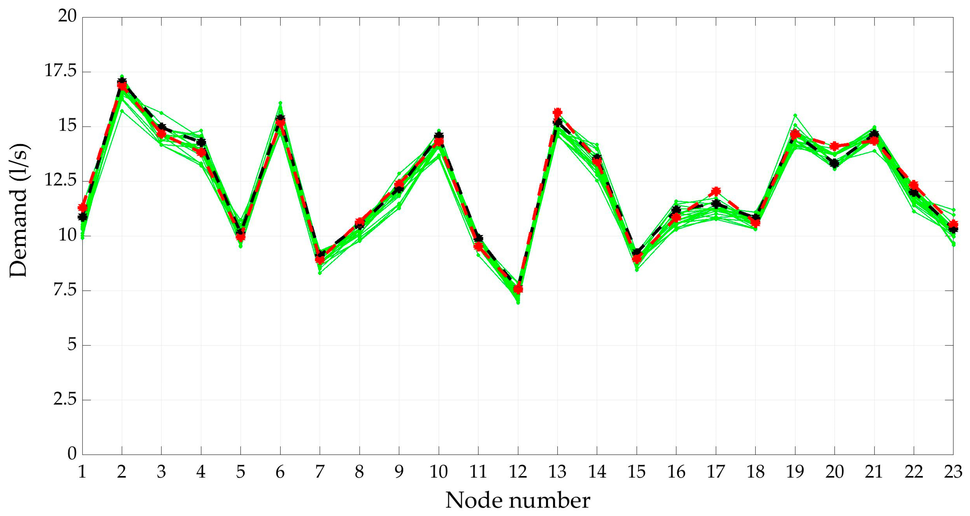
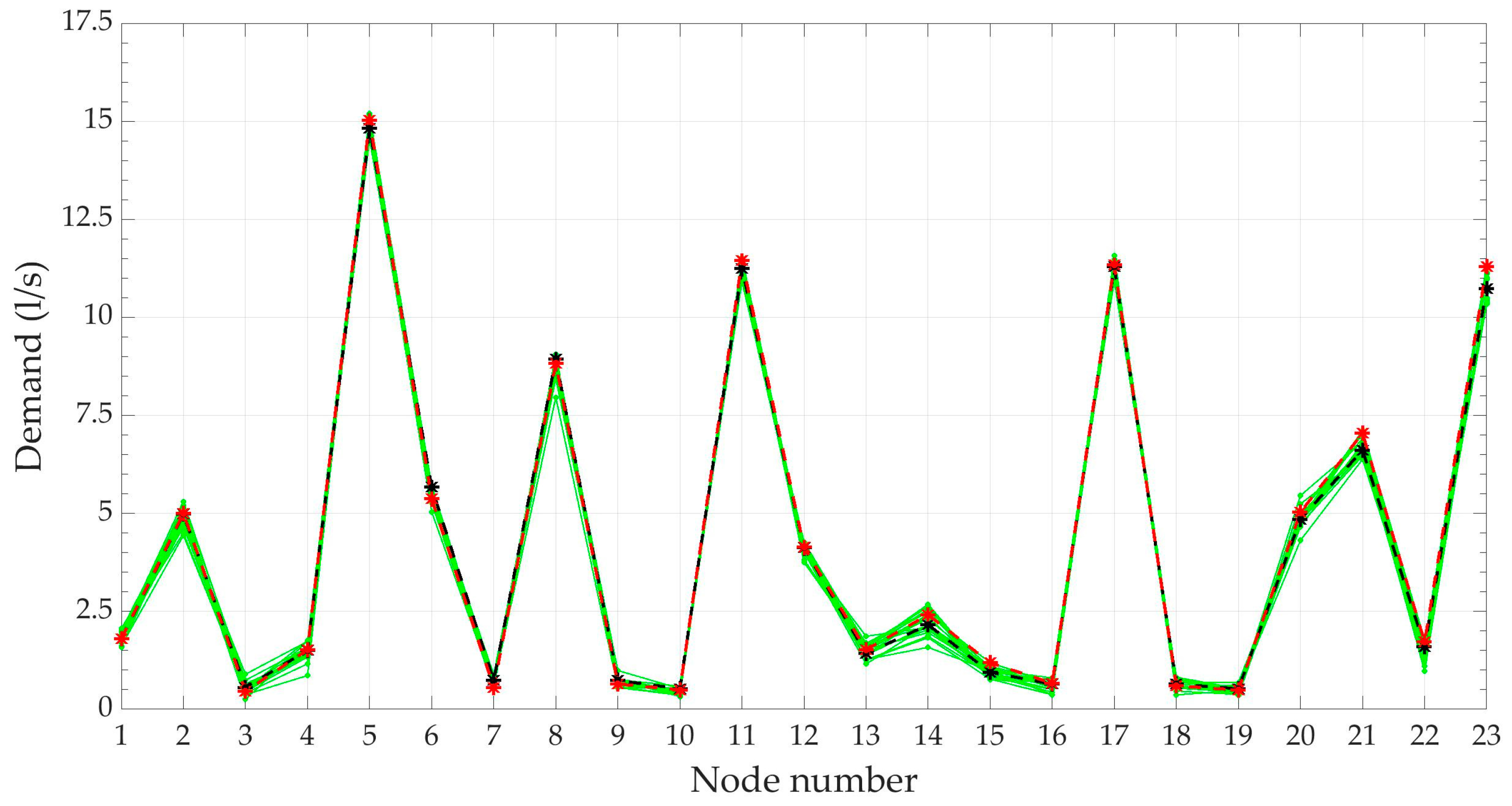
In Figure 7 the reduced demand scenarios are represented. The ‘mean scenario’, i.e., the one defined by the average nodal values of nodal demand is plotted by the black dotted line. The red dotted line indicates the most probable scenario, as reported in Figure 7. Mean and most probable scenarios, actually, do not coincide but are very close.

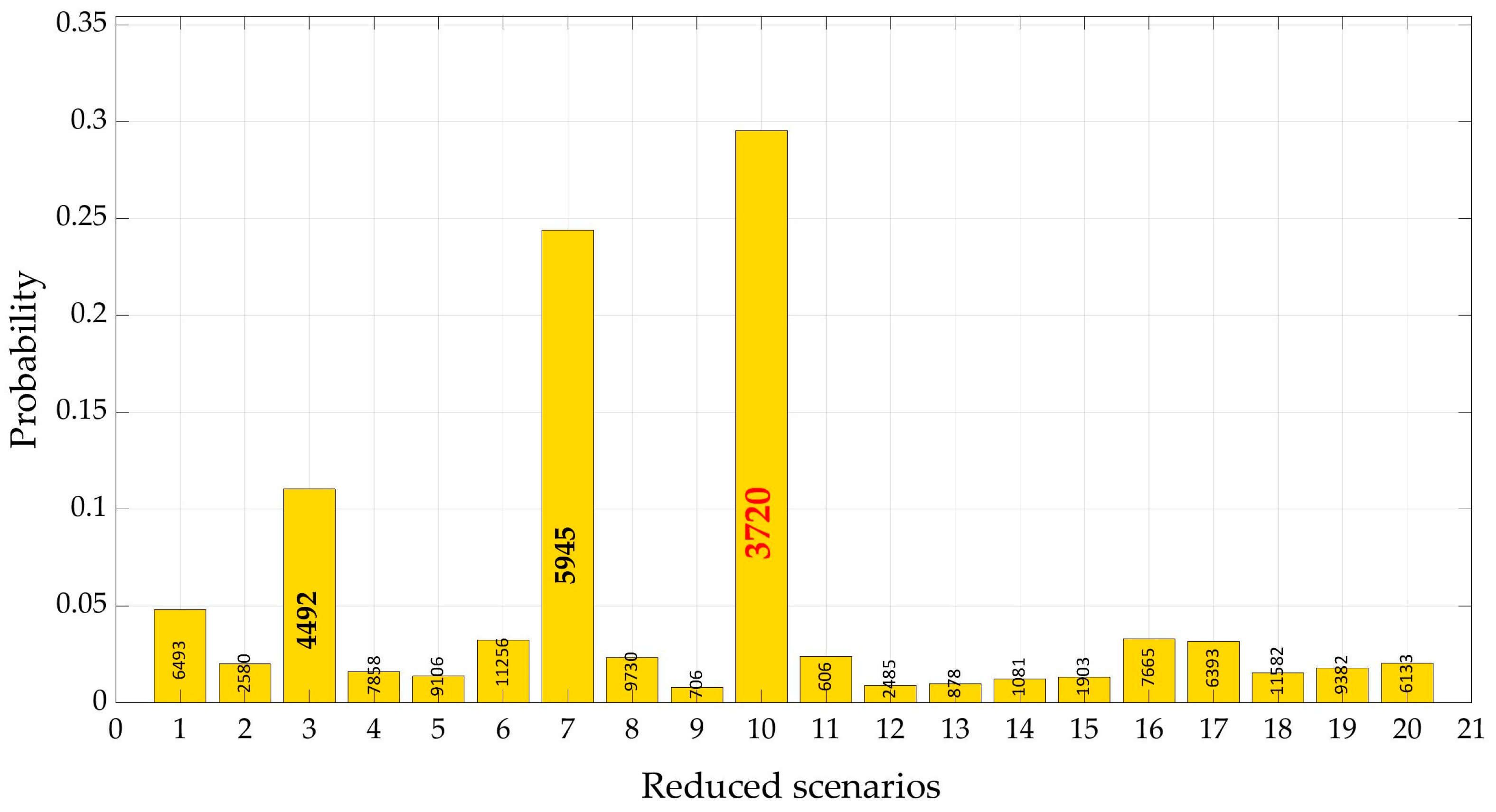
The most probable scenario in the set of generated ones, number 3720, shows a relevant weight, approximately equal to 0.3. Also, scenarios 5945 and 4492 exhibit significant weights, respectively 0.25 and 0.11. All the others have weights lower than 0.05, Figure 8. Nodal demands of the three most remarkable scenarios are reported in

Table 7. Nodal demand (l/s) of most probable scenarios and mean scenario, DemandA.

Node ID	Scenario 3720	Scenario 5945	Scenario 4492	Mean Scenario	Node ID	Scenario 3720	Scenario 5945	Scenario 4492	Mean Scenario
1	10.87	11.31	10.29	10.73	13	15.20	15.66	14.98	14.94
2	17.04	16.88	15.71	17.27	14	13.56	13.43	13.09	13.53
3	14.96	14.67	14.15	14.66	15	9.23	8.96	8.44	8.90
4	14.28	13.82	13.32	14.35	16	11.20	10.85	10.40	11.01
5	10.14	9.97	10.73	10.40	17	11.48	12.04	10.77	11.59
6	15.35	15.19	14.71	16.08	18	10.83	10.61	10.31	10.64
7	9.12	8.94	8.31	8.71	19	14.68	14.65	14.11	14.71
8	10.51	10.64	9.92	10.24	20	13.32	14.10	13.45	13.40
9	12.19	12.38	11.26	12.85	21	14.64	14.35	14.39	13.89
10	14.57	14.33	14.19	14.41	22	12.02	12.34	11.12	12.19
11	9.89	9.53	9.53	9.96	23	10.34	10.53	10.12	10.37
12	7.58	7.58	7.33	7.25	-	-	-	-	-

and compared with the average value of demand in each node, ‘mean scenario’. We can notice that all the selected scenarios are close to the mean one.

3.3.2. DemandB

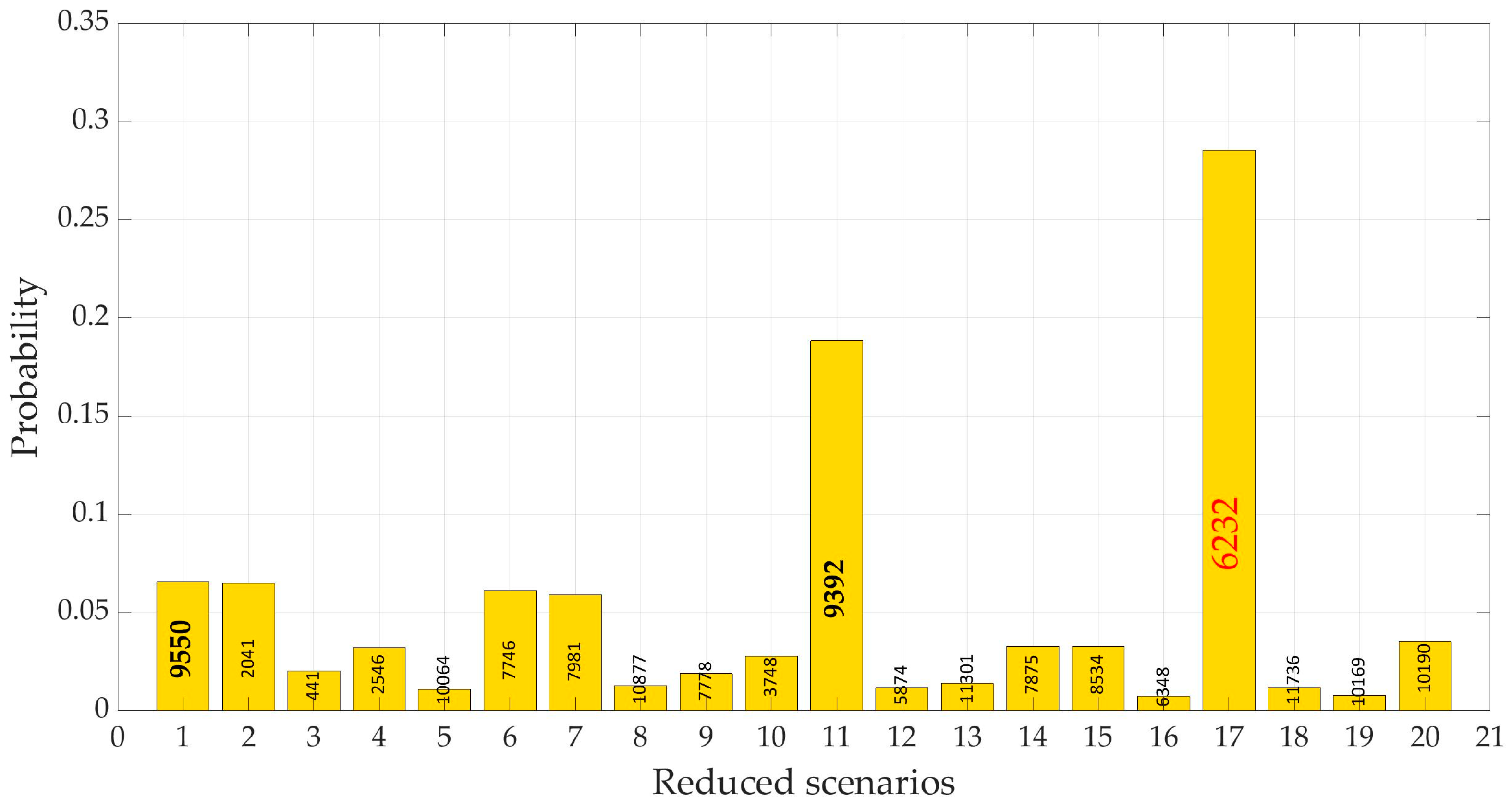
In Figure 9 the reduced demand scenarios are represented. In this case it is more difficult to distinguish one scenario from the other because of the big difference of average demand in the nodes Also, here there is no coincidence between the mean and the most probable scenario, number 6232 in the set of generated scenarios, but they are very close, as in Figure 10. In this case only another scenario, number 9392 has a weight greater than 0.1, but four scenarios exceed the probability threshold of 0.05. In

Table 8. Nodal demand (l/s) of most probable scenarios and mean scenario, DemandB.

Node ID	Scenario 6232	Scenario 9392	Scenario 9550	Mean Scenario	Node ID	Scenario 6232	Scenario 9392	Scenario 9550	Mean Scenario
1	1.81	1.81	1.75	1.80	13	1.42	1.52	1.27	1.39
2	4.98	5.01	4.80	4.71	14	2.16	2.41	1.58	2.13
3	0.56	0.46	0.64	0.48	15	0.94	1.19	0.99	1.06
4	1.50	1.52	1.39	1.55	16	0.64	0.66	0.65	0.58
5	14.82	15.03	14.55	14.92	17	11.29	11.34	11.24	11.16
6	5.67	5.38	5.38	5.62	18	0.64	0.60	0.83	0.64
7	0.73	0.56	0.59	0.68	19	0.52	0.49	0.45	0.55
8	8.94	8.82	8.45	8.82	20	4.85	5.04	4.86	4.91
9	0.73	0.65	0.76	0.69	21	6.61	7.05	6.65	6.59
10	0.52	0.50	0.34	0.46	22	1.60	1.72	1.53	1.10
11	11.25	11.45	11.04	11.24	23	10.73	11.30	11.12	10.64
12	4.13	4.14	4.04	4.05	-	-	-	-	-

nodal demands of the three most remarkable scenarios are reported and compared with the average value of demand in each node, the ‘mean scenario’.

3.4. Hydraulic Simulation with Scenarios from DemandA

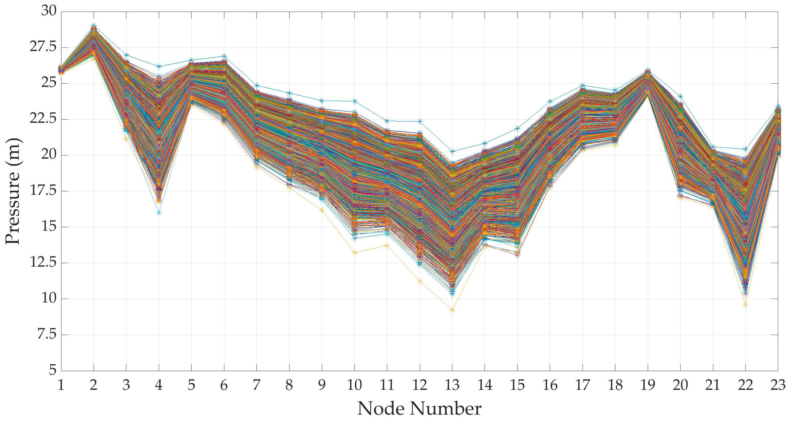
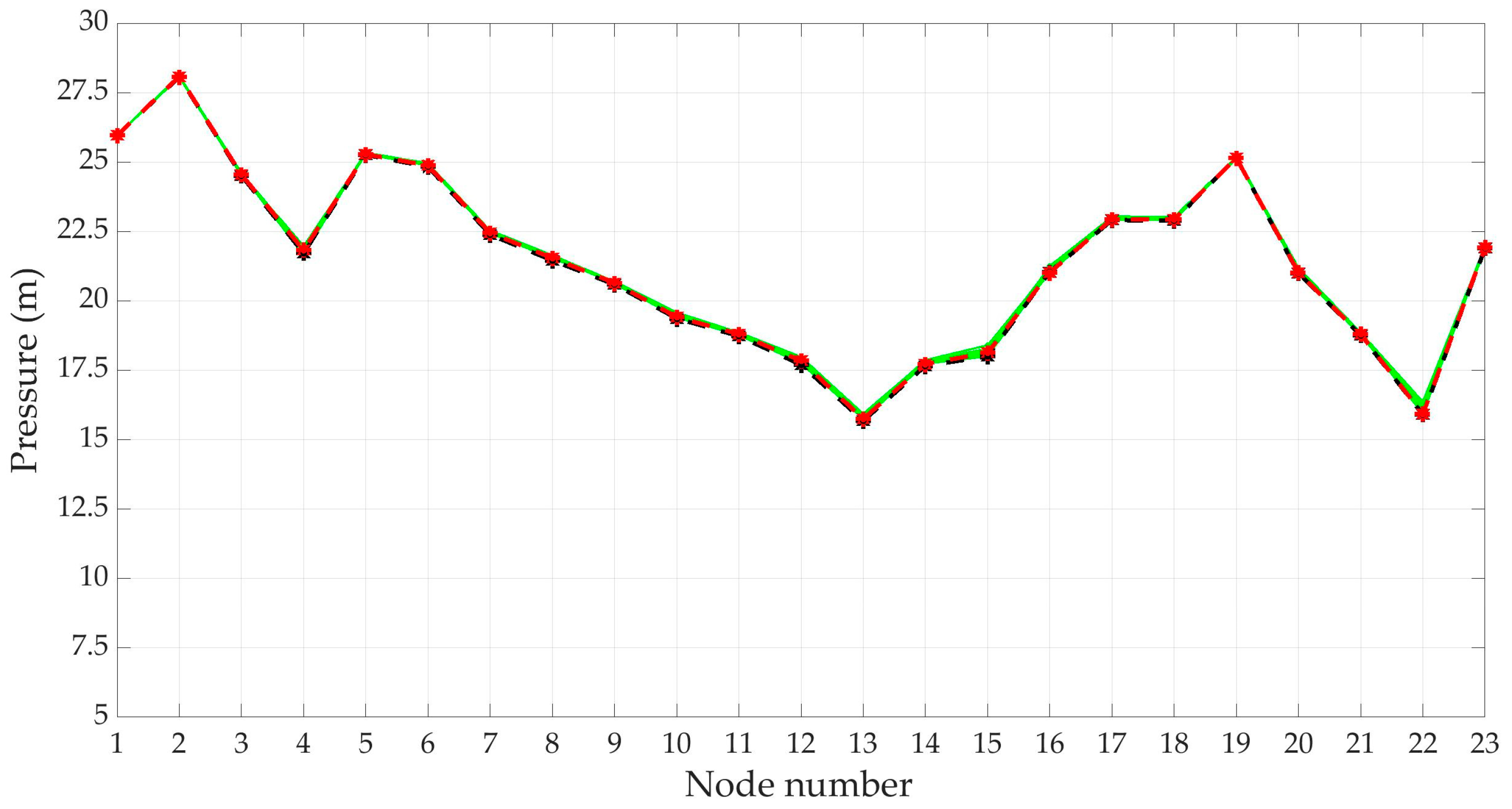
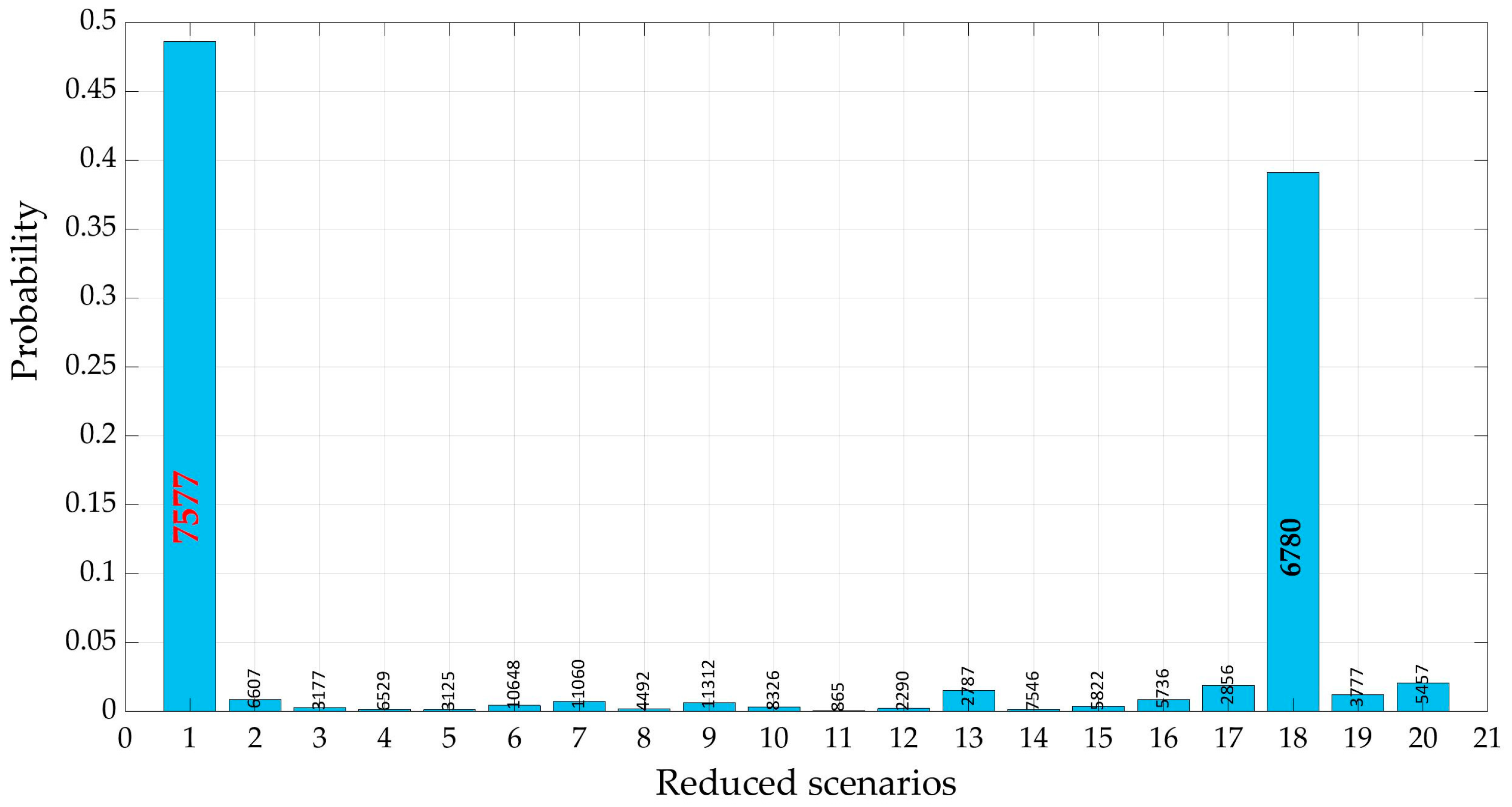
Water demand is the forcing parameter of a WDN and its natural variability is reflected on the variability of the quantities describing the hydraulic behavior of the whole system. The following question arises: how does the uncertainty of water demand determine the uncertainty of nodal pressure-heads and pipe flow-rate in a WDN? More specifically, how does the most probable water demand scenario coincide with the most probable pressure-head scenario? At this aim a set of pressure scenarios was derived from the set of generated demand scenarios in the DemandA case using a demand-driven hydraulic model based on the Global-Gradient algorithm proposed by Todini and Pilati [34]. Twelve-thousand pressure scenarios have been obtained for the Apulian network, as shown in Figure 11. This example does not take into account service constraints on each node. Actually, not all pressure scenarios deriving from demand scenarios can be significant in dealing with design and optimization problems. Using pressure-driven hydraulic models can allow the automatic filtering of unrealistic scenarios. The reduction algorithm was also carried on and twenty reduced scenarios with the corresponding probabilities were derived, as in Figure 12 and Figure 13.

The results show how the twelve-thousand scenarios generated, unlike the corresponding ones of the water demand, have the same ‘shape’, which depends on the geometrical and hydraulic characteristics of the WDN. From the results it is also possible to identify the nodes in which the pressure value shows greater variability: this can provide important support in positioning pressure gauges. Only two scenarios, number 7577, with weight approximately equal to 0.48, and number 6780, with weight about 0.39, remark a significant probability. All the others have probability lower than 0.025. In

Table 9. Nodal pressure (m) for different scenarios, DemandA.

Node ID	Scenario 7577	Scenario 6780	Scenario Mean Pressure	Scenario 3720	Scenario Mean Demand	Node ID	Scenario 7577	Scenario 6780	Scenario Mean Pressure	Scenario 3720	Scenario Mean Demand
1	25.965	25.962	25.963	25.966	25.965	13	15.754	15.904	15.684	15.839	15.723
2	28.077	28.052	28.061	28.085	28.070	14	17.727	17.850	17.661	17.697	17.692
3	24.548	24.543	24.512	24.592	24.534	15	18.135	18.278	18.001	18.107	18.041
4	21.829	21.852	21.714	21.963	21.755	16	21.023	21.222	21.042	21.138	21.068
5	25.280	25.314	25.254	25.289	25.267	17	22.946	23.040	22.908	22.930	22.927
6	24.875	24.929	24.829	24.888	24.849	18	22.933	22.966	22.895	22.906	22.911
7	22.453	22.522	22.383	22.449	22.407	19	25.149	25.185	25.147	25.139	25.155
8	21.545	21.618	21.454	21.522	21.483	20	21.019	21.193	20.997	21.021	21.026
9	20.647	20.691	20.592	20.694	20.620	21	18.794	18.859	18.768	18.731	18.785
10	19.421	19.553	19.366	19.501	19.404	22	15.926	16.363	15.908	16.111	15.959
11	18.808	18.864	18.731	18.855	18.764	23	21.919	21.976	21.894	21.862	21.909
12	17.846	17.902	17.700	17.901	17.747	-	-	-	-	-	-

pressure height in each node is reported for the two most probable pressure scenarios, for the scenario of mean pressure, for that of most probable demand (3720) and for the ‘mean scenario’. There are no significant differences between the highlighted scenarios.

4. Conclusions

This paper describes a complete procedure to generate and reduce the number of water consumption scenarios in order to represent the uncertainty due to the variability of demand in a WDN. Moreover, with this procedure, an objective measure of the probability of occurrence is related to each of the reduced scenarios.

For this purpose, the scaling laws, proposed by Magini et al. [1], prove all their potentials. In fact, they allow for a definition of the main statistical features of consumption for a different number of aggregated consumers, starting from the statistical characteristics of a typical user. Here, the features of a specific residential water demand are considered. However, if water demand is adequately typified, it is possible to examine different kinds of water use (commercial, public, …), different socio-economic categories and geographical locations.

One of the main goals of the proposed procedure is to correctly reproduce the statistical characteristics of water consumption in generating scenarios. The nodal water demand is supposed to follow a Gamma probability distribution with parameters dependent on the number of users. To respect cross-correlation between couples of water demand in the nodes, a generation algorithm based on the approach of Iman-Conover is implemented [8]. The generated water demand scenarios respect the hypothesized marginal probability distributions and reproduce the cross-correlations almost perfectly.

Regarding the scenario reduction, a probability/weight is defined for each of the reduced scenarios. Obviously, the probability/weight depends on the number of the reduced scenarios. The results show that the most likely scenario is close to the scenario represented by the average demand in each node. This fact may seem trivial, less trivial is the weight that is associated with them. We can observe that the reduced scenarios do not cover the whole set of generated scenarios, so they cannot completely describe the uncertainty of the demand, leaving out the tails of probability distributions, i.e., not considering the least likely scenarios. Probably, the relevant cross-correlation between couples of nodal water demand makes the Euclidean norm not perfectly suitable to describe the whole probability distributions, and the use of a different norm should be tested in future developments.

The reduction procedure has been applied also to the pressure-head scenarios which are derived from the generated demand. Also, in this case the most probable scenario is close to that defined by the average pressures in each node of the WDN, but it does not coincide with that produced by the most probable demand scenario.

The proposed procedure is certainly of considerable importance not only in the problems of robust optimization, but more in general in the modeling of the WDNs, both for their design and for their control.

References

- Magini, R.; Pallavicini, I.; Guercio, R. Spatial and Temporal Scaling Properties of Water Demand. J. Water Resour. Plan. Manag. 2008, 134, 276–284. [Google Scholar] [CrossRef]
- Bargiela, A.; Sterling, M. Adaptive forecasting of daily water demand. In Comparative Model for Electrical Load Forecasting; Bunn, D.W., Farmer, E.D., Eds.; John Wiley and Sons: New York, NY, USA, 1985. [Google Scholar]
- Perelman, L.; Housh, M.; Ostfeld, A. Robust optimization for water distribution systems least cost design. Water Resour. Res. 2013, 49, 6795–6809. [Google Scholar] [CrossRef] [Green Version]
- Xu, C.C.; Goulter, I.C. Reliability-based optimal design of water distribution networks. J. Water Resour. Plan. Manag. 1999, 125, 352–362. [Google Scholar] [CrossRef]
- Steffelbauer, D.; Neumayer, M.; Günther, M.; Fuchs-Hanusch, D. Sensor Placement and Leakage Localization considering Demand Uncertainties. Procedia Eng. 2014, 89, 1160–1167. [Google Scholar] [CrossRef]
- Pallavicini, I.; Magini, R.; Guercio, R. Assessing the spatial distribution of pressure head in municipal water networks. In Proceedings of the Eighth International Conference on Computing and Control for the Water Industry, Exeter, UK, 5–7 September 2005. [Google Scholar]
- Kapelan, Z.S.; Savic, D.A.; Walters, G.A. Multiobjective design of water distribution systems under uncertainty. Water Resour. Res. 2005, 41, W11407. [Google Scholar] [CrossRef]
- Iman, R.L.; Conover, W.J. A distribution-free approach to inducing rank correlation among input variables. Communun. Stat. 1982, 11, 311–334. [Google Scholar] [CrossRef]
- Tolson, B.A.; Maier, H.R.; Simpson, A.R.; Lence, B.J. Genetic algorithms for reliability-based optimisation of water distribution systems. J. Water Resour. Plan. Manag. 2004, 130, 63–72. [Google Scholar] [CrossRef]
- Vertommen, I.; Magini, R.; Cunha, M.D.C. Generating Water Demand Scenarios Using Scaling Laws. Procedia Eng. 2014, 70, 1697–1706. [Google Scholar] [CrossRef] [Green Version]
- Eck, B.; Fusco, F.; Taheri, N. Scenario Generation for Network Optimization with Uncertain Demands. In Proceedings of the 17th Water Distribution Systems Analysis Symposium, World Environmental and Water Resources Congress, Austin, TX, USA, 17–21 May 2015; pp. 844–852. [Google Scholar]
- Ridolfi, E.; Vertommen, I.; Magini, R. Joint probabilities of demands on a water distribution network: A non-parametric approach. AIP Conf. Proc. 2013, 1558, 1681–1684. [Google Scholar]
- Vertommen, I.; Magini, R.; Cunha, M.C.; Guercio, R. Water demand uncertainty: The scaling law approach. In Water Supply Systems Analysis: Selected Topics; Ostfeld, D.A., Ed.; InTech: London, UK, 2012; pp. 1–25. ISBN 978-953-51-0889-4. [Google Scholar]
- Vertommen, I.; Magini, R.; Cunha, M. Scaling Water Consumption Statistics. J. Water Resour. Plan. Manag. 2015, 141, 04014072. [Google Scholar] [CrossRef] [Green Version]
- Giustolisi, O.; Kapelan, Z.; Savic, D. Algorithm for Automatic Detection of Topological Changes in Water Distribution Networks. J. Hydraul. Eng. 2008, 134, 435–446. [Google Scholar] [CrossRef]
- Vershik, A. Kantorovich metric: Initial history and little-known applications. J. Math. Sci. 2006, 133, 1410–1417. [Google Scholar] [CrossRef]
- Blokker, E.J.M.; Vreeburg, J.H.G.; Dijk, J.C.V. Simulating Residential Water Demand with a Stochastic End-Use Model. J. Water Resour. Plan. Manag. 2010, 136, 19–26. [Google Scholar] [CrossRef]
- Creaco, E.; Alvisi, S.; Farmani, R.; Vamvakeridou-Lyroudia, L.; Franchini, M.; Kapelan, Z.; Savic, D. Preserving Duration-intensity Correlation on Synthetically Generated Water Demand Pulses. Procedia Eng. 2015, 119, 1463–1472. [Google Scholar] [CrossRef] [Green Version]
- Filion, Y.R.; Karney, B.W.; Moughton, L.; Buchberger, S.G.; Adams, B.J. Cross Correlation Analysis of Residential Demand in the City of Milford, Ohio. In Proceedings of the Water Distribution Systems Analysis Symposium, Cincinnati, OH, USA, 27–30 August 2006; ASCE: Reston, VA, USA, 2008. [Google Scholar]
- Filion, Y.; Adams, B.; Karney, B. Cross Correlation of Demands in Water Distribution Network Design. J. Water Resour. Plan. Manag. 2007, 133, 137–144. [Google Scholar] [CrossRef]
- Savic, D. Coping with risk and uncertainty in urban water infrastructure rehabilitation planning. In Proceedings of the Acqua e Città-1° Convegno Nazionale di Idraulica Urbana, Sorrento, Italy, 28–30 September 2005. [Google Scholar]
- Hutton, C.J.; Kapelan, Z.; Vamvakeridou-Lyroudia, L.; Savic, D. Dealing with Uncertainty in Water Distribution System Models: A Framework for Real-Time Modeling and Data Assimilation. J. Water Resour. Plan. Manag. 2014, 140, 169–183. [Google Scholar] [CrossRef]
- Kossieris, P.; Makropoulos, C. Exploring the Statistical and Distributional Properties of Residential Water Demand at Fine Time Scales. Water 2018, 10, 1481. [Google Scholar] [CrossRef]
- Ponomareva, K.; Roman, D.; Date, P. An algorithm for moment-matching scenario generation with application to financial portfolio optimization. Eur. J. Oper. Res. 2015, 240, 678–687. [Google Scholar] [CrossRef]
- Magini, R.; Capannolo, F.; Ridolfi, E.; Guercio, R. Demand uncertainty in modelling WDS: Scaling laws and scenario generation. WIT Trans. Ecol. Environ. 2016, 210, 735–746. [Google Scholar] [CrossRef]
- Mitra, S. Scenario Generation for Stochastic Programming; White Paper Series, Optirisk Systems, Domain: Finance Reference Number: OPT 004; SINTEF Technology and Society: Uxbridge, UK, 2006. [Google Scholar]
- Golub, G.H.; Van Loan, C.F. Matrix Computations, 3rd ed.; Johns Hopkins: Baltimore, MD, USA, 1996; ISBN 978-0-8018-5414-9. [Google Scholar]
- Ross, S.M. Introduction to Probability and Statistics for Engineers and Scientists, 5th ed.; Academic Press: Cambridge, MA, USA, 2014; ISBN 978-0-1239-48113. [Google Scholar]
- Ekstrom, P.A. A Simulation Toolbox for Sensitivity Analysis. Master‘s Thesis, Faculty of Science and Technology, Uppsala Universitet, Uppsala, Sweden, 2005. [Google Scholar]
- Dupacová, J.; Gröwe-kuska, N.; Römisch, W. Scenario reduction in stochastic programming. An approach using probability metrics. Math. Program 2003, 95, 493–511. [Google Scholar] [CrossRef]
- Morales, J.M.; Pineda, S.; Conejo, A.J.; Carrión, M. Scenario Reduction for Future Market Trading in Electricity Markets. IEEE Tras. Power Syst. 2009, 24, 878–888. [Google Scholar] [CrossRef]
- Heitsch, H.; Romisch, W. Scenario reduction in stochastic programming. Comput. Optim. Appl. 2003, 24, 187–206. [Google Scholar] [CrossRef]
- Giustolisi, O.; Laucelli, D.; Colombo, A.F. Deterministic versus stochastic design of water distribution networks. J. Water Resour. Plan. Manag. 2009, 135, 117–127. [Google Scholar] [CrossRef]
- Todini, E.; Pilati, S. A gradient algorithm for the analysis of pipe networks. In Computer Applications in Water Supply; Research Studies Press: Letchworth, UK, 1988. [Google Scholar]
Figure 1.
Flow-chart of the procedure for reducing scenarios.
Figure 2.
Apulian Network layout.
Figure 3.
Generated demand scenarios, DemandA.
Figure 4.
Gamma PDF distributions (cyan line) fitting demand data (grey bar), DemandA.
Figure 5.
Generated demand scenarios, DemandB.
Figure 6.
Gamma PDF distributions (cyan line) fitting demand data (grey bar) at each node, DemandB.
Figure 7.
Reduced demand scenarios, DemandA. Reduced nodal scenarios -> green line; average nodal values -> black dotted line; scenario with max probability -> red dotted line.
Figure 8.
Reduced demand scenarios’ probabilities, DemandA. Inside the bar is the number of the rank order of the generated scenario.
Figure 9.
Reduced demand scenarios, DemandB. Reduced nodal scenarios -> green line; average nodal values -> black dotted line; scenario with max probability -> red dotted line.
Figure 10.
Reduced demand scenarios’ probabilities, DemandB. Inside the bar is the number of the rank order of the generated scenario.
Figure 11.
Pressure headlines from the generated demand scenarios (DemandA).
Figure 12.
Reduced pressure headlines scenarios, DemandA. Total reduced scenarios -> green line; average nodal values -> black dotted line; scenario with max probability -> red dotted line.
Figure 13.
Reduced pressure scenarios’ probabilities DemandA. Inside the bar is the number of the rank order of the generated demand scenario.