Article

Synchronization Optimization of Pipeline Layout and Pipe Diameter Selection in a Self-Pressurized Drip Irrigation Network System Based on the Genetic Algorithm

1
Key Laboratory of Agricultural Soil and Water Engineering in Arid and Semiarid Areas, Ministry of Education, Northwest A&F University, Yangling 712100, China
2
State Key Laboratory Base of Eco-Hydraulic Engineering in Arid Area, Xi’an University of Technology, Xi’an 710048, China
*
Author to whom correspondence should be addressed.
Water 2019, 11(3), 489; https://doi.org/10.3390/w11030489
Submission received: 26 January 2019 / Revised: 27 February 2019 / Accepted: 3 March 2019 / Published: 8 March 2019
(This article belongs to the Section Water Use and Scarcity)

Abstract

:
A synchronous optimization method for self-pressure drip irrigation pipe network system is proposed. We have generalized the optimization design problem of the system and have established the mathematical models for the simultaneous optimization design of pipeline layout and pipe diameters. A genetic algorithm based on the infeasibility degree of the solution was used to solve the model. A typical example is used to validate the presented method. The method exhibits effective performance in the case studied. Designers can use the results of this study to efficiently design self-pressurized drip irrigation network systems.

1. Introduction

Most parts of Northwest China, especially Xinjiang, have year-round droughts and water shortages. In these regions, evaporation is considerably higher than the received rainfall [1,2,3]. Because of the extreme water shortage and high evaporation, agriculture there relies mainly on irrigation, and it is necessary to adopt efficient irrigation techniques to use limited water to meet crop water requirement while reducing evaporation.
Among numerous irrigation techniques, drip irrigation is considered to be an efficient and water-saving irrigation technique. Drip irrigation system allows water to drip slowly and accurately to the root zone of crops through emitters [4], significantly reducing the amount of irrigation water as well as decreasing the amount of water that leaches beneath the root zone [5]. Therefore, water utilization efficiency can be greatly improved.
In order to further improve the water use efficiency and achieve the purpose of increasing crop production, plastic film mulching technology and drip irrigation are combined (mulched drip irrigation (MDI)) to give full play to their respective advantages in arid and semiarid regions [6,7]. Plastic film mulching can conserve soil moisture and increase the productivity of crops [8]. Mulch also shields the soil surface against solar radiation, thereby buffering soil temperature fluctuations [6]. In addition, plastic film mulching assists weed control [9,10].
The MDI has been widely applied in Xinjiang, China in recent years [11,12], and the construction of large-scale (larger than 60 hectares) drip irrigation pipe network systems has progressed rapidly [13,14]. However, the design of drip irrigation pipe network systems still relies on time-consuming and laborious empirical methods, which can obtain optimal design schemes only with difficulty. Therefore, efficient methods for drip irrigation pipe network design are urgently required.
With the development of computer technology, numerous scholars have discussed the application of computer technology in the optimization of pipe network systems. Scholars have made considerable progress with numerous computer-based methods, such as linear programming (LP), nonlinear programming (NLP), and dynamic programming (DP). Giménez et al. [15] proposed a two-level DP method to deal with the optimal design of sewerage networks. The LP gradient method was presented for the optimal design of a water distribution system, and a satisfactory hydraulic design was obtained [16]. Theocharis et al. [17] proposed the Theocharis’ simplified NLP (TSNLP) method for irrigation pipe network design. They compared the results of their method with the results obtained from the LP and Labye methods and proved the simplicity and effectiveness of TSNLP. Arai et al. [18] applied a fuzzy LP method to achieve multiple-objective optimization of water operations in a water supply and distribution system. The fuzzy LP was used for achieving a balance among multiple objectives. The aforementioned methods have been used to address pipe network optimization problems. However, these methods are typically very complex, and their numerical solutions involve copious calculations, especially in the case of large and complicated pipe networks [17].
In the past 20 years, numerous heuristic algorithms, such as the simulated annealing [19], tabu search [20,21,22], genetic [23], particle swarm optimization (PSO) [24], ant colony [25], harmony search [26], and shuffled frog-leaping [27] algorithms, have been proposed and proved to be efficient and reliable for solving complex optimization problems [28,29,30,31,32,33]. Therefore, pipe network systems should be designed with advanced optimization algorithms.
Several studies have optimized pipe networks by using heuristic algorithms. Simpson et al. [34] applied a genetic algorithm (GA) with the standard three operators to obtain optimal designs for water distribution networks. They proved the effectiveness and high efficiency of the GA in finding global optimal or near-optimal solutions. Savic and Walters [35] developed a GA program called GANET to design low-cost water distribution networks and indicated that the GA was particularly suited to this type of problem. Cunha and Sousa [36] then also considered the least cost of a pipe network as the design objective. They applied a simulated annealing algorithm to obtain the least-cost design of a looped water distribution network, proving that this heuristic method can provide high-quality solutions for network design problems. Geem et al. [26] introduced a new heuristic optimization algorithm called harmony search for the pipe network design problem. The harmony search algorithm generated numerous near-optimal solutions and quick convergence. Chung and Lansey [37] developed an improved shuffled frog-leaping algorithm for solving a general large-scale water supply system model with the objective of minimizing the total system cost. Trigueros [38] used a modified PSO method for optimizing reused water networks and obtained reliable global results. However, almost all of the aforementioned studies optimized ideal problems and did not aim the practical complex problems. They are mainly focused on multinode water supplying problems [28,33,34,35,36,37] and water/wastewater allocation planning problems [38]. Only a few studies have been conducted on the optimization design of drip irrigation pipe networks. More such studies are urgently required.
Taking the optimization design of drip irrigation pipe network system in Xinjiang as a practical example, this study focuses on the following contents: (a) considerations and problems of the optimization of an actual self-pressurized drip irrigation pipe network system; (b) establishment of the mathematical models of the system; (c) a solution method for the model.

2. Materials and Methods

2.1. Problem Description and Generalization

A large-scale drip irrigation pipe network system typically consists of main pipes, sub-main pipes, branch pipes, lateral pipes, control head (e.g., filters, air release valves, metering valves, non-return valves), and some other equipment. A comb-shaped pipe network layout is most commonly used in the design of drip irrigation pipe network systems in Xinjiang. To simplify the problem studied, the field has a regular shape. The comb-shaped drip irrigation pipe network system is illustrated in Figure 1. Considering economic factors, the branch pipes lie on both sides of the sub-main pipe, and the lateral pipes lie on both sides of the branch pipe in areas with relatively flat terrain.
The objective of pipe network optimization is generally directly or indirectly related to the total cost of the pipe network. The total cost of the pipe network is a function of pipe materials, lengths, and diameters. For a given type of pipe, the total cost of the pipe network is proportional to the lengths and diameters of the pipes. For a drip irrigation network system, a close connection exists between the pipe length and pipe diameter at all levels. In our study, we assumed that the sub-main pipes and branch pipes are equally spaced. As displayed in Figure 1, the spacing of the branch pipes affects the length of the lateral pipes. When the spacing of the branch pipes increases, the lengths of the corresponding lateral pipes and the number of emitters controlled by the lateral pipes increase. The aforementioned changes lead to an increase in the discharges of the lateral pipes. Therefore, the diameters of the lateral pipes must be enlarged. Moreover, an increase in the spacing of the sub-main pipes requires an increase in the lengths of the branch pipes. The number of lateral pipes controlled by the branch pipes also increase. Therefore, the discharges of the branch pipes increase, which finally causes the enlargement of the diameters of the branch pipes. Therefore, how to reasonably determine the layout and diameter of the sub-main and branch pipes for minimizing the investment is an urgent problem that must be solved.
When determining a solution to the aforementioned problem, the working scheme of the pipelines at all levels must be considered. In the proposed drip irrigation pipe network system, continuous irrigation was adopted for the main pipe and rotational irrigation was adopted for the sub-main and branch pipes. Because only the entrance of each branch pipe is equipped with valves, all the lateral pipes controlled by branch pipework in a continuous irrigation scheme. Furthermore, considering the economic reasons in the design, each sub-main pipe generally supplies water to a maximum of two branch pipes simultaneously. The grouping method of rotation irrigation of the two branch pipes that work simultaneously is shown in Figure 2. The number of sub-main pipes working simultaneously is determined by the design irrigation period, duration of irrigation, and the number of branch pipes that work simultaneously on the sub-main pipe. Considering the most unfavorable conditions, the neighboring sub-main pipes are assumed to work simultaneously.

2.2. Mathematical Models

The design of a drip irrigation network system is a very complicated problem. For the convenience of analyzing our problem and describing our optimization process, we divided the whole pipe network (WPN) system into the branch–lateral pipe network (BLPN) and main–sub-main pipe network (MSMPN) subsystems according to the characteristics of rotational or continuous irrigation of pipelines at all levels. We formalized the mathematical optimization models for the BLPN and MSMPN subsystems. Finally, the mathematical optimization model for the WPN system was constructed by integrating the two subsystems for the overall synchronized optimization of the pipeline layout and pipe diameter.

2.2.1. Mathematical Model for the BLPN Subsystem

The optimization design of the BLPN system mainly involves determining the lengths and section diameters of the branch and the lateral pipes. For simplicity, the section between the two adjacent emitters connected to the lateral pipe is regarded as a lateral pipe section. Moreover, the section between the two adjacent lateral pipes connected to the branch pipe is regarded as a branch pipe section.
Considering the practical application, the diameters of the lateral pipe remained constant, and all the lateral pipes in the BLPN subsystem were selected from commercially available drip belts with the same pipe specification. The branch pipes are considered to consist of several sections with variable diameters. Only one commercially available pipe diameter was adopted for each branch pipe section. Therefore, the diameter optimization of the BLPN subsystem only determines the diameter of each section of the branch pipes.

Objective Function

The objective function of optimizing the BLPN subsystem is to minimize the cost of a branch pipe and the lateral pipes connected to it.
min F b l = i = 1 N b L b i C b i + ( N l l L l l + N l r L l r ) C l
where Fbl is the total cost (Yuan) of the pipes in a BLPN subsystem; Nb is the number of branch pipe sections; L b i and C b i are the length (m) and unit price (Yuan/m) of the branch pipe section i, respectively; Nll and Nlr are the total number of lateral pipes on the left and right side of the corresponding branch pipe, respectively; Lll and Llr are the lengths (m) of the lateral pipes on the left and right sides of the corresponding branch pipe, respectively; Cl is the unit price (Yuan/m) of the lateral pipe.

Constraints

Constraints of the allowable head difference in the BLPN subsystem: Considering that no pressure-regulating valve exists at the entrance of the lateral pipe, the maximum head difference of the emitters in the BLPN subsystem must be controlled within the allowable head difference to ensure irrigation uniformity. This study considered the difference between the maximum and minimum heads of all the emitters in the BLPN subsystem as constraints.
Δ H = H max H min [ Δ H ]
where ∆H is the difference between the maximum and minimum heads (m) of all the emitters in the BLPN subsystem; Hmax and Hmin are the maximum and minimum work head (m) in all the emitters, respectively; [∆H] is the allowable head difference (m) of the BLPN subsystem.
For conveniently calculating ∆H, the concept of relative pressure head of the emitter can be introduced. When the pressure head at the inlet of the branch pipe is zero, the corresponding pressure head of each emitter is defined as the relative pressure head. The relative pressure head of the emitter k is expressed as follows:
H k = H 0 j = 1 N b k ( α b f b l b j Q b j m D b j b + i b l b j ) j = 1 N l k ( α l f l l l j Q l j m D l j b + i l l l j )
where Hk is the relative pressure head (m) of the emitter k, H0 is the pressure head (m) at the entrance of the branch pipe, Nbk is the number of branch pipe sections passed from the inlet of the branch pipe to the emitter k, Nlk is the number of lateral pipe sections passed from the inlet of the lateral pipe to the emitter k, and αb and αl are the expansion factors of the frictional head loss after considering the local head loss. In this study, αb = 1.1; αl = 1.1; fb and fl are the friction coefficients of the frictional head loss; Qbj and Qlj are the discharges (m3/s) of section i of the branch and lateral pipes, respectively; Db and Dlj are the diameters (mm) of section i of the branch and lateral pipes, respectively; m is the discharge index; b is the diameter index; ib and il are the slopes along the branch and lateral directions, respectively; lbj and lbj are the lengths (m) of section i of the branch and lateral pipes, respectively.
Constraints of the distribution pressure: For a self-pressurized drip irrigation network, the pressure of the headwork is basically constant. A reasonable pressure distribution ratio should be set up for the BLPN subsystem to ensure that it can satisfy the emitters’ working requirements and is as economical as possible. The maximum pressure at the inlet of the branch pipes should not be higher than the pressure distributed.
H b _ max H b _ d i s
where Hb_max is the maximum pressure at the branch inlet (m) and Hb_dis is the pressure (m) distributed to the BLPN subsystem. Hb_dis is calculated as follows:
H b _ d i s = R d i s H h e a d
where Rdis is the ratio of the pressure of the BLPN subsystem (Hb_dis) to the pressure of the headwork (Hhead).
Constraints of the maximum allowable current velocity for the branch pipes: To prevent a high current velocity from causing excessive wear and damage to the pipeline, the actual current velocity in each pipe section must not exceed the maximum allowable value (2.0 m/s velocity safety limit). The velocity constraint is expressed as follows:
V i V max i = 1 , 2 , , ( N b + N l )
where Vi is the actual current velocity (m/s) in pipe section i; Vmax is the maximum allowable current velocity (m/s); Nb and Nl are the total lateral and branch pipe sections, respectively.
Diameter constraints: Along the direction of the current, the diameter of the previous section in each branch pipe must be no less than that of the following section. The diameter constraint is expressed as follows:
D i D i + 1 i = 1 , 2 , , N b
where Di is the diameter (mm) of the branch pipe section i, and Di+1 is the diameter (mm) of the branch pipe section i + 1.

2.2.2. Mathematical Model for the MSMPN Subsystem

The optimization design of the MSMPN subsystem mainly involves determining the lengths and diameters of all the sections of the main and sub-main pipes. Similar to the BLPN subsystem, the pipe section between the two adjacent branch pipes connected to the sub-main pipe is regarded as a sub-main pipe section. Moreover, the pipe section between the two adjacent sub-main pipes connected to the main pipe is regarded as the main pipe section. Both the main and sub-main pipes are considered to consist of several sections with variable diameters, and only one commercially available pipe diameter is adopted for each pipe section.

Objective Function

The minimum cost of pipes in the MSMPN subsystem is the objective function, which is defined as follows:
min F m s = i = 1 N m C m i l m i + k = 1 N s n j = 1 N s C s k j L s k j
where Fms is the total cost (Yuan) of the main and sub-main pipes in the MSMPN subsystem; Nm is the total number of main pipe sections; Cmi and lmi are the unit price (Yuan/m) and length (m) of the main pipe section i, respectively; Nsn is the total number of sub-main pipes; Ns is the total number of sections of each sub-main pipe; Cskj and lskj are the unit price (Yuan/m) and length (m) of section j on the sub-main pipe k, respectively.

Constraints

Constraints for the working pressure head: The pressure head at the inlet of each branch pipe must satisfy the following requirement:
h max E 0 j = 1 N mk ( α m f m l m j Q m j m D m j b + i m l m j ) j = 1 N s k ( α s f s l s j Q s j m D s j b + i s l s j ) h min
where hmax is the maximum allowable pressure head (m) at the inlet of each branch pipe; hmin is the minimum required pressure head (m) at the inlet of each branch pipe; E0 is the pressure head (m) at the inlet of the main pipe; Nmk is the total number of main pipe sections passed from the inlet of the main pipe to the inlet of the branch pipe k; Nsk is the total number of sub-main pipe sections passed from the inlet of the main pipe to the inlet of the branch pipe k; im and is are the slopes along the direction of the main and sub-main pipes, respectively, where positive values are taken along the slope, and negative values are taken against the slope; lmj and lsj are the lengths (m) of section j of the main and sub-main pipes, respectively; αm and αs are the expansion factors of the frictional head loss after considering local head loss. In this study, αm = 1.1; αs = 1.1; fm and fs are the friction coefficients of the frictional head loss; Qmj and Qsj are the discharges (m3/s) of section i of the main and sub-main pipes, respectively; Dmj and Dsj are the diameters (mm) of section i of the main and sub-main pipes, respectively; m is the discharge index; b is the diameter index.
Constraints for the hydrostatic pressure head: The maximum hydrostatic pressure head in the MSMPN subsystem must not exceed the pressure capacity of the pipe adopted.
h sta = j = 1 N m ( α m f m l m j Q m j m D m j b + i m l m j ) + j = 1 N s ( α s f s l s j Q s j m D s j b + i s l s j ) H c
where hsta is the maximum hydrostatic pressure head (m) in the MSMPN subsystem, and Hc is the pressure capacity (m) of the pipe adopted. Other symbols have the same meanings as previously discussed.
Constraints for the pressure balance at the entrance of each branch pipe: When two branch pipes attached on one sub-main pipe are working simultaneously, the pressure difference at the entrance of the two branch pipes must be less than a certain value. This measure ensures the uniformity of irrigation and reduces the adverse effects caused by pressure imbalance in the sub-main pipe. According to engineering experience, the pressure difference must not exceed 20% of the minimum pressure of all entrances of the branch pipes. The constraint for the pressure balance is defined as follows:
h d i f H b _ min
where hdif is the maximum pressure difference (m) at the entrance of the two branch pipes working in a sub-main pipe, and Hb_min is the minimum pressure (m) at the inlet of all the branch pipes.
Constraints for the maximum allowable current velocity and diameters: The constraints for the maximum allowable current velocity and diameters of pipes are similar to the related constraints of branch pipes (Equations (6) and (7)).

2.2.3. Mathematical Model for the WPN System

The WPN system consists of one MSMPN subsystem and many BLPN subsystems. The mathematical models for the MSMPN and BLPN subsystems have already been discussed previously. In the optimization of the WPN system, Nm, Ns, and Rdis are used as links to achieve a suitable combination of the MSMPN and BLPN subsystems. The values Nm and Ns can determine the layouts of the MSMPN and BLPN subsystems. The value of Rdis determines the distributed pressure head of both the subsystems, thereby affecting the selection of the pipe diameter. If Nm and Ns are known, the lengths of the main pipe and sub-main pipe sections can be calculated for a given designed field. Then, we can determine the lengths of the branch pipes and lateral pipes because the lengths of the branch and lateral pipes are approximately equal to the lengths of main and sub-main pipe sections, respectively. Thus, the layouts of MSMPN and BLPN subsystems can be determined.

Objective Function

Consider the minimum investment in the WPN system as the objective function, which is defined as follows:
min F W P N = F m s + 2 N m N s F b l
where FWPN is the total cost (Yuan) of all the pipes in the WPN system; Fms is the total cost (Yuan) of the main and the sub-main pipes in the MSMPN subsystem; Nm is the total number of main pipe sections; Ns is the total number of sub-main pipe sections; Fbl is the total cost (Yuan) of the branch and lateral pipes in a typical BLPN subsystem.

Constraint Conditions

Total head restriction: The sum of the working pressure of the emitter; the friction head losses of the lateral, branch, sub-main, and main pipes; the local head loss of relevant locations, and the elevation differences must not exceed the pressure provided by the headwork.
H e m i + H l o s s + E d i f < H h e a d
where Hemi is the working pressure of the emitter (m); Hloss is the sum of the friction loss and local head loss of all the pipes (m); Edif is the terrain height difference (m); Hhead is the head pressure at the headwork (m).

2.3. Method of the Model Solving

2.3.1. GA Based on the Infeasibility Degree (IFD) of the Solution

A GA [23] is a heuristic search algorithm that simulates biological evolution in nature. A population evolves because its fittest members reproduce. The fitness function is used to simulate the survival of the fittest. Thus, after numerous iterations, optimal solutions are obtained [39,40]. Numerous papers on GAs have been published. GAs have received considerable attention and are widely used in various research fields. Moreover, GAs superior exhibit superior results [41,42,43,44,45,46,47]. Compared with most other heuristic algorithms, the GA has a stable performance and superior global search ability [48,49]. In this study, the GA served as the optimization algorithm.
Numerous constraints must be managed when solving models. The general method of dealing with constraints is by penalizing infeasible solutions, that is, penalty function methods [50]. However, setting an appropriate penalty factor for obtaining a feasible global optimum solution is challenging. Specifically, the performance of penalty function methods is not always satisfactory in handling highly constrained or nonconvex constrained optimization. Moreover, penalty function methods distort the characteristics of the objective function to a certain extent [51]. Therefore, in this study, the constraints are addressed using the IFD method [52] instead of penalty function methods. The IFD method is simple and effective. It screens and improves populations by comparing the IFD of solution ϕ with the threshold ϕcrit. The term ϕ is defined as follows:
ϕ ( x i ) = j = 1 J [ min { 0 , g j ( x i ) } ] 2 + k = 1 K [ h k ( x i ) ] 2
where J and K are the total number of inequality and equality constraints, respectively, and g j and h k are the inequality and equality constraints of the problem, respectively.
The threshold ϕcrit is given by Equation (15).
ϕ c r i t = 1 T ( i = 1 N I N D ϕ ( x i ) ) / N I N D
where T is a coefficient that increases from Tstart to Tend with the GA’s iteration to control the acceptable bound of the infeasible solutions, and NIND is the number of individuals in the population.
By comparing ϕ with ϕcrit, one can determine whether an infeasible solution is accepted (when ϕϕcrit) or rejected (when ϕϕcrit). The rejected infeasible solutions are replaced by the most feasible solutions in the current population, whose size remains fixed.
The basic flowchart of the GA based on the IFD method is displayed in Figure 3.

2.3.2. Overall Solution Process of the Model

This study used a GA based on the IFD method to solve the pipe network optimization model.
First, according to the known Lf, Wf, lb_min, lb_max, ll_min, ll_max (the meanings of these abbreviations are comprehensively listed in “Abbreviations”) values, the values of Nm_min, Nm_max, Ns_min, and Ns_max can be obtained. One can also determine a reasonable range of Rdis from engineering experience. In this study, Rdis had values ranging from 0.25 to 0.45 in increments of 0.01. Nm, Ns, and Rdis were set as variables, and all combinations of Nm, Ns, and Rdis were generated using a complete enumeration method. The proposed GA was used to optimize the BLPN subsystem under each combination, and the optimal results of the BLPN system were saved. These results were used in the WPN system optimization procedure to avoid the repeated computation of equivalent individuals due to the same combinations of Nm, Ns, and Rdis in the GA’s populations. The solution process is illustrated in Figure 4.
The detailed design process for the code, fitness, and IFD of the GA in the BLPN and MSMPN subsystems and WPN system is described in the following text.

GA for Optimizing the BLPN Subsystem

Code design for optimizing the BLPN subsystem: To facilitate the installation of pipelines and reduce the local head loss, each branch pipe is assumed to consist of a maximum of four sections with different diameters (Figure 5). The set of commercially available diameters (in millimeters) for branch pipes is S = {32, 40, 63, 75, 90, 110, 125}, as listed in Table 1. For reducing the infeasible solution and meeting the pipe diameter constraints, the ratio factors (α1, α2, and α3), which reflect the length of each section, are used as decision variables for coding. The coding string of the branch pipes is displayed in Figure 6. The coding string is called a chromosome in the GA. The chromosome consists of four genes. The first gene is the code for the position number of the diameter of the end section of the branch pipe in the pipe diameter set S. The second, third, and fourth genes are the codes for α1, α2, and α3, respectively. Each coded value is an integer between 0 and 100.
Fitness function for optimizing the BLPN subsystem: The objective function Fbl is set as the fitness function (Equation (1)). The smaller the value of Fbl, the better is the solution.
IFD for the optimization of the BLPN subsystem: The IFD of the solution of the BLPN subsystem is used to address the constraint problems in it. The maximum head difference in the BLPN subsystem must not exceed the allowable head difference (Equation (2)), and the pressure at the entrance of each branch pipe must not be higher than the distributed water head (Equation (4)). These two constraints are inequality constraints, which are expressed as follows:
g 1 ( x i ) = H a d H d i f
g 2 ( x i ) = H dis H b _ e n t H e m i
where Had is the allowable head difference (m) in the BLPN subsystem, Hdif is the maximum head difference (m) in the BLPN subsystem, Hdis is the head (m) distributed to the BLPN subsystem, Hb_ent is the head (m) at the entrance of the branch pipe, and Hemi is the working pressure head (m) of the emitter.

GA for Optimizing the MSMPN Subsystem

Code design for optimizing the MSMPN subsystem: For ensuring the comprehensiveness and effectiveness of the search space, the diameters of all the sections of sub-main and main pipes are considered for code design. The chromosome consists of Nm(Ns + 1) genes (Figure 7).
The length of the code string varies to reflect the variance in Nm and Ns. The entire code string is binary coded. The first Nm genes represent whether the diameter of each main pipe section varies or not compared with that of the section behind it along the direction of the flow in the pipes. The number “0” represents “remain unchanged,” whereas the number “1” represents “change”-the diameter number of current section equals the diameter number of the following section plus 1. The end section of the main pipe changes according to the diameter at the entrance of the corresponding sub-main pipe. The following Ns × Nm genes represent whether the position number of the diameter of the current sub-main pipe section varies or not compared with that of the section behind it. The numbers “0” and “1” have the same meaning as previously explained. The end section of the sub-main pipe changes according to the diameter at the entrance of the corresponding branch pipe.
Fitness function for optimizing the MSMPN subsystem: The total cost of the main and sub-main pipes is considered as the fitness function. The smaller the fitness function value (the cost), the better is the solution.
IFD for MSMPN system optimization: The IFD of the solution of the MSMPN subsystem is used to address the constraint problems in it. All the constraints (Equations (9)–(11)) are considered in the IFD design.

GA for Optimizing the WPN System

Code design for WPN system optimization: The chromosome for GA of WPN system is presented in Figure 8. It consists of three genes, which represent Nm, Ns, and Rdis, respectively. According to Nm, Ns, and Rdis, the results of MSMPN and BLPN can be invoked accordingly to achieve WPN system optimization.
Fitness function for the optimization of the WPN system: The total cost of the pipes of BLPN and MSMPN subsystems is taken as the fitness function. The smaller the fitness function value (the cost), the better is the solution.
IFD for the optimization of the WPN system: The IFD of the solution of the WPN system is used to address the constraint problems in it. The total cumulative head should not be larger than the pressure head provided by the headwork (Equation (13)).

3. Case Study

3.1. Basic Information

This study considered an irrigation district in Hutubi County, which is located in the north-central part of Xinjiang Uygur Autonomous Region. The district has a mid-temperate, continental semidesert, and arid climate. Drip irrigation is extensively used in the district. A typical plot in the irrigation district was used for optimal design by the method proposed.
The soil in the typical plot is sandy loam, which has a density of 1.45 g/cm3. Cotton is planted in the entire plot, with row spacing of 0.8 m and plant spacing of 0.3 m. The slope along the lateral pipes is approximately 0.006, and the slope along the branch pipes is about 0.0039. The field capacity is 28%, the upper limit of the available soil water content is 90% of the field capacity, and the lower limit of the available soil water content is 70% of the field capacity. The irrigation water utilization coefficient is 0.9. Due to local climatic conditions and according to experience, the design water consumption was set at 6 mm/d, and the depth of the soil wet layer was set at 0.7 m. The soil design wetting ratio was set at 50%.
In light of the climate, soil, crop characteristics, and crop planting pattern of the field to be designed, the side seam drip irrigation belt (lateral pipe) was selected. The drip belt (Ø = 16 mm) with emitters spaced at 30 cm had a flow rate of 2.4 L/h at an operating pressure of 0.1 MPa. The design irrigation interval was 5 days, and the daily operating time of the drip irrigation system was 22 h a day. The pressure head of the headwork was 31.7 m.
The unit price of the selected lateral pipe was 0.4 Yuan/m. The branch pipes are low-density polyethylene (LDPE) pipes, whereas the sub-main and main pipes are unplasticized polyvinyl chloride (UPVC) pipes. The pressures inside the pipes of typical self-pressurized drip irrigation pipe networks are typically within 0.6 Mpa. Therefore, pipes with a pressure capacity of 0.6 MPa were adopted. The unit prices of the LDPE and UPVC pipes are presented in Table 1.

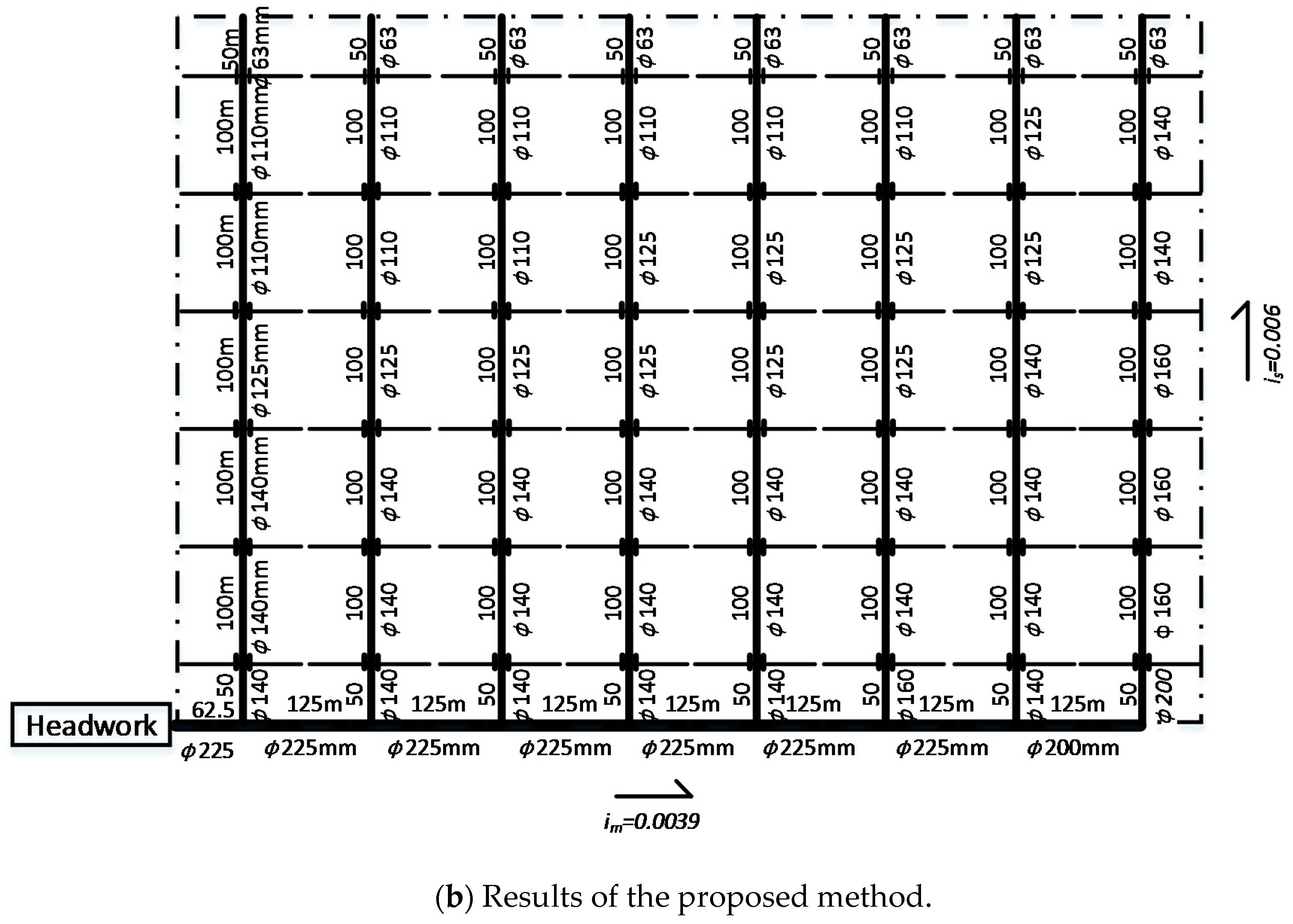
3.2. Optimization Results and Analysis

The layouts obtained for the MSMPN subsystem of the typical plot with the empirical method and the proposed method are displayed in Figure 9a,b, respectively.
The MSMPN subsystem of the scheme obtained with the empirical method consists of the main pipe and 10 sub-main pipes, whereas the MSMPN subsystem of the optimized scheme obtained with the proposed method comprises a main pipe and eight sub-main pipes. The number of branch pipes on each sub-main pipe is 12 for both the schemes. The pipe diameters obtained for the MSMPN subsystem with the empirical method are larger than those obtained for the MSMPN subsystem with our proposed method in most pipe sections.
The design results for the typical BLPN subsystem with the proposed and empirical methods are presented in Table 2. The empirical method generally does not segment the pipeline for optimization. It only designs a pipe diameter satisfying the requirement by using some empirical formulas according to the total discharge and pressure in the branch pipe. But the branch pipe is a porous outflow pipe during operation, and its discharge decreases on being gradually diverted. Thus, its diameter should decrease with discharge distribution. The proposed method anticipates this. Although the total length of the designed branch pipe in both methods was 62.5 m, the branch pipe obtained with the presented method consisted of three sections. Section 1 and Section 2 have a smaller diameter than that obtained with the empirical method. The diameter values are reasonable for reducing the cost of the pipes.
The value of the optimized Rdis was 0.3, which means the pressure head at the entrance of the BLPN subsystem accounts for thirty percent of the pressure head at the headwork, whereas the empirical method does not optimize Rdis and just use an empirical value of 0.45.
The total costs of the pipes in the WPN system scheme obtained with the proposed and empirical methods were 409, 454, and 564,901 Yuan, respectively. The total cost achieved with the proposed method was 27.5% lower than that achieved with the empirical method. The reduction in cost may be related to the fact that the empirical method divides the pipe network layout and pipe diameter optimization into two steps. The optimization of the pipe network layout is considered as one step, and pipe diameter optimization is considered as the second step. Due to these disparate calculations, holistic integration of the system calculations cannot be achieved. Empirical methods are typically artificial trial methods that depend on the experience and professional knowledge of the designer. The scheme designed by the designer is usually only a relatively economical solution. Thus, the solution obtained is only one of the solutions meeting the requirements. Such schemes can seldom be globally optimal solutions. Moreover, the empirical method makes insufficient considerations of the changes in pipe diameter with discharge and pressure variance, which results in a single design for branch pipes and sub-main pipes. The proposed method successfully overcomes these shortcomings of the empirical method.

4. Discussion

Although this study presents a new method with effective and stable performance for a self-pressurized drip irrigation system, the research has many limitations. First, this research is mainly aimed at comb-shaped pipe network systems. Further study is warranted for other layout patterns. Second, the study mainly concentrates on the situation in which the headwork of the irrigation system is located at a corner of the field. Further studies should consider situations in which the headwork is located elsewhere in the field. The change in the headwork position has a limited effect on the BLPN subsystem; however, it affects the pressure of each node in the MSMPN subsystem. These changes, in turn, affect the selection of the pipe diameter. Third, the proposed optimization method is only applicable to uniform slopes along the length and width of the field. Further studies are required regarding the conditions of terrain fluctuations along the length and width of the field.
The design of any irrigation system must consider the scheme of rotational irrigation. This study assumes that up to two branch pipes exist on a sub-main pipe for simultaneous irrigation. If multiple sub-main pipes are working simultaneously, the adjacent sub-main pipes are assumed to work simultaneously. The problem of the random rotation irrigation scheme for sub-main pipes is relatively complex and requires further research. The proposed method can be used for reference in future research. Finally, the proposed optimization method can assist a designer in designing drip irrigation pipe network systems under the aforementioned conditions. Although the proposed method can theoretically provide approximate global optimal resolutions for designers, the method must be carefully examined, and appropriate modifications should be made on the basis of reality before utilization.

5. Conclusions

In this study, the synchronous optimization model is proposed for a self-pressurized drip irrigation network layout and pipe diameter determination. A GA based on the IFD method was adopted to solve the model. Nm, Ns, and Rdis were used as links to achieve a suitable combination of the MSMPN subsystems, BLPN subsystems, and WPN system in the simultaneous optimization process of the WPN system. In the process of optimization, many constraints were solved by scientific coding as well as the IFD method, successfully overcoming the problem of poor convergence and difficulty in obtaining the global optimal solution caused by penalty function method under numerous constraints.
A typical case study is conducted, which proves the effective performance of the proposed method. Using this method, designers can easily complete the layout determination and diameter selection of the main, sub-main, and branch pipes in the self-pressured drip irrigation system by providing only some basic information regarding the irrigation area, such as the field size, field slope, and crop to be planted. The proposed method is an easy, fast, robust, and practical method for the design and management of self-pressurized irrigation systems.

Author Contributions

X.-Y.M. and R.-H.Z. conceived and designed the experiments. W.-Q.H. and Z.-K.L. contributed engineering design materials and engineering experience. R.-H.Z. and X.-Y.M. established the optimization models and designed the solution algorithm. R.-H.Z. and X.-Y.M. analyzed the data. R.-H.Z. wrote the paper, and X.-Y.M. and W.-B.N. revised the paper.

Funding

This research was funded by the National Science and Technology Support Program of China, grant number 2015BAD24B02; the National Key RandD Program of China, grant number 2017YFC0403202; the Special Fund for Agro-scientific and Research in the Public Interest of China, grant number 201503124.

Conflicts of Interest

The authors declare no conflict of interest.

Abbreviations

Lf, WfField length and field width
lb_min, lb_maxMinimum and maximum allowable branch pipe lengths
ll_min, ll_maxMinimum and maximum allowable lateral pipe lengths
Nm_min, Nm_maxMinimum and maximum number of segments per the main pipe
Ns_min, Ns_maxMinimum and maximum number of segments per sub-main pipe
Nm, NsNumber of main, and sub-main pipe sections
RdisPressure distribution ratio of the BLPN subsystem pressure to the entire pressure to be distributed
Db_endEnd section of the branch pipe
α1, α2, α3Ratios of the length of same-diameter sections of a branch pipe to the unallocated length of the branch pipe
lb1, lb2, lb3, lb4, lbLengths of branch pipe sections 1, 2, 3, and 4, and length of the branch pipe
Db1, Db2, Db3, Db4, Db_entDiameters of branch pipe sections 1, 2, 3, and 4, and diameter of the entrance section of the branch pipe
Qb1, Qb2, Qb3, Qb4, QbDischarges of branch pipe sections 1, 2, 3, and 4, and discharge of the branch pipe
CBLTotal cost of the pipes in the BLPN subsystem
HBL_maxMaximum total water head loss in the BLPN subsystem
ls_sec, lm_secLengths of the main and sub-main pipe sections
Ds1, Ds2, …, DsNsDiameters of sub-main pipe sections 1, 2, ..., Ns
Dm1, Dm2, …, DmNmDiameters of sub-main pipe sections 1, 2, ..., Nm
CMSMTotal cost of the pipes in the MSMPN subsystem
HMSM_maxMaximum total water head loss in the MSMPN subsystem
Nm_WPN, Ns_WPNNumber of main and sub-main pipe sections of the optimal WPN system
lb1_WPN, lb2_WPN, lb3_WPN, lb4_WPN, lb_WPNLengths of branch pipe sections 1, 2, 3, and 4, and length of the branch pipe of the optimal WPN system
Db1_WPN, Db2_WPN, Db3_WPN, Db4_WPN, Db_ent_WPNDiameters of branch pipe sections 1, 2, 3, and 4, and diameter of the entrance section of the branch pipe of the optimal WPN system
Qb1_WPN, Qb2_WPN, Qb3_WPN, Qb4_WPN, Qb_WPNDischarges of branch pipe sections 1, 2, 3, and 4, and discharge of the branch pipe of the optimal WPN system
Ds1_WPN, Ds2_WPN, …, DsNs_WPNDiameters of sub-main pipe sections 1, 2, ..., Ns of the optimal WPN system
Dm1_WPN, Dm2_WPN, …, DmNm_WPNDiameters of sub-main pipe sections 1, 2, ..., Nm of the optimal WPN system
CBL_WPNTotal cost of the pipes in the BLPN subsystem of the optimal WPN system
CMSM_WPNTotal cost of the pipes in the MSMPN subsystem of the optimal WPN system
CWPNTotal cost of pipes in the optimal WPN system
HBL_maxMaximum total water head loss in the BLPN subsystem of the optimal WPN system
HMSM_maxMaximum total water head loss in the MSMPN subsystem of the optimal WPN system

References

  1. Tan, S.; Wang, Q.; Zhang, J.; Chen, Y.; Shan, Y.; Xu, D. Performance of AquaCrop model for cotton growth simulation under film-mulched drip irrigation in southern Xinjiang, China. Agric. Water Manag. 2018, 196, 99–113. [Google Scholar] [CrossRef]
  2. Kuang, W.; Gao, X.; Gui, D.; Tenuta, M.; Flaten, D.N.; Yin, M.; Zeng, F. Effects of fertilizer and irrigation management on nitrous oxide emission from cotton fields in an extremely arid region of northwestern China. Field Crop. Res. 2018, 229, 17–26. [Google Scholar] [CrossRef]
  3. Wang, H.; Wu, L.; Cheng, M.; Fan, J.; Zhang, F.; Zou, Y.; Chau, H.Y.; Gao, Z.; Wang, X. Coupling effects of water and fertilizer on yield, water and fertilizer use efficiency of drip-fertigated cotton in northern xinjiang, china. Field Crop. Res. 2018, 219, 169–179. [Google Scholar] [CrossRef]
  4. Baiamonte, G. Advances in designing drip irrigation laterals. Agric. Water Manag. 2018, 199, 157–174. [Google Scholar] [CrossRef] [Green Version]
  5. El-Hendawy, S.E.; Schmidhalter, U. Optimal coupling combinations between irrigation frequency and rate for drip-irrigated maize grown on sandy soil. Agric. Water Manag. 2010, 97, 439–448. [Google Scholar] [CrossRef]
  6. Zhou, L.; Feng, H.; Zhao, Y.; Qi, Z.; Zhang, T.; He, J.; Dyck, M. Drip irrigation lateral spacing and mulching affects the wetting pattern, shoot-root regulation, and yield of maize in a sand-layered soil. Agric. Water Manag. 2017, 184, 114–123. [Google Scholar] [CrossRef]
  7. Zhou, L.; He, J.; Qi, Z.; Dyck, M.; Zou, Y.; Zhang, T.; Feng, H. Effects of lateral spacing for drip irrigation and mulching on the distributions of soil water and nitrate, maize yield, and water use efficiency. Agric. Water Manag. 2018, 199, 190–200. [Google Scholar] [CrossRef]
  8. Chakraborty, D.; Nagarajan, S.; Aggarwal, P.; Gupta, V.K.; Tomar, R.K.; Garg, R.N.; Sahoo, R.N.; Sarkar, A.; Chopra, U.K.; Sarma, K.S.S.; et al. Effect of mulching on soil and plant water status, and the growth and yield of wheat (Triticum aestivum L.) in a semi-arid environment. Agric. Water Manag. 2008, 95, 1323–1334. [Google Scholar] [CrossRef]
  9. Erenstein, O. Crop residue mulching in tropical and semi-tropical countries: An evaluation of residue availability and other technological implications. Soil Tillage Res. 2002, 67, 115–133. [Google Scholar] [CrossRef]
  10. Vázquez, N.; Pardo, A.; Suso, M.L.; Quemada, M. Drainage and nitrate leaching under processing tomato growth with drip irrigation and plastic mulching. Agric. Ecosyst. Environ. 2006, 112, 313–323. [Google Scholar] [CrossRef]
  11. Zhang, G.; Liu, C.; Xiao, C.; Xie, R.; Ming, B.; Hou, P.; Liu, G.; Xu, W.; Shen, D.; Wang, K.; et al. Optimizing water use efficiency and economic return of super high yield spring maize under drip irrigation and plastic mulching in arid areas of China. Field Crop. Res. 2017, 211, 137–146. [Google Scholar] [CrossRef]
  12. Feike, T.; Khor, L.Y.; Mamitimin, Y.; Ha, N.; Li, L.; Abdusalih, N.; Xiao, H.; Doluschitz, R. Determinants of cotton farmers’ irrigation water management in arid northwestern china. Agric. Water Manag. 2017, 187, 1–10. [Google Scholar] [CrossRef]
  13. Tian, F.; Yang, P.; Hu, H.; Liu, H. Energy balance and canopy conductance for a cotton field under film mulched drip irrigation in an arid region of northwestern China. Agric. Water Manag. 2017, 179, 110–121. [Google Scholar] [CrossRef]
  14. Wang, R.; Kang, Y.; Wan, S. Effects of different drip irrigation regimes on saline–sodic soil nutrients and cotton yield in an arid region of Northwest China. Agric. Water Manag. 2015, 153, 1–8. [Google Scholar] [CrossRef] [Green Version]
  15. Giménez, J.L.; Calvet, J.-L.; Alonso, A. A Two-Level Dynamic Programming Method for the Optimal Design of Sewerage Networks. IFAC Proc. Vol. 1995, 28, 537–542. [Google Scholar] [CrossRef]
  16. Alperovits, E.; Shamir, U. Design of optimal water distribution systems. Water Resour. Res. 1977, 13, 885–900. [Google Scholar] [CrossRef]
  17. Theocharis, M.E.; Tzimopoulos, C.D.; Sakellariou-Makrantonaki, M.A.; Yannopoulos, S.I.; Meletiou, I.K. Comparative calculation of irrigation networks using Labye’s method, the linear programming method and a simplified nonlinear method. Math. Comput. Model. 2010, 51, 286–299. [Google Scholar] [CrossRef]
  18. Arai, Y.; Koizumi, A.; Inakazu, T.; Masuko, A.; Tamura, S. Optimized operation of water distribution system using multipurpose fuzzy LP model. Water Sci. Technol.-Water Supply 2013, 13, 66–73. [Google Scholar] [CrossRef]
  19. Kirkpatrick, S.; Gelatt, C.D., Jr.; Vecchi, M.P. Optimization by Simulated Annealing. Science 1983, 220, 671–680. [Google Scholar] [CrossRef] [Green Version]
  20. Glover, F. Future paths for integer programming and links to artificial intelligence. Comput. Oper. Res. 1986, 13, 533–549. [Google Scholar] [CrossRef]
  21. Glover, F. Tabu search—Part I. ORSA J. Comput. 1989, 1, 89–98. [Google Scholar] [CrossRef]
  22. Glover, F. Tabu Search—Part II. ORSA J. Comput. 1990, 2, 4–32. [Google Scholar] [CrossRef]
  23. Goldberg, D.E. Genetic Algorithms in Search, Optimization & Machine Learning; Addison-Wesley: Reading, MA, USA, 1989. [Google Scholar]
  24. Kennedy, J.; Eberhart, R. Particle Swarm Optimization. In Proceedings of the IEEE International Conference on Neural Networks, IV, Perth, Western Australia, 27 November–1 December 1995; pp. 1942–1948. [Google Scholar]
  25. Dorigo, M.; Gambardella, L.M. Ant colony system: A cooperative learning approach to the traveling salesman problem. IEEE Trans. Evol. Comput. 1997, 1, 53–66. [Google Scholar] [CrossRef]
  26. Geem, Z.W.; Kim, J.H.; Loganathan, G.V. Harmony search optimization: Application to pipe network design. Int. J. Simul. Model. 2002, 22, 9. [Google Scholar] [CrossRef]
  27. Eusuff, M.; Lansey, K.; Pasha, F. Shuffled frog-leaping algorithm: A memetic meta-heuristic for discrete optimization. Eng. Optim. 2006, 38, 129–154. [Google Scholar] [CrossRef]
  28. Erchiqui, F. Application of genetic and simulated annealing algorithms for optimization of infrared heating stage in thermoforming process. Appl. Therm. Eng. 2018, 128, 1263–1272. [Google Scholar] [CrossRef]
  29. Keedwell, E.; Khu, S.T. A hybrid genetic algorithm for the design of water distribution networks. Eng. Appl. Artif. Intell. 2005, 18, 461–472. [Google Scholar] [CrossRef]
  30. Guerrero, M.; Montoya, F.G.; Baños, R.; Alcayde, A.; Gil, C. Adaptive community detection in complex networks using genetic algorithms. Neurocomputing 2017, 266, 101–113. [Google Scholar] [CrossRef]
  31. Kiziloz, H.E.; Dokeroglu, T. A robust and cooperative parallel tabu search algorithm for the maximum vertex weight clique problem. Comput. Ind. Eng. 2018, 118, 54–66. [Google Scholar] [CrossRef]
  32. Wang, Y.L.; Yu, Y.Y.; Li, K.; Zhao, X.G.; Guan, G. A human-computer cooperation improved ant colony optimization for ship pipe route design. Ocean Eng. 2018, 150, 12–20. [Google Scholar] [CrossRef]
  33. Dastmalchi, M.; Sheikhzadeh, G.A.; Arefmanesh, A. Optimization of micro-finned tubes in double pipe heat exchangers using particle swarm algorithm. Appl. Therm. Eng. 2017, 119, 1–9. [Google Scholar] [CrossRef]
  34. Simpson, A.; Dandy, G.; Murphy, L. Genetic algorithms compared to other techniques for pipe optimization. J. Water Resour. Plan. Manag. 1994, 120, 423–443. [Google Scholar] [CrossRef]
  35. Savic, D.A.; Walters, G.A. Genetic algorithms for least-cost design of water distribution networks. J. Water Resour. Plan. Manag. 1997, 123, 67–77. [Google Scholar] [CrossRef]
  36. da Conceição Cunha, M.; Sousa, J. Water distribution network design optimization: Simulated annealing approach. J. Water Resour. Plan. Manag. 1999, 125, 69–70. [Google Scholar]
  37. Chung, G.; Lansey, K. Application of the Shuffled Frog Leaping Algorithm for the Optimization of a General Large-Scale Water Supply System. Water Resour. Manag. 2008, 23, 797–823. [Google Scholar] [CrossRef]
  38. Trigueros, D.E.G.; Módenes, A.N.; Ravagnani, M.A.S.S.; Espinoza-Quiñones, F.R. Reuse water network synthesis by modified PSO approach. Chem. Eng. J. 2012, 183, 198–211. [Google Scholar] [CrossRef]
  39. Deb, K.; Pratap, A.; Agarwal, S.; Meyarivan, T. A fast and elitist multiobjective genetic algorithm: NSGA-II. IEEE Trans. Evol. Comput. 2002, 6, 182–197. [Google Scholar] [CrossRef] [Green Version]
  40. Ahn, C.W.; Ramakrishna, R.S. A genetic algorithm for shortest path routing problem and the sizing of populations. IEEE Trans. Evol. Comput. 2002, 6, 566–579. [Google Scholar] [Green Version]
  41. Michalewicz, Z.; Janikow, C.Z.; Krawczyk, J.B. A modified genetic algorithm for optimal control problems. Comput. Math. Appl. 1992, 23, 83–94. [Google Scholar] [CrossRef] [Green Version]
  42. Lavric, V.; Iancu, P.; Pleşu, V. Genetic algorithm optimisation of water consumption and wastewater network topology. J. Clean Prod. 2005, 13, 1405–1415. [Google Scholar] [CrossRef]
  43. Hartmann, S. A competitive genetic algorithm for resource-constrained project scheduling. Nav. Res. Logist. 2015, 45, 733–750. [Google Scholar] [CrossRef]
  44. Moradi, M.H.; Abedini, M. A combination of genetic algorithm and particle swarm optimization for optimal DG location and sizing in distribution systems. Int. J. Electr. Power Energy Syst. 2012, 34, 66–74. [Google Scholar] [CrossRef]
  45. Maity, S.; Roy, A.; Maiti, M. An imprecise Multi-Objective Genetic Algorithm for uncertain Constrained Multi-Objective Solid Travelling Salesman Problem. Expert Syst. Appl. 2016, 46, 196–223. [Google Scholar] [CrossRef]
  46. Giassi, M.; Göteman, M. Layout design of wave energy parks by a genetic algorithm. Ocean Eng. 2018, 154, 252–261. [Google Scholar] [CrossRef]
  47. De, M.; Das, B.; Maiti, M. Green logistics under imperfect production system: A Rough age based Multi-Objective Genetic Algorithm approach. Comput. Ind. Eng. 2018, 119, 100–113. [Google Scholar] [CrossRef]
  48. Babbar-Sebens, M.; Minsker, B.S. Interactive Genetic Algorithm with Mixed Initiative Interaction for multi-criteria ground water monitoring design. Appl. Soft. Comput. 2018, 12, 182–195. [Google Scholar] [CrossRef]
  49. Bi, W.; Dandy, G.C.; Maier, H.R. Improved genetic algorithm optimization of water distribution system design by incorporating domain knowledge. Environ. Model. Softw. 2015, 69, 370–381. [Google Scholar] [CrossRef]
  50. Michalewicz, Z. Genetic algorithms + data structures = evolution programs. Comput. Stat. Data Anal. 1996, 24, 372–373. [Google Scholar]
  51. Deb, K. An efficient constraint handling method for genetic algorithms. Comput. Meth. Appl. Mech. Eng. 2002, 186, 311–338. [Google Scholar] [CrossRef]
  52. Mu, S.M.S.; Su, H.S.H.; Mao, W.M.W.; Chen, Z.C.Z.; Chu, J.C.J. A new genetic algorithm to handle the constrained optimization problem. In Proceedings of the IEEE Conference on Decision & Control, Las Vegas, NV, USA, 10–13 December 2012. [Google Scholar]
Figure 1. Schematic of a self-pressurized drip irrigation network system.
Water 11 00489 g001
Figure 2. The grouping method of rotation irrigation of the two branch pipes working simultaneously.
Water 11 00489 g002
Figure 3. Flowchart of a genetic algorithm (GA) based on the IFD of the solution.
Water 11 00489 g003
Figure 4. Flowchart of the optimization.
Water 11 00489 g004
Figure 5. Sketch of a branch pipe.
Water 11 00489 g005
Figure 6. Code string for the optimization of the BLPN subsystem.
Water 11 00489 g006
Figure 7. Code string (chromosome) for the optimization of the MSMPN subsystem.
Water 11 00489 g007
Figure 8. Code string (chromosome) for WPN system optimization.
Water 11 00489 g008
Figure 9. Design results with the (a) empirical and (b) proposed methods.
Water 11 00489 g009aWater 11 00489 g009b
Table 1. Unit prices of different pipes.
Low-density polyethylene (LDPE) pipes (with a pressure capacity of 0.6 Mpa)
Outside diameter (mm)3240637590110125
Inner diameter (mm)28.835.255.46679.4100115
Unit price (Yuan/m)4.565.186.28.219.3610.2912.48
Unplasticized polyvinyl chloride (UPVC) pipes (with a pressure capacity of 0.6 Mpa)
Outside diameter (mm)637590110125140160
Inner diameter (mm)60.271.686105119.2132153
Unit price (Yuan/m)4.756.499.3312.4216.3720.3326.57
Outside diameter (mm)180200225250315355400
Inner diameter (mm)170190215240305345390
Unit price (Yuan/m)32.5140.3450.9363.5999.18119.97144.10
Table 2. Optimal design of the branch pipe of the typical BLPN subsystem.
Section NumberThe Proposed MethodThe Empirical Method
Length (m)Diameter (mm)Length (m)Diameter (mm)
1296362.590
21975
314.590

