Correlation Analysis Between Groundwater Decline Trend and Human-Induced Factors in Bashang Region


1
Faculty of Infrastructure Engineering, Dalian University of Technology, Dalian 116034, China
2
Department of Water Resources Research, China Institute of Water Resources and Hydropower Research, Beijing 100038, China
3
Information Center, Ministry of Water Resources, Beijing 100038, China
*
Author to whom correspondence should be addressed.
Water 2019, 11(3), 473; https://doi.org/10.3390/w11030473
Submission received: 18 January 2019
/
Revised: 24 February 2019
/
Accepted: 26 February 2019
/
Published: 6 March 2019
(This article belongs to the Section Hydrology)
Abstract
:In Northern China, many regions and cities are located in semi-arid regions, and groundwater is even the only source of water to support human survival and social development. Affected by human activities, the Bashang (BS) region (including Zhangjiakou City and part of Xilin Gol League) have showed a significant decline in groundwater levels in recent years. However, in the BS region, the causes for the decline in groundwater level were not clear. In this study, we used time series of multi-source data Moderate Resolution Imaging Spectroradiometer (MODIS), Gravity Recovery and Climate Experiment (GRACE) and Global Land Data Assimilation System (GLDAS) to analyze vegetation and groundwater changes based on linear regression models. The variation trends of NDVI (Normalized Difference Vegetation Index, derived from MODIS) and GWSA (groundwater storage anomaly, derived from GRACE and GLDAS) indicated the increasingly better vegetation in the agriculture planting areas, partially degraded vegetation in the grassland, and the declining groundwater level in the whole study region. In order to assess the impact of human-induced factors on vegetation and groundwater, the calculation model was proposed based on RUE (rain use efficiency) in this study. The calculation results showed that human-induced factors promoted the growth of vegetation in agricultural areas and accelerated the consumption of groundwater. In addition, we also obtained temporal and spatial distributions of human activities-affected regions. The area affected by human-induced factors in the south-central study area increased, which accelerated the decline in groundwater levels. From bulletin data, we found that the increasing tourists and vegetable production are respectively the most important factors for the increased consumption of urban water and agricultural water. Based on multi-source data, the influences of various human-induced factors on the ecological environment were explored and the area affected by human-induced factors was estimated. The results provide the valuable guidance for water resource management departments. In the BS region, it is necessary to regulate agricultural water use and strengthen residential water management.
1. Introduction
Groundwater is the world’s largest freshwater resource and plays a vital role in agricultural irrigation and food security [1]. Globally, groundwater accounts for one third of all freshwater withdrawals and supplies 42%, 36%, and 27% of water for irrigation, households and manufacturing, respectively [2]. In some regions, due to excessive dependence on groundwater resources, the rate of groundwater consumption increases and natural recharge is insufficient, thus eventually leading to a decline in groundwater levels [3]. This significant increase in groundwater consumption is common in arid and semi-arid regions because surface water resources are scarce in many arid regions and people can only support and expand agricultural production by pumping groundwater resources [1,3].
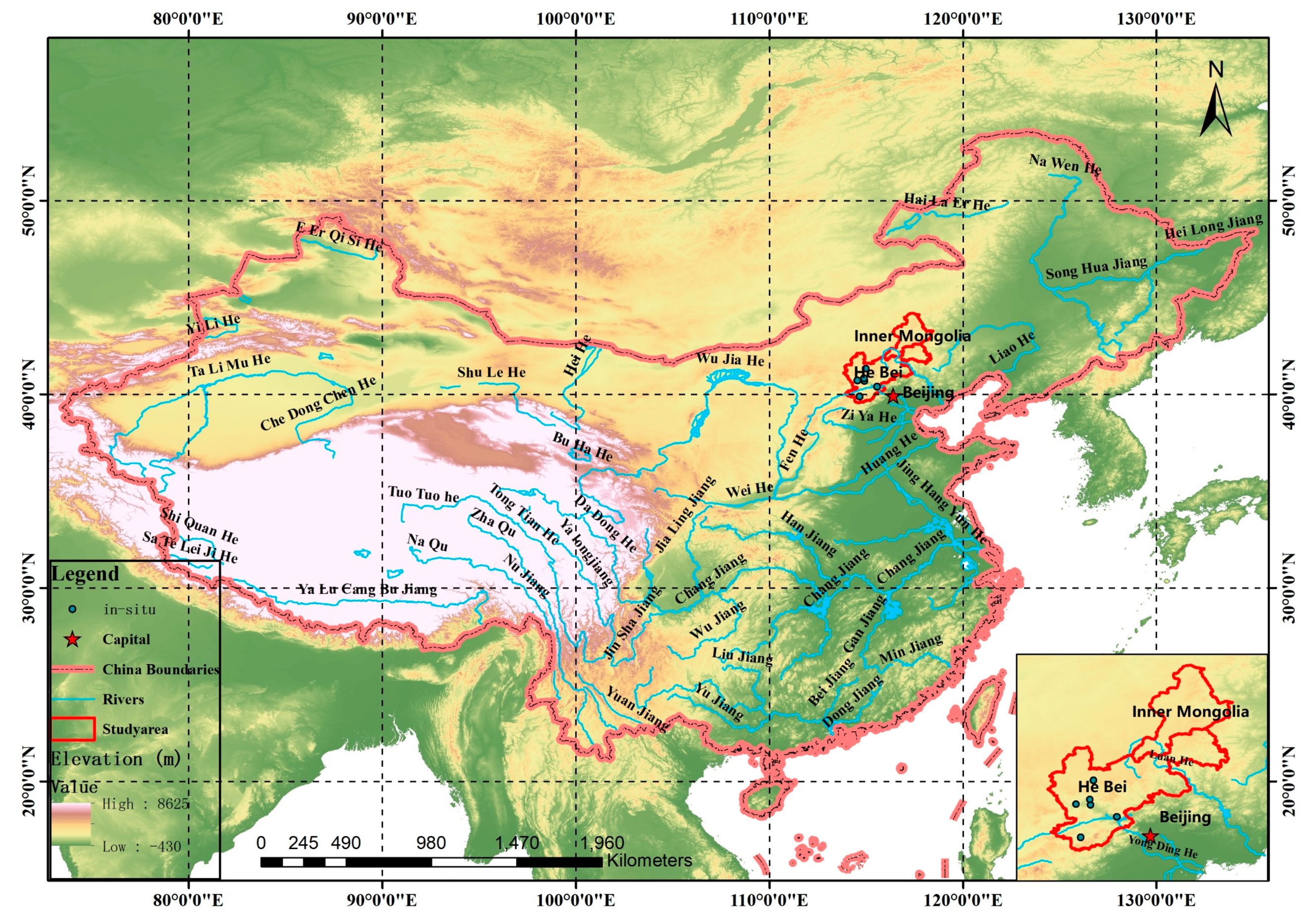
In recent years, in the northwestern part of China, except the Huang-Huai-Hai Plain, groundwater problems become more serious. The Bashang (BS) Region includes Zhangjiakou (ZJK) City and parts of Xilin Gol League in Inner Mongolia. The region is a typical rainfed agricultural area located in the agro-pastoral zone in Northern China (shown in Figure 1). Since the 20th century, the land uses in the BS region have been significantly changed. In the original landscape grasslands, food crops were planted and led to severe wind-induced soil degradation [4]. Due to the unique geographical location of ZJK, it is designed as a water conservation area of Beijing. However, ZJK is also an extremely water-deficient region [5]. At present, groundwater level in the BS is declining, although precipitation has increased in recent years. Some studies have identified that due to global warming, the temperature in Inner Mongolia has risen significantly, and the rising rate is 0.4 °C per decade [6,7]. As human activities and population increase, the shortage of water resources gradually becomes serious [5].
In the past few decades, groundwater in wide regions was depleted [8], such as Haihe Plain (HP). In the HP, about 53.7% of fresh water comes from groundwater. However, agricultural irrigation water mainly comes from groundwater, and partial groundwater comes from surface water, which is mainly supplied to urban citizen [9]. Due to long-term groundwater over-exploitation, shallow groundwater in some areas has disappeared and some problems such as land salinization and land subsidence occurred [10,11]. Climate change may directly affect the recharge of groundwater and indirectly affect the use of groundwater. Direct impact is the climate effect on reservoirs and fluxes and indirect effects are related to human activities [2,12,13]. As extreme weather events and population increase, various adverse environmental effects exacerbate groundwater depletion [14,15]. Timely monitoring of groundwater changes and human activities is of great significance for groundwater protection. However, due to the lack of groundwater level monitoring well in many regions, groundwater data often cannot achieve the required spatial resolution.
National Aeronautics and Space Administration (NASA) and the German Aerospace Center jointly developed the Gravity Recovery and Climate Experiment (GRACE) satellite mission provided a new opportunity to monitor groundwater storage variations from space [16,17]. Since the successful launch of the GRACE satellite in March 2002, more and more hydrologists have realized that it can be used as a new and effective tool to measure the changes in total terrestrial water storage (TWS) [18,19,20,21]. The groundwater storage change (GWSC) can be obtained by removing other components in the vertical direction of the terrestrial water storage change (TWSC), including soil moisture storage change (SMSC), surface water storage change (SWSC) and snow water equivalent change (SWEC) [22,23,24]. The hydrological water balance models can also be used to simulate the changes in global groundwater storage (GWS), but the accurate estimation of GWSC is still a challenge due to incomplete parameters [25]. Although land surface models (LSM) cannot simulate GWSC, they can predict the changes in soil moisture and water storage by simulating water and energy fluxes between the land surface and the atmosphere in general circulation models [26,27]. In earlier studies, Tapley et al. [28] and Chen et al. [29] indicated that the annual geoid variability observed by GRACE was consistent with the annual geoid variability simulated by Global Land Data Assimilation System (GLDAS). Subsequently, many regions with significant groundwater consumption in the world were explored, such as India [3,30,31], California’s Central Valley, USA [32,33], NCP (North China Plain) [11,34], and African [34,35,36]. In north of China, the loss trend of GWS was explored based on GRACE data. Feng et al. [11] estimated the rate of GWS depletion from 2003 to 2010 was −22 ± 3 mm in north of China (~370,000 km2). Huang et al. [34] divided the North China Plain into piedmont plain and east central plain and estimated the decline rates of the two regions from 2003 to 2013 to be −46.5 ± 6.8 mm/year and −16.9 ± 1.9 mm/year. Based on GRACE data, Zhong et al. [23] estimated the decreasing rate of GWS in the West Liaohe River Basin from 2005 to 2011 to be −0.92 ± 0.49 km3/year.
BS refers to the area formed by the sudden rise of the grassland. The general BS refers to the transition zone of Hebei Province to the Inner Mongolia Plateau, including the northern part of ZJK and some areas of Inner Mongolia (Figure 1), and the study area covers the entire BS and ZJK Region. From the south to the north, the study area shows the transition features (monsoon climate to continental climate; humid zone to semi-arid zone) and is more susceptible to natural disasters and human activities [37]. The study area is still a typical degraded ecosystem with increased human activities. In the northern part of the study area, as natural grassland was artificially cultivated, soil desertification intensified and many cultivated lands were abandoned by farmers. In the southern part of the study area, the groundwater level declined due to increased agricultural production activities. The main sources of shallow groundwater recharge in the BS region are precipitation and irrigation infiltration. This region belongs to endorheic rive hydrogeological unit and there is less groundwater interaction between study area and outside. Before 2000, the flow field of groundwater was in its natural state. After 2000, due to agricultural exploitation, it was accelerated and the groundwater flow field was changed. At present, groundwater discharge is mainly based on groundwater exploitation and evaporation [38]. Agricultural water consumption in ZJK accounted for 73.9% of the total water consumption in 2016 [5]. Therefore, it is necessary to conduct a more in-depth analysis on groundwater in the region.
Previous researches in the study area were seldom performed based on remote sensing and hydrological models, especially GRACE satellites. GRACE combined with GLDAS can provide stable and temporal-spatial continuous groundwater change datasets for the assessment of groundwater changes in regions without proper monitoring conditions. The study aims to the effects of vegetation and human activities on groundwater from remote sensing, LSM and in situ measurement data. The research route is shown in Figure 2. In the study, we estimated temporal and spatial variations of groundwater in the BS region by combining multi-source data from 2003–2016, assessed the causes for groundwater decline, analyzed the impact of different factors on groundwater changes, and gave management advices. Most importantly, we modified RUE (rain use efficiency) model and verified that it was applicable to explore groundwater in agricultural regions with frequent human activities.
2. Methods and Materials
2.1. Groundwater Decline Assessment Method
As described in Section 1, GWSC can be obtained by subtracting the variation of other components, including SMSC, SWSC, and SWESC, from TWSC. Similarly, groundwater storage anomalies (GWSA) can also be obtained by subtracting the anomalies of other components from TWSA (unit is centimeter), i.e., soil moisture storage anomalies (SMSA), surface water storage anomalies (SWSA) and snow water equivalents anomalies (SWESA) [39]:
GWSA = TWSA – SMSA – SWSA – SWESA.
In the study area, SWSA is small and not considered in the calculation of GWSA. In Equation (1), SMSA and SWESA used to derive the GWSA were estimated with four different versions of GLDAS LSMs, including CLM, MOSAIC, NOAH, and VIC [40,41,42,43]. Many researchers showed that the changes in groundwater storage could be successfully separated from GRACE data and that the output of GLDAS LSMs provided the SMSA and SWESA variables in Equation (1) [32,44]. In addition to GRACE and GLDAS data to estimate groundwater trends, in-situ measurement groundwater level data is used to validate groundwater trends.
2.2. Assessment Method of Human-Induced Factors
Rain use efficiency was the ratio of aboveground net primary production (ANPP) to annual precipitation in previous studies and was used to assess land degradation or improvement in arid and semi-arid areas [45,46]. Wessels et al. [47] compared the relationship between satellite-derived NPP divided by rainfall and annual NDVI divided by rainfall for every pixel and indicated that the vegetation production was correlated with rainfall in most parts of South Africa. Other researchers also found the relationship between NDVI and NPP in other study areas [48,49,50]. Therefore, to further explore the causes for land degradation, we can differentiate the effects of precipitation and human-induced factors on vegetation based on NDVI and precipitation data. In the theoretical basis of RUE, it is assumed that the relationship between NDVI and precipitation is nearly a linear relationship. However, in the practical study, the intercept of the regression line is not zero. Some studies identified that the NDVI of the irrigated area was larger than zero even when the precipitation was close to zero [51]. If RUE is simply considered to be the ratio of NDVI to precipitation, then RUE depends on precipitation and decreases with the increase in precipitation.
In arid and semi-arid regions, NDVI has a strong linear relationship with precipitation [52]. In addition to climate effects, the effects of human-induced factors are also important [45,47]. The effects of precipitation and human factors on NDVI (in pixel scale) can be quantified as:
where NDVI is the annual mean MODIS NDVI; is annual accumulated precipitation; a and b are the slope and intercept of the regression line, respectively; is the change of vegetation caused by human activities. If the vegetation in the study area is changed due to the influence of human factors such as returning farmland to forests and planting structure changes, the value of is not zero. Zhang et al. [53] modified the before calculating the RUE in order to more clearly monitor land degradation or improvement in Badain Jaran Desert (BJD). In this study, we calculated the RUE according to the method proposed by Zhang et al. [53]. We assumed that the human activities from 2003 to 2009 were stable. The pixel-by-pixel ordinary least squares regression was performed with the NDVI and the precipitation and the intercept b of the stable human activity period was obtained. RUE based on human activity stabilization period modification is defined as:
The trend in the study area is stable, indicating that human activities in the region remain stable or do not happen; if the RUE trend in the study area is changed, human activities in the region promote vegetation growth, 10,000 was used here to enlarge the value.
Due to the different types of vegetation cover in the study area, this method shows some defects in the application in the BS region. The BS region has more precipitation and crops than the BJD Region and groundwater irrigation is more important for vegetation growth. In the study area, the effects of adequate precipitation and precipitation shortage on vegetation should be considered at the same time. If human activities are assumed to be stable in earlier years, irrigation activities carried out due to insufficient precipitation may be ignored in growth seasons. Based on the monthly data, we accumulated the precipitation and NDVI for each season separately and analyzed the spatial distribution of precipitation and NDVI in different years. With the season division method, we can obtain the maximum NDVI and precipitation and minimum NDVI and precipitation in the same season in different years. In the agricultural area, if there is sufficient precipitation, there is less irrigation and the NDVI characteristics of the vegetation are obvious. In contrast, if there is insufficient precipitation, irrigation is required to ensure vegetation growth. The study was mainly performed in the Q2nd (Mar, Apr, and May) and Q3rd (June, July, and Aug) because the average temperatures in the Q1th (Dec, Jan, and Feb) and Q4th (Sep, Oct, and Nov) were below zero and vegetation stopped growth. In the study area, irrigation mainly occurs in the season when the hydrothermal conditions are not qualified, so the divided season can highlight the influence of human activities. Chen et al. [54] proposed a fuzzy pattern recognition method to evaluate the vulnerability of groundwater and calculated different types of evaluation factors for membership degree. In this study, membership degree equation is used to calculate the membership degree of precipitation and NDVI in time series. The membership degree can be calculated as follows:
where is the pixel in the precipitation or NDVI images; i and j respectively represent rows and columns; represents the maximum value of the (i, j) pixel in the entire time series (y) images (precipitation or NDVI); represents the minimum value of the (i, j) pixel in the entire time series (y) images (precipitation or NDVI); is the membership degree of the current time image (i, j) pixel for the maximum and minimum values.
The membership degrees of each pixel in the precipitation and NDVI time series images were respectively calculated with Equation (5). Based on the calculation results of the membership degrees of precipitation and NDVI, the impact of human activities on vegetation can be evaluated with the RUE equation below:
where indicates the extent to which human-induced factors affect vegetation growth on each pixel and also reflect the spatial and temporal distributions of human activities; is in NDVI images; is in precipitation images. If the value of is less than 1, the precipitation can satisfy the vegetation growth and there is no significant human-induced factors promoting the vegetation growth; if the value of is higher than 1, the precipitation cannot satisfy the vegetation growth and there is significant human-induced factors promoting the vegetation growth. If the value of is equal to 1, it indicates that the precipitation reaches the critical point required for vegetation growth. The higher the value of is, the higher the probability that the vegetation of the pixel is affected by human-induced factors is.
2.3. Statistical Methods
This paper introduced a linear regression model to examine the temporal trend in the NDVI dataset with time as an independent variable and NDVI as a dependent variable. The correlation coefficient (r values) and slope of the model output represent the strength and magnitude of the calculated trend [55,56]. The equations of slope and r values are expressed as follows:
where Slope is the change slope; i is the time corresponding to variable X and N is the quantity of the samples.
where is the covariance of the variable X and the variable Y; is the variance of X; is the variance of Y.
In this study, the significance level of the time series linear trends of different elements was detected based on the Mann–Kendall trend test.
2.4. Data Collection
2.4.1. Normalized Difference Vegetation Index
Currently, Normalized Difference Vegetation Index (NDVI) has been widely used to monitor vegetation changes at different scales [57,58,59,60]. It is defined as:
where NIR and RED respectively represent near-infrared (~0.860 μm) and red (~0.660 μm) surface reflectance.
The Moderate Resolution Imaging Spectroradiometer (MODIS) Vegetation Index (NDVI) product has a variety of spatio-temporal resolutions: spatial resolutions of 250 m, 500 m, and 1000 m, and temporal resolutions of 16 days and one month. This paper selects MOD13A3 with a spatial resolution of 1000 m at a monthly time scale. The product can be obtained from multiple sources such as Data pool, NASA Earthdata search and Earth Explorer. Due to the influences of clouds and snow, the data of some winter months were not complete. We used the linear interpolation method to gap-fill the missing data. In order to explore the trend of NDVI in the study area, the annual mean NDVI data were obtained from the monthly NDVI.
2.4.2. Precipitation
Monthly precipitation gridded products were provided by the National Meteorological Information Center [23,53]. This data is based on the precipitation data of 2472 stations on the ground in China. The space interpolation was performed by Thin Plate Spline, and the monthly Chinese precipitation data (unit is millimeter) of 0.5° × 0.5° from 2003 to 2016 were obtained. Since the spatial resolution of the MODIS NDVI data used in this paper was 1 km×1 km, which did not match the 0.5-degree requirement of the precipitation data, the adopted resampling method should ensure that the precipitation data was consistent with the spatial resolution of the NDVI data.
2.4.3. Groundwater Storage Anomalies Derived from GRACE Data
Currently, there are three official agencies that offer GRACE data products: the Center for Space Research (CSR) in Austin, the GeoForschungs Zentrum (GFZ) in Potsdam and the Jet Propulsion Laboratory (JPL) in Pasadena [22]. In the above three research centers, CSR and JPL provide GRACE data products respectively for two different methods, spherical harmonics (SH) and mascon solutions, whereas GFZ only provides SH method products. The GRACE SH and mascon solution products were based on the same GRACE Level-1 observations and time-mean baseline and both of them used C20 [61], degree-1 coefficient corrections [62] and glacial isostatic adjustment (GIA) [63]. Unlike mascon products, SH products need to remove north-south stripes and use Gaussian smoothing to remove high-frequency noise in the SH coefficients [64]. The mascon products provided by CSR and JPL were used in this study because mascon products had the higher resolution (0.5° × 0.5°) and the better S/N ratios of mascon fields. Compared with traditional SH products, the results of the mascon products are directly derived from the original GRACE data and are not processed by empirical filtering. However, mascon products can provide TWSA estimates comparable to SH products [65,66]. CSR mascon products (RL05_Mascons_v01) differ from JPL mascon products (RL05M_1. MSCNv02) since JPL needs to apply mascon-set of 0.5-degree gain factors. The gain factor is a multiplication factor that minimizes the difference between the smooth and unfiltered monthly water storage changes and land hydrology of the model at any geographic location [67]. The JPL mascon product and gain factor are calculated as follows:
where x is longitude index; y is latitude index; t is time (month) index; s(x,y) is the scaling grid.
TWSA’(x,y,t) = TWSA(x,y,t) × s(x,y),
Since early 2011, partial GRACE time series data are lost every year for the effective battery management of the satellite. The linear interpolation method used in the previous study [68] was used to obtain the CSR and JPL mascon data sets of continuous time-series.
2.4.4. Global Land Data Assimilation Systems (GLDAS)
GLDAS was jointly developed by scientists from multiple institutions, including National Aeronautics and Space Administration (NASA), Goddard Space Flight Center (GSFC), National Oceanic and Atmospheric Administration (NOAA), and National Centers for Environmental Prediction (NCEP) [27]. GLDAS is a global, high-resolution, off-line ground model system that combines satellite data with ground monitoring data to produce optimal fields of land surface states and fluxes in near-real time. GLDAS LSMs overcome the data loss in monitoring sites missing lands and provides time-continuous datasets [69,70]. The temporal resolution of 4 LSMs used in this study was a month and the spatial resolution was 1° × 1°. Model characteristics determine the number of vertical levels of soil moisture. Soil depths (layers) in CLM, MOSAIC, NOAH, and VIC are 3.43 m (10 layers), 3.50 m (3 layers), 2.0 m (4 layers), and 1.9 m (3 layers), respectively. The SWS and SWES produced by GLDAS LSMs are state variables and need to be processed with the same time-mean baseline as the GRACE data [24]. To get better results, like some of the previous researchers, we used the aggregated values of SMSA and SWESA produced by the four LSMs models as the other components of the TWSA subtraction.
2.4.5. In-Situ Measurement Data
From Groundwater Level Yearbook released by China Institute of Geological Environment Monitoring (CIGEM) [71], groundwater monitoring well observation data were obtained. However, the collected time series of groundwater level data were not continuous data (Figure 3b). In order to compare the trend between GWSA-derived GRACE data and groundwater level data, it is necessary to convert the groundwater level data. GWSA data baseline is from 2004 to 2009 and the groundwater level data also need to be converted into groundwater level anomalies (GWLA) by using the same processing method.
2.4.6. Statistical Bulletin Data
In the past ten years, human activities in the BS region changed significantly due to the expansion of agriculture and the increasing population. The Statistics Bureau of ZJK and BS released statistical bulletins on national economic and social development every year since 2006. At the same time, the Water Resources Bulletin data (from 2003 to 2016) were also collected [72]. Agricultural planting structure changes and population changes data were obtained from the statistical bulletins. The main data of agricultural planting structure changes include the data of food (low water consumption) production and vegetable (high water consumption) production. It is worth noting that the population information obtained by ZJK and Xilin Gol League mainly includes resident population and floating population. In recent years, with the rapid development of tourism, the number of floating populations has increased significantly, whereas the resident population has not changed significantly.
2.5. Uncertainty Analysis
At present, uncertainties exist in different GRACE products due to different processing methods of GRACE data. Landerer and Swenson [73] provide gridded leakage and GRACE measurement error fields, thus allowing users to strictly estimate the TWS uncertainty in the study area. Scanlon et al. [74] selected 176 river basins as the study area and found that CSR-M, JPL-M, and CSR Tellus gridded spherical harmonics rescaled (sf) (CSRT-GSH.sf) had the high correlation. In addition, the uncertainty of the three data products was also estimated. Wiese et al. [67] discussed the post-treatment of the JPL RL05M GRACE mascon solution to reduce the leakage errors introduced by the land/ocean boundaries and the leakage errors introduced by the mascon solution.
In this study, the uncertainty of the TWSA derived from CSR-M was obtained by calculating the residual. In the calculation of this residual, it is necessary to remove long-term trends and interannual, annual, and semi-annual amplitudes from original signals. The 13-month moving average method can be used to eliminate interannual signals. The root mean square of the residual was used to indicate the uncertainty of the TWSA.
In the uncertainty estimation of TWSA derived from JPL-M, it is necessary to consider both leakage and GRACE measurement errors. The uncertainty of the measurement has been given on the website and the uncertainty of the measurement is given by the diagonal elements from the posteriori covariance matrix from the gravity inversion. Wiese et al. [67] calculated the leakage error of 176 basins by using a synthetic simulation.
In GWSA calculation, it is necessary to remove GLDAS surface water storage anomalies (SMSA + SWESA) from GRACE-derived TWSA. The uncertainty in GLDAS surface water storage anomalies was estimated based on the standard deviation of the time series of four GLDAS models (Common Land Model (CLM), MOSAIC, NOAH and Variable Infiltration Capacity (VIC)).
3. Results
3.1. TWSA and GWSA from 2003 to 2016
Figure 3 shows the results of the TWSA and GWSA time series in the study area. Figure 3a shows the monthly TWSA (derived from CSR and JPL) and yearly precipitation (PRE) from 2003 to 2016 and the shadow indicates the uncertainty of CSR-derived TWSA (±1.96 cm) and JPL-derived TWSA (±2.31 cm), respectively. Before 2009, low precipitation did not result in a larger amplitude of the TWSA. However, the TWSA in 2009 and 2011 declined significantly in the case of low precipitation. After 2014, although the amount of precipitation increased, the TWSA declined more significantly. From the perspective of time series, the decline trend of TWS in the BS region is not obvious. Compared to the years before 2009, the amplitude of TWSA increased after 2014.
Figure 3b shows the time series of GWSA derived from GRACE and GLDAS. The grey line represents the GWSA obtained by removing surface water storage anomalies (SMSA + SWESA) simulated by different models (CLM, MOSAIC, NOAH, and VIC) from TWSA. The blue line and the red line are the mean values of the GWSA calculated by the TWSA provided by CSR and JPL and the four models, respectively. After removing surface water from TWSA, the GWSA time series showed a significant declining trend, especially after 2013. During the whole study period from 2003 to 2016, the declining rate of GWSA derived from GRACE and GLDAS were −0.44 ± 0.18 cm/year (CSR) and −0.37 ± 0.15 cm/year (JPL), respectively. Less precipitation in 2009 and 2011 caused a significant decline in GWSA, but precipitation in 2010 and 2012 allowed GWSA to recover a stable level in previous years. From the beginning of 2014 to the end of 2016, some worrying results were observed. The declining rate of GWSA increased, although the increased precipitation effectively promoted the recovery of GWSA, which did not stabilize the GWSA amplitude.
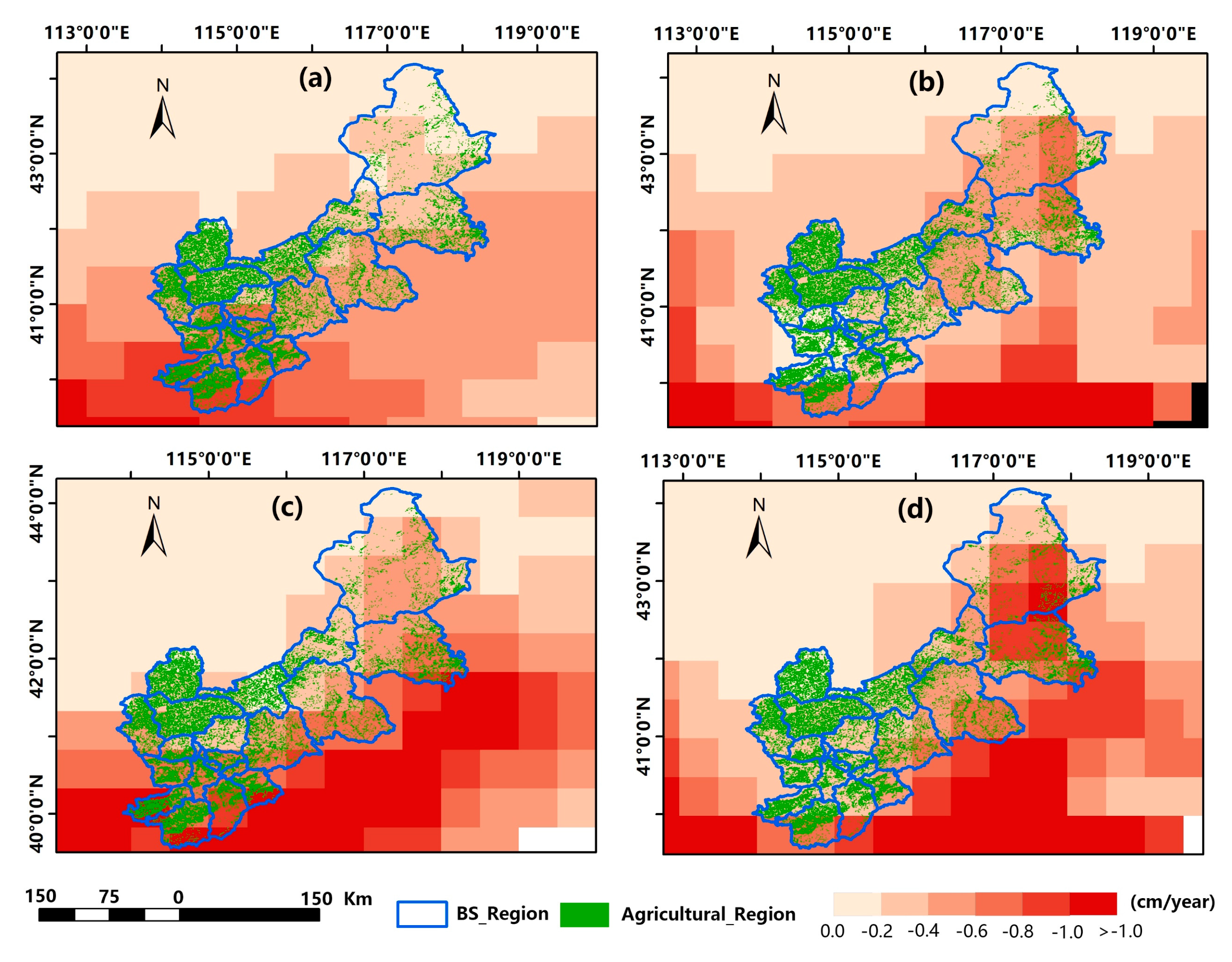
In order to obtain the spatial distributions of the TWSA and GWSA annual trends, the slope method was used to calculate the trend of each pixel in the GRACE images. The central and southern TWSA declined significantly in the study area (Figure 4a) and TWSA declined significantly in eastern and central parts of the study area (Figure 4b). After removing surface water in the GLDAS model from the GRACE data, the CSR-derived GWSA and the JPL-derived GWSA showed the consistent declining trend, indicating that the groundwater decline rate in the southern part of the study area was higher than that in the north.
3.2. Vegetation Changes in the Study Area
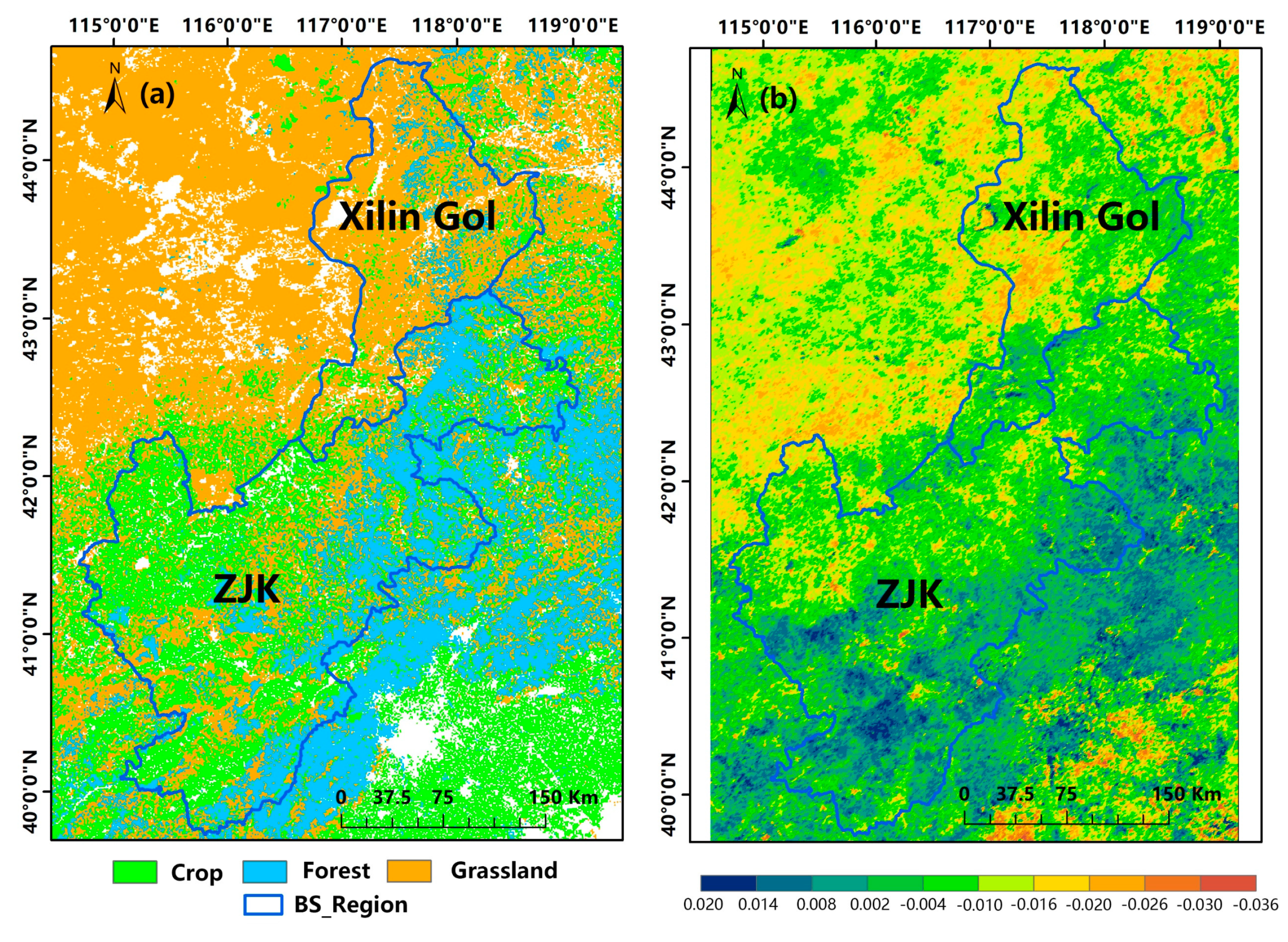
Figure 5a shows the land cover in the study area in 2015 and Figure 5b shows the trend of the NDVI (from 2003 to 2016). In Xilin Gol, the NDVI of the grasslands in the western region showed a declining trend and the NDVI in the southern agro-pastoral zone showed an increasing trend. However, ZJK showed an overall growth trend of NDVI except the northwest. The increasing trend of NDVI was more obvious in the southern region. In ZJK, the NDVI in the agricultural area and the forest region showed an increasing trend (Figure 5a).
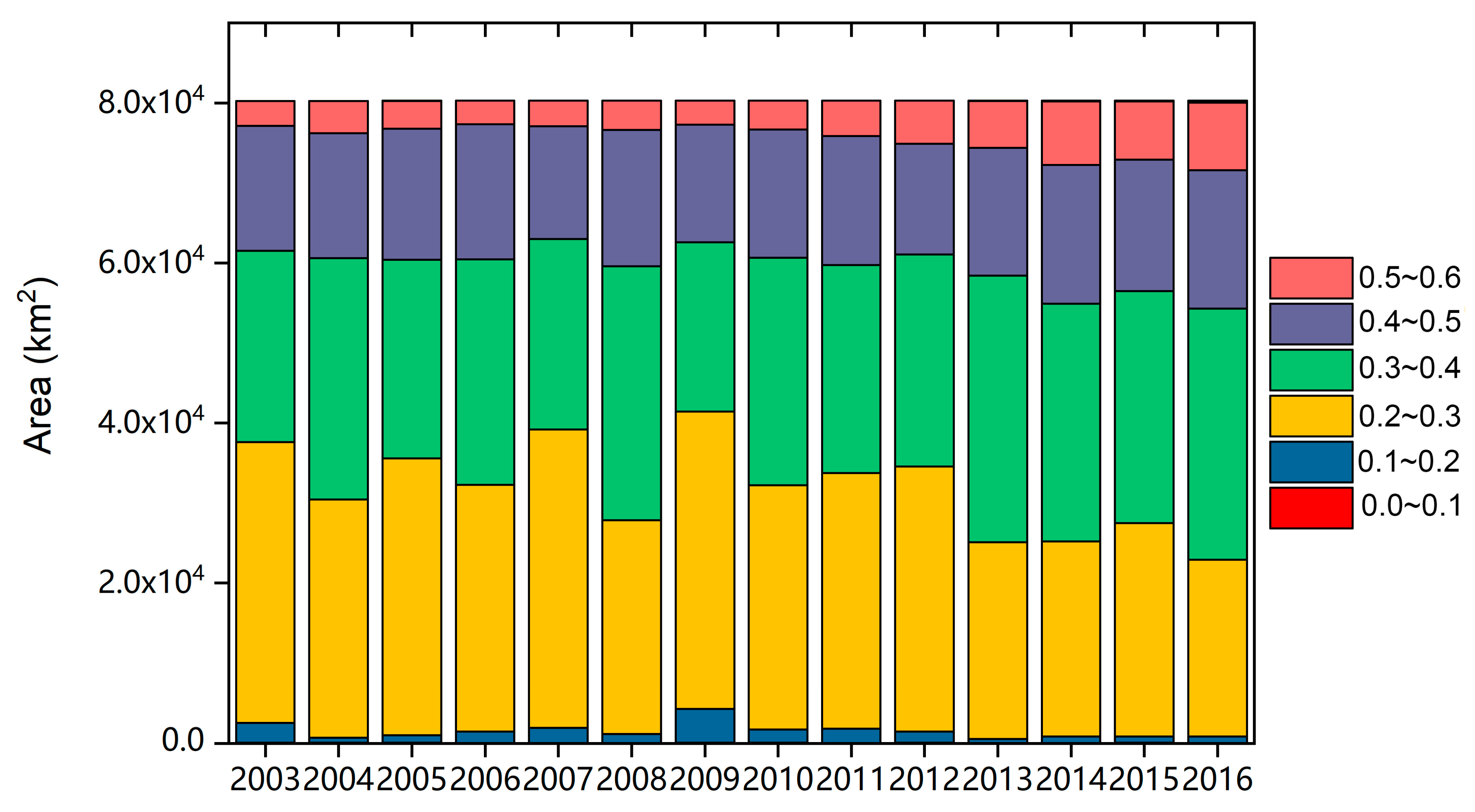
After dividing the value range of NDVI, the number of NDVI pixels with different interval values can be obtained to more directly indicate the change of time series NDVI (Figure 6). Before 2010, the number of pixels in the NDVI high-value interval (0.4~0.6) was stable, whereas the number of pixels in the NDVI interval of 0.2 to 0.4 varied greatly. After 2010, the number of pixels in the NDVI high-value interval (0.4~0.6) increased significantly. Especially after 2012, the number of pixels in the NDVI median-value interval (0.2~0.4) also increased significantly and was stabilized. The annual precipitation data of the time series indicated that the precipitations in 2007, 2009, and 2011 were lower than the annual average. However, the vegetation growth in 2011 was better than that in 2007 and 2009 and the vegetation growth in 2007 and 2009 was basically the same. Naturally, vegetation growth under the same precipitation conditions should be similar. In 2011, human activities (irrigation, reclamation, and crop pattern change) significantly promoted vegetation growth.
3.3. Calculation Results in the BS Region
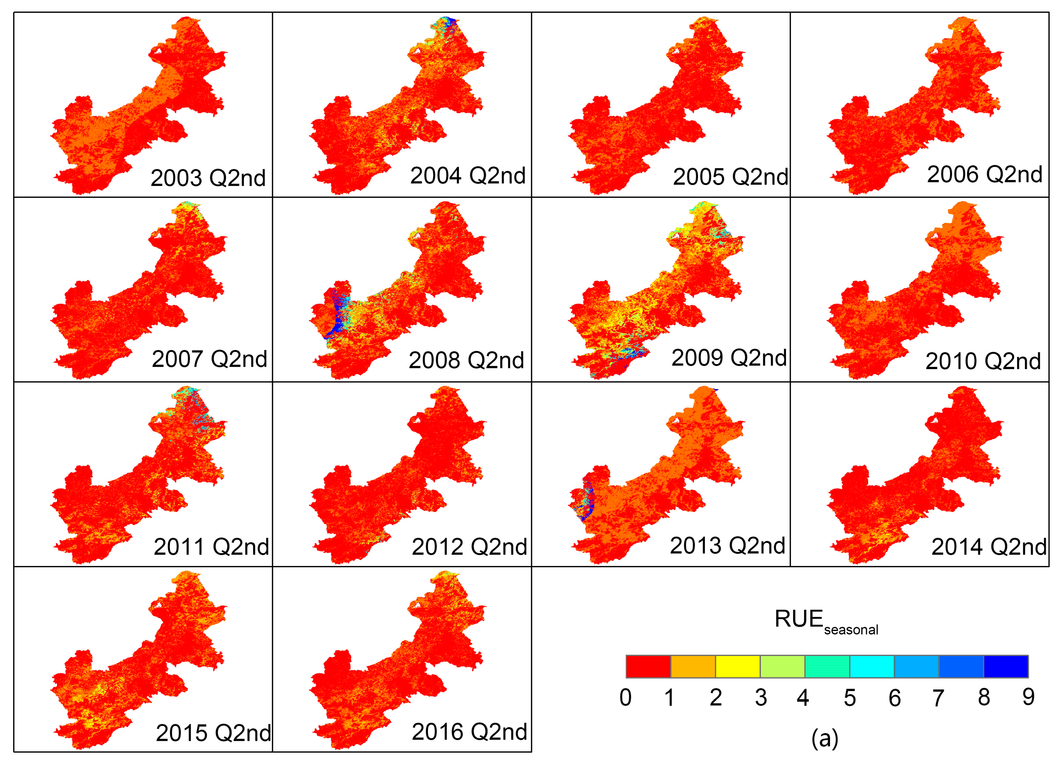
Before 2010, human-induced factors in 2004, 2008 and 2009 showed the most significant influences on vegetation growth (Figure 7a). In Q2nd of 2004, human-induced factors in the northern region promoted vegetation growth obviously. Human-induced factors promoted vegetation growth in the southern part of the study area in 2008 Q2nd and in 2009 Q2nd, vegetation growth in the entire study area was affected by human-induced factors. After 2010, except that vegetation growth in the smaller area was affected by human-induced factors in Q2nd of 2012, human-induced factors showed significant influences on vegetation growth in other years. The precipitations in Q2nd of 2011 and Q2nd of 2013 were respectively 46.31 mm and 31.82 mm, which were significantly lower than those in the same period of the entire time series. The area influenced by human-induced factors in Q2nd of 2013 was larger than that in Q2nd of 2011 due to better vegetation growth in Q2nd of 2013. In recent years, the areas affected by human-induced factors in Q2nd were more concentrated in the central and southern regions.
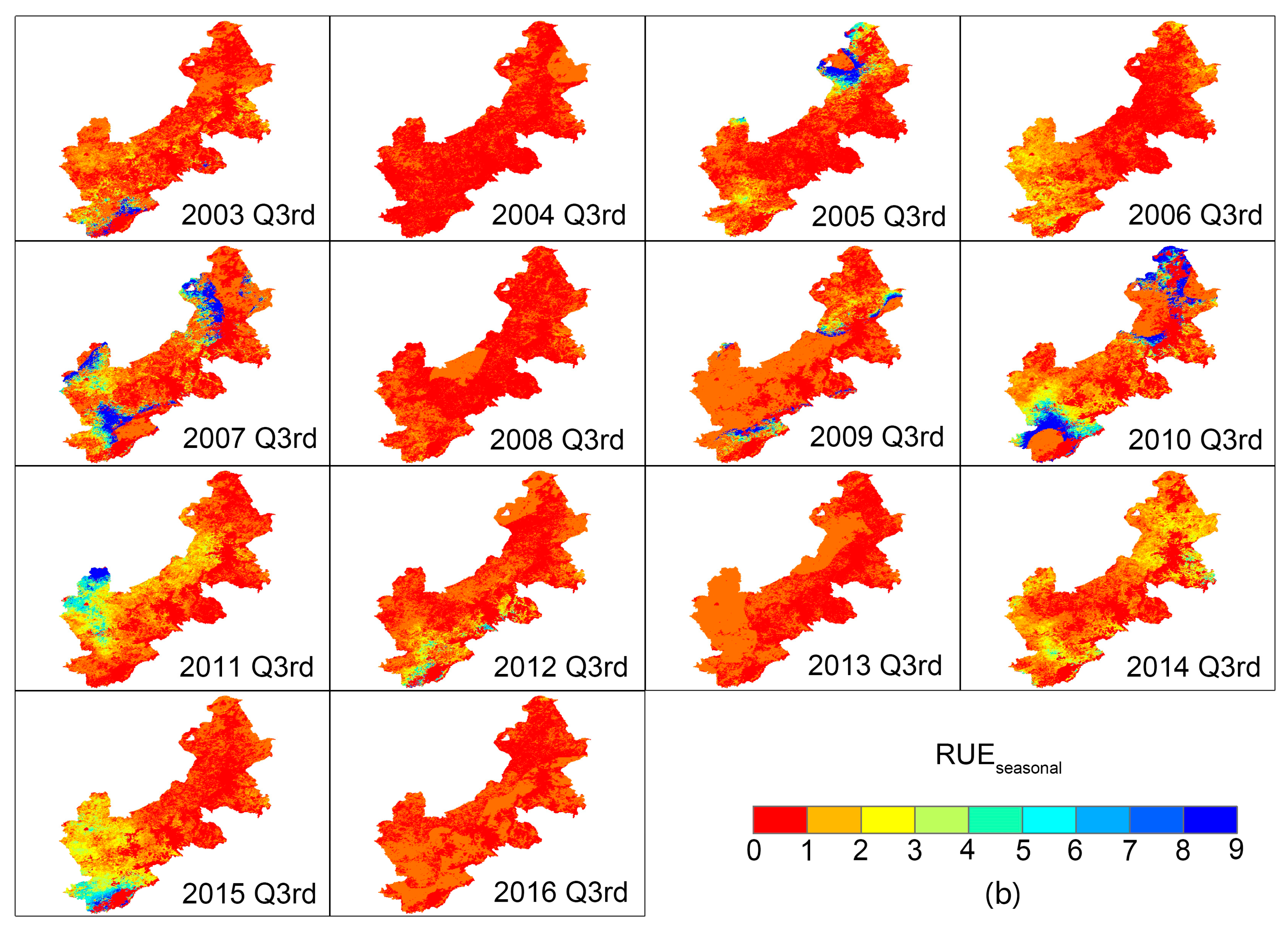
In Figure 7b, the calculation result of Q3rd shows a larger variation than that in Q2nd due to the unbalanced precipitation and more significant vegetation characteristics in every year of the time series. There is also a significant difference in annual precipitation among different years. In the calculation results of Q3rd, the influences of human-induced factors on vegetation growth were not significant in 2004, 2008, 2013, and 2016. We found that the precipitation in Q3rd was similar in 2003, 2005, 2011, 2014, and 2015 (between 210 mm and 230 mm), but their NDVI were different, as observed in the results. The calculation results of in both Q3rd and Q2nd indicated that the influences of human-induced factors in the southern region of the study area were more significant than those in the north. The difference was consistent with the analysis results of NDVI trend.
We divided the study area into three sub-regions (Region A, Region B and Region C) to statistically analyze the relationship between human-induced factors and groundwater changes (Figure 8). Region A is the Xilin Gol (mainly covered by grasses); Region B is the eastern part of the study area (mainly covered by forests and crops); Region C is the central and western regions of the study area (mainly covered by crops and forests). In time series of Region A in Q2nd and Q3rd, NDVI or precipitation showed no significant upward and downward trends. The NDVI of Region B and Region C showed a clear upward trend during Q2nd and Q3rd and the precipitation of Region C in Q2nd showed downward trend.
The results indicated the degree of mismatch between precipitation and NDVI, and the number of pixels with value greater than 1 in the statistical region could represent the influencing degree of human-induced factors in the region. Due to the small area of the Region B, it is not suitable to independently analyze the GWSA. In this paper, a combined analysis of GWSA was performed for Region A and Region B. In Region A, the relationship between and GWSA in Q2nd and Q3rd was not clear. The influence of human-induced factors on vegetation was not the main reason for groundwater reduction. In Region B and Region C, the time series of was negatively correlated with the time series of GWSA (CSR and JPL) in Q3rd. This indicated that the human-induced factor that had a greater impact on vegetation in these regions was groundwater irrigation. For the same Region A and Region B of GWSA, the reason for the decline in groundwater level in these regions is more likely to be vegetation irrigation in Region B. In the Q2nd in Region C, the growth characteristics of crops were not obvious due to low temperature. Conversely, Region B had the more significant vegetation growth characteristics in the Q2nd due to the large forest area. The crop growth characteristics of the Q2nd were not significant and there was no significant change in the calculation results of . In the Q3rd, the area affected by human-induced factors in Region B and Region C showed a significant increase trend. Especially after 2010, the average area affected by human-induced factors was significantly higher than that in the period from 2003 to 2010. These results indicated that in Region B and Region C, the area affected by human-induced factors in the Q3rd was getting larger and larger, thus accelerating the decline of groundwater level. Although the area affected by human factors was not significantly correlated with the decline of groundwater level in Q2nd (Figure 8b), the decline in groundwater level might be caused by irrigation. Less precipitation did not guarantee the consumption of vegetation during the germination period, especially in 2015.
3.4. Statistical Results of Bulletin Data
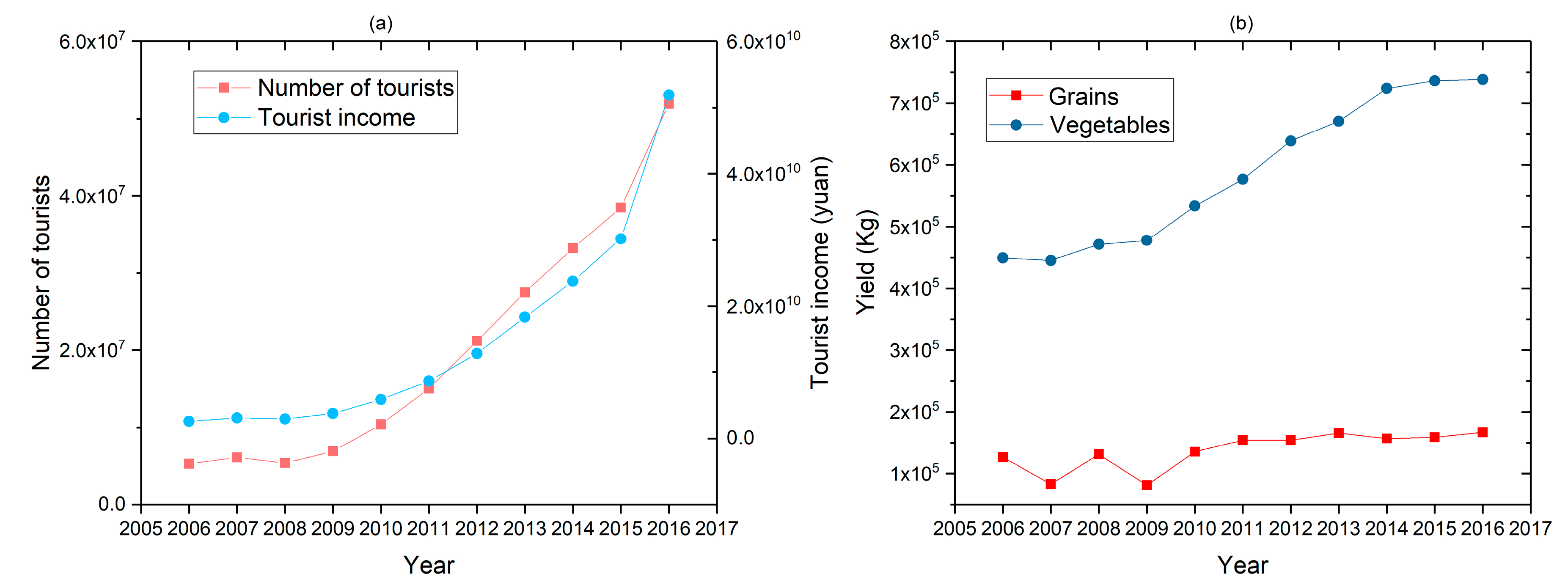
By sorting out the bulletin data, we found that there was a significant increase in tourism income and crop yields (Figure 9). After 2009, the tourism in the BS region rapidly developed (Figure 9a). In 2016, the number of tourists and tourism income were respectively increased by 10 times and 20 times compared with those in 2006. The percentage of urban water use (including residential water, urban public water and ecological water supply) increased from 22.8% in 2010 to 38.5% in 2015, whereas industrial and resident populations were stable.
Except 2007 and 2009, the grain yield in other years was stable, but the vegetable yield continued to grow in the period between 2009 and 2014 (Figure 9b). Although there was less precipitation in 2007 and 2009, vegetable yields did not significantly reduce compared to grain yields. The increase in vegetable yield directly lead to an increase in irrigation water consumption. According to the Water Resources Bulletin, groundwater supply accounts for more than 80% of the total water supply and irrigation water is the largest proportion of water consumption.
In the water resources bulletin of Hebei Province, the amount of irrigation water in ZJK was obtained from the boundary of the administrative district. Integrating the results of the human-induced factor evaluation index , ZJK’s irrigation information was obtained. Analysis of the bulletin data and , the correlation coefficient is 0.52. This indicates that can reflect the influence of human factors on irrigation water to a certain extent.
4. Discussion
4.1. Does the Change in Tourism Patterns Increase Groundwater Consumption?
In this study, the groundwater level changes are shown in Figure 3b. After 2014, the downward trend of groundwater level became more significant. Although vegetation affected by human-induced factors increased groundwater consumption, the declining period of groundwater level was beyond the growth period of vegetation. From the beginning of 2014 to the end of 2016, the declining duration of groundwater level became longer (from July to February of the next year). Before 2014, the declining duration of groundwater level in most years was from July to November. In this section, the impact of tourism on groundwater was discussed below.
Tourism is highly dependent on freshwater resources and become an important factor of fresh water resources in some tourism cities. Fresh water resources are consumed in different ways and the direct ways for tourists to use water include washing and using toilets. Simultaneously, the provider of tourism resources will provide tourists with corresponding tourism services including ski and golf (snowmaking and irrigation). In addition, fresh water resources are also used to maintain the gardens and landscapes of hotels and attractions [75,76,77]. In recent years, the tourism in the BS region has changed from traditional tourism mode to diversified tourism mode and more and more entertainment facilities (golf and ski) have been built in this region. Especially in 2015, the project of the 2022 Winter Olympics in ZJK greatly stimulated the development of skiing activities. The number of tourists in 2016 increased more significantly than that in other years (Figure 8a). However, the data were refreshed again in 2017. According to statistics data, the number of tourists in this region reached 62.598 million in 2017. Snowmaking consume lots of water and snowmaking in the USA in May 2004 consumed approximately 60 million m3 of water [78]. Alpine winter sports require a snow depth of ≥30 cm [79], but natural snowfall in the study area does not meet the standard (the average annual snowfall is less than 20 mm). Based on ski pistes length, energy consumption and information, Rixen et al. [80] estimated the water consumption in snowmaking and calculated the water consumption required for different lengths of ski pistes, 3 million m3 for 125 km long ski pistes consumed and 2 million m3 for 80 km long ski pistes. According to the length of ski pistes and other environmental conditions, the water consumption in snowmaking in BS is higher. As people become more enthusiastic about skiing, more and more people will participate in skiing. Therefore, the water resource management department should reasonably assess the water consumption in skiing.
GWSC in the BS region in different seasons was calculated (Table 1) and the CSR and JPL data were averaged to reduce the difference between different data resources. Dividing GWSC into recharge results and discharge results in different seasons can help us better understand the influences of human-induced factors on groundwater. In Q1th, GWSC increased significantly after 2011. Based on the results discussed in this section, we believed that snow (snow-making and snowfall) melt to supplement groundwater. In Q2nd and Q3rd, the recharge in GWSC was ascribed to precipitation and irrigation infiltration and the discharge was mainly from irrigation. After 2011, the discharge in groundwater in Q2nd was more significant than that in Q2nd in previous years. Although the groundwater discharge in Q3rd did not change significantly, the recharge in groundwater was reduced under the conditions of increased precipitation. The increase in vegetable yields is indicative of an increase in planting area, vegetation increased the absorption of precipitation by the soil layer and reduced infiltration. In Q4th, the groundwater recharge was zero after 2011 and groundwater discharge was the most significant in 2015. Skiing brings tourism resources while increasing the consumption of water. The non-agricultural water utilization in Q1th and Q4th also plays an important role in groundwater consumption (Table 1).
4.2. Comparison of Human-Induced Factor Assessment Methods Proposed in This Study with Other Methods.
The RUE method proposed in the study was compared with other RUE calculation methods and the RUE index was calculated in order to assess the influences of human-induced factors on vegetation [46,49,52,81,82,83]. Zhang et al. [53] improved the RUE model and assessed human-induced factors in arid regions with the improved model. Taking Region A and Region C as examples, the annual was not significantly correlated with GWSA. Therefore, the method cannot assess human activities in the BS region (Figure 10, Table 2 and Table 3).
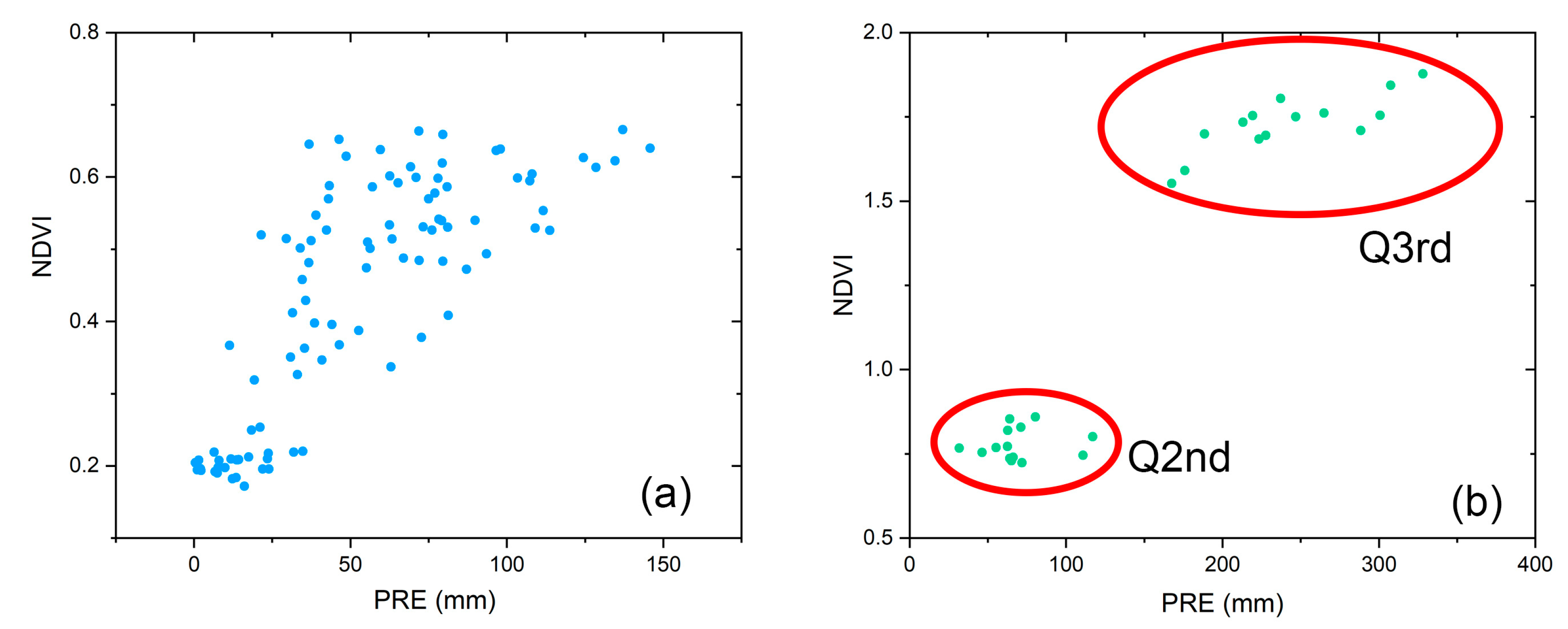
Propastin et al. [84] also proposed a method for assessing human-induced factors based on the linear relationship between NDVI and precipitation in arid regions. However, human activities in the BS region are frequent and linear regression cannot achieve the expected results (Figure 11a). Wang et al. [48] found that average NDVI values in the growing season were highly correlated with precipitation received during the growing season. Based on the correlation, we converted monthly-scale data into seasonal scale. After the conversion, we could analyze the influences of human-induced factors on vegetation more clearly. The advantage of and liner relationship methods were that they could reasonably assess the influences of human-induced factors in arid regions, but these methods led to the deviations in agricultural areas with more precipitation and more human activities.
The study area has the same NDVI value but different precipitation in Q2nd or Q3rd (Figure 11b). The method proposed in this paper can be used to evaluate the influences of human-induced factors on vegetation by calculating the relative membership of each pixel (NDVI and precipitation) in time series. The advantage of this method is that it can be used in agricultural areas and unstable precipitation areas because both linear correlation method and the methods based on the assumption of stable human activities were limited in the study area where the liner correlation between NDVI and precipitation was not significant. Taking Q3rd as an example, according to the method proposed in the study, it is assumed that the pixels with the maximum precipitation rarely require human activities, whereas the pixels with the least precipitation require more human activities to maintain vegetation growth. For time series pixels, if the precipitation is the same, but the NDVI is different, indicating that human-induced factors affect vegetation growth. If NDVI is the same, but the precipitation is different, it indicates that the pixel with less precipitation is more likely to be affected by human-induced factors. Two cases should be considered in the calculation of . In the first case, when the equals 0, the calculation result of will overflow. In the second case, when the equals 1, the calculation result of will be no less than 1. To prevent arithmetic overflow and misclassification, we make decisions on the calculation pixels (Equation (10)):
where dry land and irrigation are land types of pixels.
In this study, the judgment of the pixel land type should consider the two cases of maximum precipitation and minimum precipitation. In the rainfed land time series, when the precipitation reaches its maximum value, the NDVI also reaches the maximum value, and vice versa. Irrigation land is irrigated with additional water and vegetation growth varies slightly with precipitation. If necessary, standard deviations can also be introduced to assess the stability degree of precipitation and NDVI for decision making. Compensation can be used to remove some bad points of the results calculated by , but some bad points are still not compensated, such as NDVI influenced by cloud. Although the method proposed in this study cannot consider all cases, it can basically meet the application requirements.
5. Conclusions
In order to explore the causes for the decline of groundwater level in the BS region, we explore multiple factors such as crop pattern change and tourism. After comparing various methods for assessing the influence of human factors on vegetation, we decided to improve the RUE calculation method and obtained . Finally, the area affected by human-induced factors in different growth seasons of vegetation in the BS region was estimated. The increased area affected by human-induced factors accelerated groundwater consumption. Bulletin data indicated that the area planted with vegetables increased rapidly. As vegetables consumed more water resources than grains, groundwater consumption in Q2 and Q3rd was accelerated.
We also found that the groundwater level in the BS region still declined in Q4th (after 2014). Due to the rapid development of skiing in the BS region, more and more ski pistes were established in this region. Many studies showed that snowmaking required a large quantity of fresh water. We thought that the main cause for the decline of groundwater level in the BS region Q4th was snowmaking. Moreover, compared with previous methods, the method proposed in this paper could more effectively evaluate the influences of human factors on vegetation in the BS region, and result had a significant negative correlation with the decline of groundwater. Therefore, the water resource management department of the BS region not only needs to manage crop pattern, but also pays attention to the changes in social water use.
In the study, we explored the causes for groundwater level decline in the BS region and improved the RUE calculation method for assessing the influences of human-induced factors on vegetation. Through combining multi-source data, we explored the internal relationships of the data with different spatial and temporal resolutions. The study provides the guidance for evaluating the influences of human-induced factors on vegetation in the region with unstable precipitation and frequent human activities. The GRACE-FO satellite will be launched soon, it will provide more data for groundwater monitoring. In future research, we want to introduce more data of different sources and use multi-source data combination methods to improve the evaluation accuracy of the influences of human-induced factors on the environment.
Author Contributions
H.Z., H.Z., Z.H. designed the experiment; C.Z. and H.Z. provided revisions to the paper; H.W. and H.Z. provided the financial support; Z.H. wrote the manuscript.
Funding
National Key R&D Program of China (Grant No. 2018YFC0407705), the Fundamental Research Funds for the China Institute of Water Resources and Hydropower Research (WR0145B012017), and the Special Fund for Transformation of Scientific and Technological Achievements of China Institute of Water Resources and Hydropower Research (WR1003A112016).
Acknowledgments
We would like to acknowledgement Wei Feng for his help in GRACE data processing. GRACE Tellus land grids are available at http://grace.jpl.nasa.gov, supported by the NASA Measures Program. The CSR GRACE RL05 mascons solutions were downloaded from http://www.csr.utexas.edu/grace. MOD13A3 were downloaded from https://search.earthdata.nasa.gov/. Monthly precipitation gridded products are available at http://data.cma.cn/. ZJK and BS statistical bulletins on national economic and social development were obtained from http://www.zjktj.gov.cn/ and BS http://tjj.xlgl.gov.cn/, respectively.
Conflicts of Interest
The authors declare no conflict of interest.
References
- Aeschbach-Hertig, W.; Gleeson, T. Regional strategies for the accelerating global problem of groundwater depletion. Nat. Geosci. 2012, 5, 853–861. [Google Scholar] [CrossRef]
- Taylor, R.G.; Scanlon, B.; Döll, P.; Rodell, M.; Van Beek, R.; Wada, Y.; Longuevergne, L.; Leblanc, M.; Famiglietti, J.S.; Edmunds, M.; et al. Ground water and climate change. Nat. Clim. Chang. 2013, 3, 322–329. [Google Scholar] [CrossRef]
- Rodell, M.; Velicogna, I.; Famiglietti, J.S. Satellite-based estimates of groundwater depletion in India. Nature 2009, 460, 999–1002. [Google Scholar] [CrossRef] [PubMed] [Green Version]
- Guo, Z.; Huang, N.; Dong, Z.; Van Pelt, R.S.; Zobeck, T.M. Wind erosion induced soil degradation in Northern China: Status, measures and perspective. Sustainability 2014, 6, 8951–8966. [Google Scholar] [CrossRef]
- Song, C.; Yan, J.; Sha, J.; He, G.; Lin, X.; Ma, Y. Dynamic modeling application for simulating optimal policies on water conservation in Zhangjiakou City, China. J. Clean. Prod. 2018, 201, 111–122. [Google Scholar] [CrossRef]
- Piao, S.; Ciais, P.; Huang, Y.; Shen, Z.; Peng, S.; Li, J.; Zhou, L.; Liu, H.; Ma, Y.; Ding, Y.; et al. The impacts of climate change on water resources and agriculture in China. Nature 2010, 467, 43–51. [Google Scholar] [CrossRef] [PubMed]
- Shi, Y.; Shen, Y.; Kang, E.; Li, D.; Ding, Y.; Zhang, G.; Hu, R. Recent and future climate change in northwest China. Clim. Chang. 2007, 80, 379–393. [Google Scholar] [CrossRef]
- Alley, W.M.; Healy, R.W.; LaBaugh, J.W.; Reilly, T.E. Flow and storage in groundwater systems. Science 80- 2002, 296, 1985–1990. [Google Scholar] [CrossRef] [PubMed]
- Yang, Y.; Yang, Y.; Moiwo, J.P.; Hu, Y. Estimation of irrigation requirement for sustainable water resources reallocation in North China. Agric. Water Manag. 2010, 97, 1711–1721. [Google Scholar] [CrossRef]
- Wada, Y.; Van Beek, L.P.H.; Van Kempen, C.M.; Reckman, J.W.T.M.; Vasak, S.; Bierkens, M.F.P. Global depletion of groundwater resources. Geophys. Res. Lett. 2010, 37. [Google Scholar] [CrossRef] [Green Version]
- Feng, W.; Zhong, M.; Lemoine, J.M.; Biancale, R.; Hsu, H.T.; Xia, J. Evaluation of groundwater depletion in North China using the Gravity Recovery and Climate Experiment (GRACE) data and ground-based measurements. Water Resour. Res. 2013, 49, 2110–2118. [Google Scholar] [CrossRef] [Green Version]
- Döll, P. Vulnerability to the impact of climate change on renewable groundwater resources: A global-scale assessment. Environ. Res. Lett. 2009, 4. [Google Scholar] [CrossRef]
- Green, T.R.; Taniguchi, M.; Kooi, H.; Gurdak, J.J.; Allen, D.M.; Hiscock, K.M.; Treidel, H.; Aureli, A. Beneath the surface of global change: Impacts of climate change on groundwater. J. Hydrol. 2011, 405, 532–560. [Google Scholar] [CrossRef]
- Feng, W.; Shum, C.K.; Zhong, M.; Pan, Y. Groundwater storage changes in China from satellite gravity: An overview. Remote Sens. 2018, 10, 674. [Google Scholar] [CrossRef]
- Scanlon, B.R.; Jolly, I.; Sophocleous, M.; Zhang, L. Global impacts of conversions from natural to agricultural ecosystems on water resources: Quantity versus quality. Water Resour. Res. 2007, 43. [Google Scholar] [CrossRef] [Green Version]
- Xie, Y.; Huang, S.; Liu, S.; Leng, G.; Peng, J.; Huang, Q.; Li, P. GRACE-based terrestrialwater storage in Northwest China: Changes and causes. Remote Sens. 2018, 10, 1163. [Google Scholar] [CrossRef]
- Yeh, P.J.F.; Swenson, S.C.; Famiglietti, J.S.; Rodell, M. Remote sensing of groundwater storage changes in Illinois using the Gravity Recovery and Climate Experiment (GRACE). Water Resour. Res. 2006, 42, 1–7. [Google Scholar] [CrossRef]
- Yang, P.; Chen, Y. An analysis of terrestrial water storage variations from GRACE and GLDAS: The Tianshan Mountains and its adjacent areas, central Asia. Quat. Int. 2015, 358, 106–112. [Google Scholar] [CrossRef]
- Seyoum, W.M.; Milewski, A.M. Monitoring and comparison of terrestrial water storage changes in the northern high plains using GRACE and in-situ based integrated hydrologic model estimates. Adv. Water Resour. 2016, 94, 31–44. [Google Scholar] [CrossRef]
- Forootan, E.; Rietbroek, R.; Kusche, J.; Sharifi, M.A.; Awange, J.L.; Schmidt, M.; Omondi, P.; Famiglietti, J. Separation of large scale water storage patterns over Iran using GRACE, altimetry and hydrological data. Remote Sens. Environ. 2014, 140, 580–595. [Google Scholar] [CrossRef] [Green Version]
- Lenk, O. Satellite based estimates of terrestrial water storage variations in Turkey. J. Geodyn. 2013, 67, 106–110. [Google Scholar] [CrossRef]
- Frappart, F.; Ramillien, G. Monitoring groundwater storage changes using the Gravity Recovery and Climate Experiment (GRACE) satellite mission: A review. Remote Sens. 2018, 10, 829. [Google Scholar] [CrossRef]
- Zhong, Y.; Zhong, M.; Feng, W.; Wu, D. Groundwater Depletion in the West Liaohe River Basin, China and Its Implications Revealed by GRACE and In Situ Measurements. Remote Sens. 2018, 10, 493. [Google Scholar] [CrossRef]
- Chen, X.; Jiang, J.; Li, H. Drought and flood monitoring of the Liao River Basin in Northeast China using extended GRACE data. Remote Sens. 2018, 10, 1168. [Google Scholar] [CrossRef]
- Döll, P.; Müller Schmied, H.; Schuh, C.; Portmann, F.T.; Eicker, A. Global-scale assessment of groundwater depletion and related groundwater abstractions: Combining hydrological modeling with information from well observations and GRACE satellites. Water Resour. Res. 2014, 50, 5698–5720. [Google Scholar] [CrossRef] [Green Version]
- Marc, F.P. Bierkens Global hydrology 2015: State, trends, and directions. Water Resour. Res. 2016, 51, 600–612. [Google Scholar] [CrossRef]
- Rodell, M.; Houser, P.R.; Jambor, U.; Gottschalck, J.; Mitchell, K.; Meng, C.J.; Arsenault, K.; Cosgrove, B.; Radakovich, J.; Bosilovich, M.; et al. The Global Land Data Assimilation System. Bull. Am. Meteorol. Soc. 2004, 85, 381–394. [Google Scholar] [CrossRef] [Green Version]
- Tapley, B.D.; Bettadpur, S.; Ries, J.C.; Thompson, P.F.; Watkins, M.M. GRACE measurements of mass variability in the Earth system. Science 80- 2004, 305, 503–505. [Google Scholar] [CrossRef] [PubMed]
- Chen, J.L.; Rodell, M.; Wilson, C.R.; Famiglietti, J.S. Low degree spherical harmonic influences on Gravity Recovery and Climate Experiment (GRACE) water storage estimates. Geophys. Res. Lett. 2005, 32. [Google Scholar] [CrossRef] [Green Version]
- Tiwari, V.M.; Wahr, J.; Swenson, S. Dwindling groundwater resources in northern India, from satellite gravity observations. Geophys. Res. Lett. 2009, 36. [Google Scholar] [CrossRef] [Green Version]
- Long, D.; Chen, X.; Scanlon, B.R.; Wada, Y.; Hong, Y.; Singh, V.P.; Chen, Y.; Wang, C.; Han, Z.; Yang, W. Have GRACE satellites overestimated groundwater depletion in the Northwest India Aquifer? Sci. Rep. 2016, 6. [Google Scholar] [CrossRef] [PubMed]
- Famiglietti, J.S.; Lo, M.; Ho, S.L.; Bethune, J.; Anderson, K.J.; Syed, T.H.; Swenson, S.C.; De Linage, C.R.; Rodell, M. Satellites measure recent rates of groundwater depletion in California’s Central Valley. Geophys. Res. Lett. 2011, 38, 2–5. [Google Scholar] [CrossRef]
- Scanlon, B.R.; Longuevergne, L.; Long, D. Ground referencing GRACE satellite estimates of groundwater storage changes in the California Central Valley, USA. Water Resour. Res. 2012, 48. [Google Scholar] [CrossRef] [Green Version]
- Huang, Z.; Pan, Y.; Gong, H.; Yeh, P.J.F.; Li, X.; Zhou, D.; Zhao, W. Subregional-scale groundwater depletion detected by GRACE for both shallow and deep aquifers in North China Plain. Geophys. Res. Lett. 2015, 42, 1791–1799. [Google Scholar] [CrossRef] [Green Version]
- Nanteza, J.; de Linage, C.R.; Thomas, B.F.; Famiglietti, J.S. Monitoring groundwater storage changes in complex basement aquifers: An evaluation of the GRACE satellites over East Africa. Water Resour. Res. 2016, 52, 9542–9564. [Google Scholar] [CrossRef] [Green Version]
- Bonsor, H.C.; Shamsudduha, M.; Marchant, B.P.; MacDonald, A.M.; Taylor, R.G. Seasonal and decadal groundwater changes in African sedimentary aquifers estimated using GRACE products and LSMs. Remote Sens. 2018, 10, 904. [Google Scholar] [CrossRef]
- Zhao, W.Z.; Xiao, H.L.; Liu, Z.M.; Li, J. Soil degradation and restoration as affected by land use change in the semiarid Bashang area, northern China. Catena 2005, 59, 173–186. [Google Scholar] [CrossRef]
- Tian, X.; Chen, M.; Liu, L. Study on the changes of hydrogeological conditions in Bashang area of Zhangjiakou City. Geol. Hebei 2015, 32–34. [Google Scholar]
- Scanlon, B.R.; Zhang, Z.; Save, H.; Sun, A.Y.; Müller Schmied, H.; van Beek, L.P.H.; Wiese, D.N.; Wada, Y.; Long, D.; Reedy, R.C.; et al. Global models underestimate large decadal declining and rising water storage trends relative to GRACE satellite data. Proc. Natl. Acad. Sci. USA 2018, 201704665. [Google Scholar] [CrossRef] [PubMed]
- Liang, X.; Lettenmaier, D.P.; Wood, E.F.; Burges, S.J. A simple hydrologically based model of land surface water and energy fluxes for general circulation models. J. Geophys. Res. 1994, 99, 14415. [Google Scholar] [CrossRef]
- Koster, R.D.; Suarez, M.J. Modeling the Land Surface Boundar in Climate Models as a Composite of independent Vegetation Stands. J. Geophys. Res. 1992, 97, 2697–2715. [Google Scholar] [CrossRef]
- Ek, M.B. Implementation of Noah land surface model advances in the National Centers for Environmental Prediction operational mesoscale Eta model. J. Geophys. Res. 2003, 108, 8851. [Google Scholar] [CrossRef]
- Dai, Y.; Zeng, X.; Dickinson, R.E.; Baker, I.; Bonan, G.B.; Bosilovich, M.G.; Denning, A.S.; Dirmeyer, P.A.; Houser, P.R.; Niu, G.; et al. The Common Land Model (CLM). Bull. Am. Meteorol. Soc. 2001, 1013–1023. [Google Scholar] [CrossRef]
- Strassberg, G.; Scanlon, B.R.; Rodell, M. Comparison of seasonal terrestrial water storage variations from GRACE with groundwater-level measurements from the High Plains Aquifer (USA). Geophys. Res. Lett. 2007, 34. [Google Scholar] [CrossRef] [Green Version]
- Diouf, A.; Lambin, E.F. Monitoring land-cover changes in semi-arid regions: Remote sensing data and field observations in the Ferlo, Senegal. J. Arid Environ. 2001, 48, 129–148. [Google Scholar] [CrossRef]
- Huxman, T.E.; Smith, M.D.; Fay, P.A.; Knapp, A.K.; Shaw, M.R.; Loik, M.E.; Smith, S.D.; Tissue, D.T.; Zak, J.C.; Weltzin, J.F.; et al. Convergence across biomes to common rain use efficiency. Nature 2004, 429, 651–654. [Google Scholar] [CrossRef] [PubMed]
- Wessels, K.J.; Prince, S.D.; Malherbe, J.; Small, J.; Frost, P.E.; VanZyl, D. Can human-induced land degradation be distinguished from the effects of rainfall variability? A case study in South Africa. J. Arid Environ. 2007, 68, 271–297. [Google Scholar] [CrossRef]
- Wang, J.; Rich, P.M.; Price, K.P. Temporal responses of NDVI to precipitation and temperature in the central Great Plains, USA. Int. J. Remote Sens. 2003, 24, 2345–2364. [Google Scholar] [CrossRef] [Green Version]
- Holm, A.M.R.; Cridland, S.W.; Roderick, M.L. The use of time-integrated NOAA NDVI data and rainfall to assess landscape degradation in the arid shrubland of Western Australia. Remote Sens. Environ. 2003, 85, 145–158. [Google Scholar] [CrossRef]
- Bai, Z.; Dent, D. Recent land degradation and improvement in China. Ambio 2009, 38, 150–156. [Google Scholar] [CrossRef] [PubMed]
- Veron, S.R.; Oesterheld, M.; Paruelo, J.M. Production as a function of resource availability: slope and efficiences are different. J. Veg. Sci. 2005, 16, 351–354. [Google Scholar] [CrossRef]
- Fensholt, R.; Rasmussen, K. Analysis of trends in the Sahelian “rain-use efficiency” using GIMMS NDVI, RFE and GPCP rainfall data. Remote Sens. Environ. 2011, 115, 438–451. [Google Scholar] [CrossRef]
- Zhang, X.; Wang, N.; Xie, Z.; Ma, X.; Huete, A. Water loss due to increasing planted vegetation over the Badain Jaran Desert, China. Remote Sens. 2018, 10, 134. [Google Scholar] [CrossRef]
- Shouyu, C.; Guangtao, F. A DRASTIC-based fuzzy pattern recognition methodology for groundwater vulnerability evaluation. Hydrol. Sci. J. 2003, 48, 211–220. [Google Scholar] [CrossRef]
- Weijie, H.; Hailong, L.; Anming, B.; El-Tantawi, A.M. Influences of environmental changes on water storage variations in Central Asia. J. Geogr. Sci. 2018, 28, 985–1000. [Google Scholar] [CrossRef]
- Fensholt, R.; Proud, S.R. Evaluation of Earth Observation based global long term vegetation trends—Comparing GIMMS and MODIS global NDVI time series. Remote Sens. Environ. 2012, 119, 131–147. [Google Scholar] [CrossRef]
- Wardlow, B.D.; Egbert, S.L. Large-area crop mapping using time-series MODIS 250 m NDVI data: An assessment for the U.S. Central Great Plains. Remote Sens. Environ. 2008, 112, 1096–1116. [Google Scholar] [CrossRef]
- Lunetta, R.S.; Knight, J.F.; Ediriwickrema, J.; Lyon, J.G.; Worthy, L.D. Land-cover change detection using multi-temporal MODIS NDVI data. Remote Sens. Environ. 2006, 105, 142–154. [Google Scholar] [CrossRef]
- Anyamba, A.; Tucker, C.J. Analysis of Sahelian vegetation dynamics using NOAA-AVHRR NDVI data from 1981–2003. J. Arid Environ. 2005, 63, 596–614. [Google Scholar] [CrossRef]
- Carlson, T.C.; Ripley, D.A. On the relationship between NDVI, fractional vegetation cover, and leaf area index. Remote Sens. Environ. 1997, 62, 241–252. [Google Scholar] [CrossRef]
- Cheng, M.; Tapley, B.D. Variations in the Earth’s oblateness during the past 28 years. J. Geophys. Res. Solid Earth 2004, 109. [Google Scholar] [CrossRef]
- Swenson, S.; Chambers, D.; Wahr, J. Estimating geocenter variations from a combination of GRACE and ocean model output. J. Geophys. Res. Solid Earth 2008, 113. [Google Scholar] [CrossRef] [Green Version]
- Jacob, T.; Wahr, J.; Pfeffer, W.T.; Swenson, S. Recent contributions of glaciers and ice caps to sea level rise. Nature 2012, 482, 514–518. [Google Scholar] [CrossRef] [PubMed]
- Swenson, S.; Wahr, J. Post-processing removal of correlated errors in GRACE data. Geophys. Res. Lett. 2006, 33. [Google Scholar] [CrossRef] [Green Version]
- Melzer, B.A.; Subrahmanyam, B. Evaluation of GRACE Mascon Gravity Solution in Relation to Interannual Oceanic Water Mass Variations. IEEE Trans. Geosci. Remote Sens. 2017, 55, 907–914. [Google Scholar] [CrossRef]
- Save, H.; Bettadpur, S.; Tapley, B.D. High-resolution CSR GRACE RL05 mascons. J. Geophys. Res. Solid Earth 2016, 121, 7547–7569. [Google Scholar] [CrossRef]
- Wiese, D.N.; Landerer, F.W.; Watkins, M.M. Quantifying and reducing leakage errors in the JPL RL05M GRACE mascon solution. Water Resour. Res. 2016, 52, 7490–7502. [Google Scholar] [CrossRef]
- Shamsudduha, M.; Taylor, R.G.; Longuevergne, L. Monitoring groundwater storage changes in the highly seasonal humid tropics: Validation of GRACE measurements in the Bengal Basin. Water Resour. Res. 2012, 48. [Google Scholar] [CrossRef] [Green Version]
- Syed, T.H.; Famiglietti, J.S.; Rodell, M.; Chen, J.; Wilson, C.R. Analysis of terrestrial water storage changes from GRACE and GLDAS. Water Resour. Res. 2008, 44. [Google Scholar] [CrossRef] [Green Version]
- Zaitchik, B.F.; Rodell, M.; Olivera, F. Evaluation of the Global Land Data Assimilation System using global river discharge data and a source-to-sink routing scheme. Water Resour. Res. 2010, 46. [Google Scholar] [CrossRef] [Green Version]
- China Institute of Geological Environment Monitoring, (CIGEM). China Geological Environment Monitoring: Groundwater Yearbook; China Land Press: Beijing, China, 2007; pp. 62–82. ISBN 9787802461499. [Google Scholar]
- Water Resources Department of Hebei Province. Hebei Provincial Water Resources Bulletin, 2003–2016; Water Resources Department of Hebei Province: Shijiazhuang, China, 2012; pp. 11–13.
- Landerer, F.W.; Swenson, S.C. Accuracy of scaled GRACE terrestrial water storage estimates. Water Resour. Res. 2012, 48. [Google Scholar] [CrossRef] [Green Version]
- Bridget, R.S.; Zhang, Z.; Save, H.; Wiese, D.N.; Landerer, F.W.; Long, D.; Laurent, L.; Chen, J. Global evaluation of new GRACEmascon products for hydrologic applications. Water Resour. Res. 2016, 9412–9429. [Google Scholar] [CrossRef]
- Gössling, S. The consequences of tourism for sustainable water use on a tropical island: Zanzibar, Tanzania. J. Environ. Manag. 2001, 61, 179–191. [Google Scholar] [CrossRef] [PubMed]
- Chapagain, A.K.; Hoekstra, A.Y. The global component of freshwater demand and supply: An assessment of virtual water flows between nations as a result of trade in agricultural and industrial products. Water Int. 2008, 33, 19–32. [Google Scholar] [CrossRef]
- Gössling, S.; Peeters, P.; Hall, C.M.; Ceron, J.P.; Dubois, G.; Lehmann, L.V.; Scott, D. Tourism and water use: Supply, demand, and security. An international review. Tour. Manag. 2012, 33. [Google Scholar] [CrossRef]
- Scott, D.; Hall, C.; Stefan, G. Tourism and Climate Change; Routledge: London, UK, 2012; pp. 1–14. [Google Scholar]
- Elsasser, H.; Messerli, P. The Vulnerability of the Snow Industry in the Swiss Alps. Mt. Res. Dev. 2001, 21, 335–339. [Google Scholar] [CrossRef]
- Rixen, C.; Teich, M.; Lardelli, C.; Gallati, D.; Pohl, M.; Pütz, M.; Bebi, P. Winter Tourism and Climate Change in the Alps: An Assessment of Resource Consumption, Snow Reliability, and Future Snowmaking Potential. Mt. Res. Dev. 2011, 31, 229–236. [Google Scholar] [CrossRef]
- Sileshi, G.W.; Akinnifesi, F.K.; Ajayi, O.C.; Muys, B. Integration of legume trees in maize-based cropping systems improves rain use efficiency and yield stability under rain-fed agriculture. Agric. Water Manag. 2011, 98, 1364–1372. [Google Scholar] [CrossRef]
- Yang, Y.; Fang, J.; Fay, P.A.; Bell, J.E.; Ji, C. Rain use efficiency across a precipitation gradient on the Tibetan Plateau. Geophys. Res. Lett. 2010, 37. [Google Scholar] [CrossRef] [Green Version]
- Fensholt, R.; Rasmussen, K.; Kaspersen, P.; Huber, S.; Horion, S.; Swinnen, E. Assessing land degradation/recovery in the african sahel from long-term earth observation based primary productivity and precipitation relationships. Remote Sens. 2013, 5, 664–686. [Google Scholar] [CrossRef]
- Propastin, P.A.; Kappas, M.; Muratova, N.R. A remote sensing based monitoring system for discrimination between climate and human-induced vegetation change in Central Asia. Manag. Environ. Qual. An Int. J. 2008, 19, 579–596. [Google Scholar] [CrossRef]
Figure 1.
Spatial location and elevation map of the study area.

Figure 2.
Study flowchart of the groundwater decline in the BS region. GRACE: Gravity Recovery and Climate Experiment. RUE: rain use efficiency.
Figure 2.
Study flowchart of the groundwater decline in the BS region. GRACE: Gravity Recovery and Climate Experiment. RUE: rain use efficiency.

Figure 3.
Time series of water storage changes from 2003 to 2016. (a) shows the monthly TWSA (derived from CSR and JPL) and yearly PRE from 2003 to 2016; (b) shows the time series of GWSA derived from GRACE and GLDAS. GWLA: groundwater level anomalies; JPL: Jet Propulsion Laboratory; PRE: precipitation; CSR: Center for Space Research; EWH: Equivalent Water Height.

Figure 4.
Spatial distributions of terrestrial water storage anomalies (TWSA) and groundwater storage anomalies (GWSA) annual trends. (a) and (c) shows the trends of TWSA and GWSA based on CSR data, respectively. (b) and (d) shows the trends of TWSA and GWSA based on JPL data, respectively.
Figure 4.
Spatial distributions of terrestrial water storage anomalies (TWSA) and groundwater storage anomalies (GWSA) annual trends. (a) and (c) shows the trends of TWSA and GWSA based on CSR data, respectively. (b) and (d) shows the trends of TWSA and GWSA based on JPL data, respectively.

Figure 5.
Land cover and Normalized Difference Vegetation Index (NDVI) trends in the study area. (a) land cover in 2015 and (b) NDVI trends from 2003 to 2016.
Figure 5.
Land cover and Normalized Difference Vegetation Index (NDVI) trends in the study area. (a) land cover in 2015 and (b) NDVI trends from 2003 to 2016.

Figure 6.
Time series NDVI interval pixel statistics.

Figure 7.
time series calculation results of (a) Q2nd and (b) Q3rd. The greater the value is, the greater the influence of human-induced factors is.
Figure 7.
time series calculation results of (a) Q2nd and (b) Q3rd. The greater the value is, the greater the influence of human-induced factors is.


Figure 8.
(a) Changes (NDVI and precipitation) of time series of Q2nd and Q3rd in different regions (Region A is Xilin Gol; Region B and Region C are eastern and central-western part of the study area, respectively). The green and blue dashed lines represent the liner trends of NDVI and precipitation, respectively. (b) Changes ( and GWSA) of time series of Q2nd and Q3rd in different regions. The tables in the figure show the correlation coefficient between and GWSA (CSR and JPL).

Figure 9.
Economic and social development statistical bulletin data from 2006 to 2016. (a) Number of tourists and tourist income; (b) yields of grains and vegetables.
Figure 9.
Economic and social development statistical bulletin data from 2006 to 2016. (a) Number of tourists and tourist income; (b) yields of grains and vegetables.

Figure 10.
Calculation results of .

Figure 11.
(a) Monthly correlation between NDVI and precipitation in vegetation growing season, (b) seasonal correlation between NDVI and precipitation in Q2nd and Q3rd.
Figure 11.
(a) Monthly correlation between NDVI and precipitation in vegetation growing season, (b) seasonal correlation between NDVI and precipitation in Q2nd and Q3rd.


Table 1.
Time series of GWSC seasonal division table.
| Q1th | Q2nd | Q3rd | Q4th | R-D | |||||
|---|---|---|---|---|---|---|---|---|---|
| R | D | R | D | R | D | R | D | ||
| 2003 | 0.00 | 2.10 | 1.68 | 0.00 | 2.05 | 1.02 | 0.28 | 3.15 | −2.26 |
| 2004 | 1.16 | 0.99 | 1.49 | 0.68 | 2.60 | 0.00 | 0.54 | 2.83 | 1.29 |
| 2005 | 2.87 | 2.77 | 2.05 | 0.12 | 0.52 | 0.56 | 0.79 | 1.49 | 1.29 |
| 2006 | 1.09 | 1.45 | 0.60 | 0.70 | 1.95 | 1.36 | 0.27 | 0.80 | −0.40 |
| 2007 | 0.90 | 1.09 | 0.64 | 0.00 | 0.36 | 0.76 | 0.33 | 1.86 | −1.48 |
| 2008 | 0.70 | 0.30 | 0.93 | 0.79 | 1.25 | 1.61 | 0.44 | 2.06 | −1.44 |
| 2009 | 1.45 | 0.00 | 0.68 | 0.31 | 1.02 | 1.11 | 3.81 | 3.15 | 2.39 |
| 2010 | 0.00 | 3.36 | 2.53 | 0.00 | 0.00 | 1.69 | 0.61 | 2.98 | −4.89 |
| 2011 | 0.00 | 1.00 | 4.28 | 0.00 | 1.41 | 1.24 | 0.06 | 1.67 | 1.84 |
| 2012 | 1.87 | 0.07 | 0.00 | 2.3. | 2.50 | 0.00 | 0.00 | 1.70 | 0.30 |
| 2013 | 2.04 | 0.39 | 0.36 | 0.92 | 0.90 | 1.14 | 1.51 | 0.00 | 2.36 |
| 2014 | 0.64 | 1.85 | 0.61 | 2.14 | 1.52 | 1.54 | 0.00 | 1.36 | −4.12 |
| 2015 | 3.48 | 2.83 | 2.53 | 2.98 | 1.85 | 1.85 | 0.00 | 5.26 | −5.06 |
| 2016 | 4.60 | 0.04 | 1.41 | 1.08 | 0.56 | 1.66 | 0.00 | 2.40 | 1.39 |
R represents recharge and D represents discharge. unit: mm.
Table 2.
Correlation between GWSA and in Region A.
| GWSA_CSR | GWSA_JPL | ||
|---|---|---|---|
| GWSA_CSR | 1 | ||
| GWSA_JPL | 0.98 | 1 | |
| 0.22 | 0.17 | 1 |
Table 3.
Correlation between GWSA and in Region C.
| GWSA_CSR | GWSA_JPL | ||
|---|---|---|---|
| GWSA_CSR | 1 | ||
| GWSA_JPL | 0.98 | 1 | |
| −0.34 | −0.36 | 1 |
© 2019 by the authors. Licensee MDPI, Basel, Switzerland. This article is an open access article distributed under the terms and conditions of the Creative Commons Attribution (CC BY) license (http://creativecommons.org/licenses/by/4.0/).
Share and Cite
MDPI and ACS Style
Hao, Z.; Zhao, H.; Zhang, C.; Zhou, H.; Zhao, H.; Wang, H. Correlation Analysis Between Groundwater Decline Trend and Human-Induced Factors in Bashang Region. Water 2019, 11, 473. https://doi.org/10.3390/w11030473
AMA Style
Hao Z, Zhao H, Zhang C, Zhou H, Zhao H, Wang H. Correlation Analysis Between Groundwater Decline Trend and Human-Induced Factors in Bashang Region. Water. 2019; 11(3):473. https://doi.org/10.3390/w11030473
Chicago/Turabian StyleHao, Zhen, Hesong Zhao, Chi Zhang, Huicheng Zhou, Hongli Zhao, and Hao Wang. 2019. "Correlation Analysis Between Groundwater Decline Trend and Human-Induced Factors in Bashang Region" Water 11, no. 3: 473. https://doi.org/10.3390/w11030473
Note that from the first issue of 2016, this journal uses article numbers instead of page numbers. See further details here.