Comparison of Conventional Deterministic and Entropy-Based Methods for Predicting Sediment Concentration in Debris Flow

Abstract

In this study, the distribution of sediment concentration and the mean sediment concentration in debris flow were investigated using deterministic and probabilistic approaches. Tsallis entropy and Shannon entropy have recently been employed to estimate these parameters. However, other entropy theories, such as the general index entropy and Renyi entropy theories, which are generalizations of the Shannon entropy, have not been used to derive the sediment concentration in debris flow. Furthermore, no comprehensive and rigorous analysis has been conducted to compare the goodness of fit of existing conventional deterministic methods and different entropy-based methods using experimental data collected from the literature. Therefore, this study derived the analytical expressions for the distribution of sediment concentration and the mean sediment concentration in debris flow based on the general index entropy and Renyi entropy theories together with the principle of maximum entropy and tested the validity of existing conventional deterministic methods as well as four different entropy-based expressions for the limited collected observational data. This study shows the potential of using the Tsallis entropy theory together with the principle of maximum entropy to predict sediment concentration in debris flow over an erodible channel bed.

1. Introduction

Debris flow is one of the disastrous geohazards in mountainous areas around the world. It is usually triggered by rainfall, earthquakes, and human activities and often has a destructive nature, thus greatly influencing human life and valuable property [1,2,3]. In recent decades, many debris flows have occurred, resulting in large losses. For example, on 7 August 2010, two large-scale debris flows occurred in both the Sanyanyu and Luojiayu valleys in the northern part of the city of Zhouqu, Northwest China, due to heavy rainfall in this area [4]. As a result, 1557 people living in this area were killed, and more than 5500 houses along the path of the debris flow were damaged. The two debris flows went across the deposition fans and flowed into the Bailong River. Consequently, a 550-m-long and 70-m-wide debris dam was formed, and one-third of the city was inundated for five days [5,6]. Debris flows in the southwest areas of Japan resulting from torrential rain in August 2014 led to more than 49 deaths and 47 missing people, while more than 1.6 million people were forced to flee from their hometowns [7]. Therefore, it is urgent to study debris flow to reduce its damage.

Debris flow is caused in three ways [8]: (1) the sediment particles from the gully beds are entrained by the water runoff; (2) a natural dam formed by a landslide fails; and (3) a landslide block is liquefied. This study focuses on the first cause. The properties of formation, movement, and deposition of debris flow and the prediction and mitigation of debris flow hazards are typical concerns of some investigations regarding debris flow [1,9,10,11]. However, beyond exploring these characteristics, the estimation of the sediment concentration in debris flow is also needed [12,13]. Some studies have shown that both debris flow and sediment-laden flow consist of very fine grains and that the only difference is the portion of fine grains in them [14,15,16,17]. Although a hydraulic model can be formulated for modeling debris flow, uncertainties in debris flow variables may limit its potential use [12,13]. A probability-based approach based on the entropy theory has been adopted by some authors for debris flow modeling. Lien and Tsai used the Shannon entropy to derive an expression for sediment concentration in debris flow [12], whereas Singh and Cui [13] employed the Tsallis entropy to model the sediment concentration in debris flow.

Other entropy theories, such as the general index entropy and Renyi entropy theories, which are generalizations of the Shannon entropy, have not been used for deriving the sediment concentration in debris flow. Furthermore, no comprehensive and rigorous analysis has been conducted to compare the goodness of fit of existing conventional deterministic methods and different entropy-based methods using the collected experimental data from the literature. Thus, this study attempted to explore the sediment concentration in debris flow based on the general index entropy and Renyi entropy theories and present a comparative analysis of the existing conventional deterministic methods with different entropy-based methods. The structure of this paper is as follows. Section 2 briefly introduces the existing conventional deterministic formulae for the distribution of sediment concentration in debris flow. Section 3 presents the derivations of the analytical expressions for the distribution of sediment concentration in debris flow based on the general index entropy and Renyi entropy theories as well as the developed Tsallis and Shannon entropy-based expressions. Section 4 tests the conventional deterministic formulae and different entropy-based expressions by comparing them with the collected experimental data from the literature. Finally, Section 5 presents the concluding remarks. The aim of this study was to model the variation in sediment concentration with the vertical distance from the channel bottom (i.e., distribution of sediment concentration) in debris flow and to determine the relationship between the mean sediment concentration in debris flow and the inclination of the channel bed from the horizontal line (their definitions will be elaborated on in the next section) using some conventional deterministic and entropy-based methods. This study shows the potential of using the Tsallis entropy theory together with the principle of maximum entropy to model the distribution of sediment concentration and the mean sediment concentration in debris flow. The Tsallis entropy theory can therefore be a good addition to some conventional deterministic models.

2. Conventional Deterministic Methods for Determining the Distribution of Sediment Concentration in Debris Flow

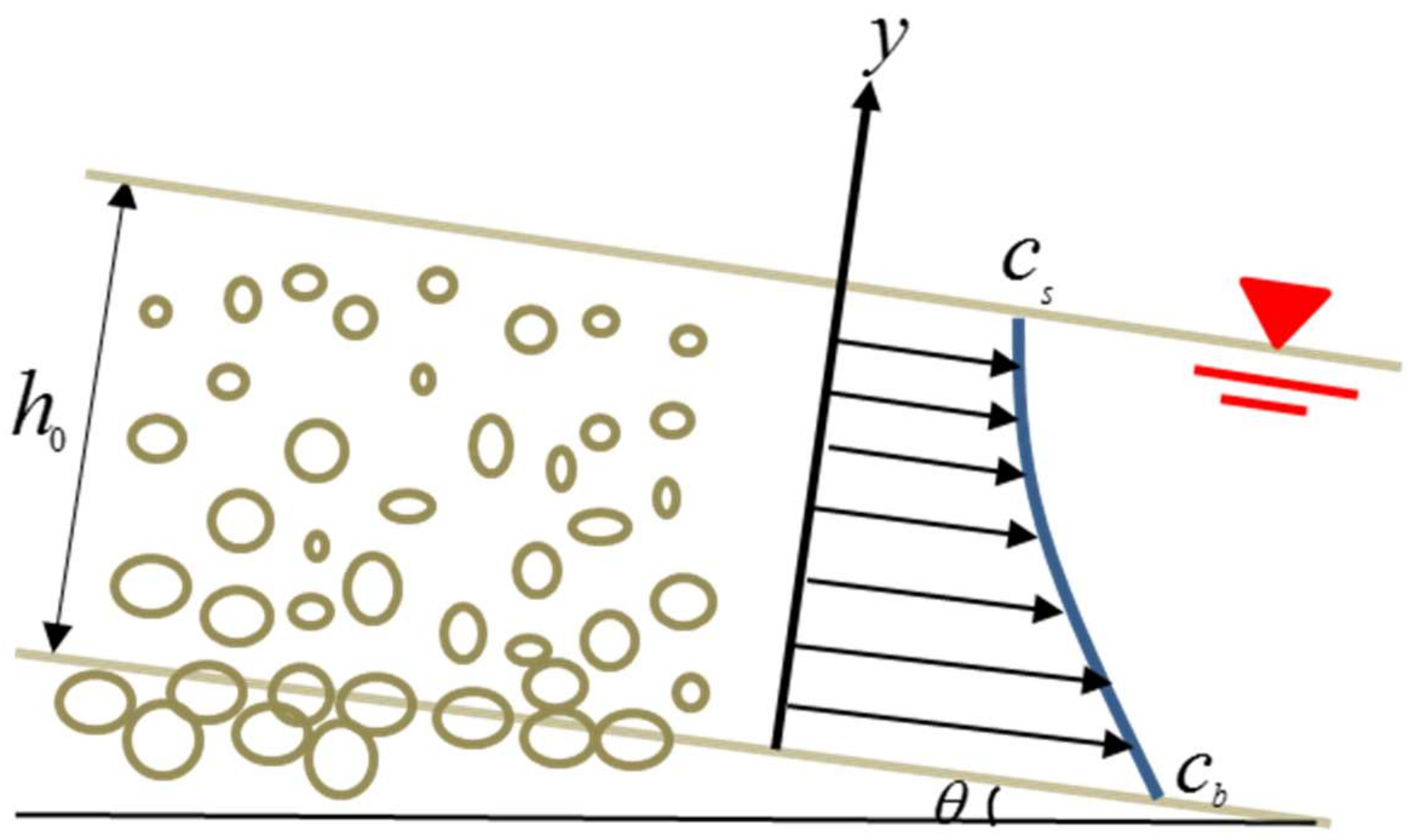
Figure 1 schematically shows debris flow over an erodible bed, as presented by Singh and Cui [13]. It is assumed that the debris flow is steady and uniform, which is reasonable according to Zhang [16] and Fei and Shu [17]. In this figure, $h_0$ is the flow depth, and the sediment concentration decreases monotonically from a maximum value of $c_b$ at the channel bottom to a value of $c_s$ at the flow surface. By defining $c\left(y\right)$ as the sediment concentration at a vertical distance $y$ from the channel bottom, $c_s\le c\left(y\right)\le c_b$. The sediment concentration is defined as the volume of sediment divided by the total volume of the fluid–sediment mixture and is thus nondimensional.

Based on the governing equations of the solid phase in debris flow movement, Tsubaki et al. [18] derived the following expression to estimate the vertical distribution of sediment concentration:

$$\frac{y}{h_0}=\left(2\frac{c_b-c}{c_b}-2\frac{c_a-c_s}{c_b}\ln \frac{c-c_a}{c_b-c_a}\right)\frac{\chi }{\psi }$$

(1)

where $\chi$ = 1/3, as suggested by Tsubaki et al. [18], and $c_a$ is the specific sediment concentration, which is estimated by the following expression:

$$c_a=\frac{\tan \theta }{\frac{\left({\rho }_s-\rho \right)}{\rho }\left({\alpha }_1-\tan \theta \right)}$$

(2)

The parameter $\psi$ is estimated as follows:

$$\psi =\frac{\left({\alpha }_1-\tan \theta \right)}{{\alpha }_1}$$

(3)

In Equations (2) and (3), $\theta$ is the inclination angle of the channel bed from the horizontal line, as also shown in Figure 1; ${\rho }_s$ is the density of sediment; and $\rho$ is the fluid density. The parameter ${\alpha }_1$ can be evaluated using the following formula by Tsubaki et al. [18]:

$${\alpha }_1=\frac{\left(0.0762+0.102\mu \right)/\left(0.0898-0.067\mu \right)}{1+\rho /\left(2\sigma \right)}$$

(4)

In Equation (4), $\mu$ = 0.1 was suggested by Tsubaki et al. [18].

Three kinds of conventional deterministic formulae can be used to estimate the mean sediment concentration in debris flow, $c_D$. Takahashi [8] theoretically derived a relationship to estimate the mean sediment concentration in debris flow occurring because of the mobilization of bed particles by water runoff. The relationship can be expressed as follows:

$$c_D=\frac{\rho \tan \theta }{\left({\rho }_s-\rho \right)\left(\tan \varphi -\tan \theta \right)}$$

(5)

where $\varphi$ is the angle of internal friction.

Based on the data sets of experimental flumes, Ou and Mizuyama [19] proposed an empirical relationship for the mean sediment concentration in debris flow by adopting the channel bed slope as the principal factor as follows:

$$c_D=\frac{4.3{\left(\tan \theta \right)}^{1.5}}{1+4.3c_b{\left(\tan \theta \right)}^{1.5}}$$

(6)

By analyzing the equilibrium condition in which the effective shear stress in debris flow that acts on sediment particles resting on the channel bed is balanced by the critical shear stress of the particles, Lien and Tsai [12] proposed a relationship to estimate the mean sediment concentration in debris flow as follows:

$$\frac{c_D}{c_b}=\frac{1}{1+\eta \frac{{\rho }_s-\rho }{\rho }\frac{1}{\sin \theta }}$$

(7)

where $\eta$ is obtained experimentally. The detailed derivation of Equation (7) can be found in the work of Lien and Tsai [12].

3. Entropy-Based Method for Determining the Distribution of Sediment Concentration in Debris Flow

The main objective of this section is to obtain the sediment concentration as a function of space using the entropy-based methods. Thus, a cumulative distribution function (CDF) as a function of space needs to be formulated. The hypothesized CDF should have certain properties: (1) it should be continuous and differentiable; (2) it should vary between zero and unity; and (3) as $c\to c_s$ at the flow surface, CDF should approach zero, while as $c\to c_b$, CDF should approach unity. Meanwhile, it should be able to reflect the geometry of the flow laden with sediment as well as some characteristics of the vertical distribution of the sediment concentration in debris flow. It must be noted that there may be some alternatives in the hypothesized CDF satisfying the above characteristics in the entropy-based method. Both Lien and Tsai [12] and Singh and Cui [13] suggested the following expression as one of the alternatives:

$$F(c(y))={\displaystyle {\int }_0^{y}f\left(c\left(y\right)\right)}dy=\frac{h_0-y}{h_0}$$

(8)

where $f\left(c\right)$ is the associated probability density function (PDF) of the time-averaged sediment concentration, $c(y)$ (considered as a random variable in the probability theory), which is also adopted in this study to compare different entropy-based methods. Moreover Equation (8) is based on two fundamental assumptions: (1) that all values of $y$ between 0 and $h_0$ are equally likely and (2) the dimensionless sediment concentration monotonically decreases along the vertical direction from the maximum value 1 at the bottom of the channel to 0 at the flow surface.

The entropy function of sediment concentration, $c$, quantifies the uncertainty associated with $c$ or PDF, $f\left(c\right)$, or in general denotes the randomness of the system. The process of deriving the sediment concentration in debris flow using the entropy theory is as follows: (1) definition of the continuous form of entropy; (2) specification of the universal constraints to which the sediment concentration is subjected; (3) maximization of entropy and derivation of the probability distribution of the sediment concentration; (4) derivation of the sediment concentration; and (5) specification and estimation of parameters.

3.1. General Index Entropy-Based Sediment Concentration

Shorrocks [20] defined the general index entropy based on a probability random variable, which is the general form of the Shannon entropy. This entropy function is expressed as follows:

$$H_G(p_1,p_2,\dots ,p_n)=\{\begin{array}{c}\frac{1}{\alpha \left(\alpha -1\right)}{\displaystyle {\sum }_{i=1}^n{p}_i^{\alpha },\begin{array}{cc}& \alpha \ne 0,1\end{array}}\\ -{\displaystyle {\sum }_{i=1}^n\ln (p_i),\begin{array}{cc}& \alpha =0\end{array}}\\ {\displaystyle {\sum }_{i=1}^n{p}_i\ln (p_i),\begin{array}{cc}& \alpha =1\end{array}}\end{array}$$

(9)

where $\alpha$ is the index of general index entropy (in general greater than zero and not equal to 1); however, it reduces to the Shannon entropy function when $\alpha$ is equal to 1. In Equation (9), $n$ is the number of values that the random variable takes; $p_i$ is the probability of the random variable for each $i$ = 1, 2, …, $n$; and $H_G$ is the entropy function. For the sediment concentration in debris flow, the entropy function, $H_G(c)$, can be expressed in terms of the continuous form as follows:

$$H_G(c)=\frac{1}{\alpha \left(\alpha -1\right)}{\displaystyle {\int }_{c_s}^{c_b}{\left[f\left(c\right)\right]}^{\alpha }dc}$$

(10)

Theoretically, the entropy function given by Equation (10) is at its maximum when the probability density function is uniform within its limits.

The physical constraints on the concentration PDFs are as follows:

$${\displaystyle {\int }_{c_s}^{c_b}f\left(c\right)dc}=1$$

(11)

$${\displaystyle {\int }_{c_s}^{c_b}cf\left(c\right)dc}=c_D$$

(12)

Equation (11) follows from the definition of a probability density function. Equation (12) represents the mean constraint.

It should be noted that there is an infinite number of probability density functions satisfying the constraint equations (Equations (11) and (12)) [21]. To make a choice among all probability density functions satisfying Equations (11) and (12), the principles of the maximum entropy developed by Jaynes [22,23,24] were adopted in this study. The principles of the maximum entropy states that, subject to prior information, the probability distribution function should be selected in a way that maximizes entropy. The selected probability distribution function will be the least biased toward what is not known and most biased toward what is known, subject to the constraint equations. Many techniques are available to maximize a function, and a typical example is the Euler–Lagrange calculus of variation [21]. To that end, the Lagrangian function $L$ is expressed as follows:

$$L=\frac{1}{\alpha \left(\alpha -1\right)}{\left[f\left(c\right)\right]}^{\alpha }+{\lambda }_{1}f\left(c\right)+{\lambda }_{2}cf\left(c\right)$$

(13)

where ${\lambda }_1$ and ${\lambda }_2$ are two unknown Lagrange multipliers to be determined from the constraint equations (Equations (11) and (12)). Differentiating Equation (13) with respect to $f\left(c\right)$ following the Euler–Lagrange calculus of variation (treating $c$ as the independent variable and $f\left(c\right)$ as the dependent variable) and equating the derivative to zero leads to the following equation:

$$\frac{\partial L}{\partial f}=0\Rightarrow \frac{1}{\alpha -1}{\left[f\left(c\right)\right]}^{\alpha -1}+{\lambda }_1+{\lambda }_{2}c=0$$

(14)

Equation (14) leads to the following:

$$f(c)={\left(\frac{{\lambda }_1+{\lambda }_{2}c}{1-\alpha }\right)}^{\frac{1}{\alpha -1}}$$

(15)

Therefore, the CDF of $c$ is obtained by simply integrating Equation (15) from $c_s$ to $c$:

$$F\left(c\right)={\displaystyle {\int }_{c_s}^{c}f\left(c\right)}dc=\frac{1}{{\lambda }_2\alpha }{\left(1-\alpha \right)}^{\frac{\alpha -2}{\alpha -1}}\left[{\left({\lambda }_1+{\lambda }_2{c}_s\right)}^{\frac{\alpha }{\alpha -1}}-{\left({\lambda }_1+{\lambda }_{2}c\right)}^{\frac{\alpha }{\alpha -1}}\right]$$

(16)

The maximum $H_G(c)$ can also be found by substituting Equation (15) into Equation (10) as follows:

$$\begin{array}{l}{H}_G(c)=\frac{1}{\alpha \left(\alpha -1\right)}{\displaystyle {\int }_{c_s}^{c_b}{\left(\frac{{\lambda }_1+{\lambda }_{2}c}{1-\alpha }\right)}^{\frac{\alpha }{\alpha -1}}dc}\\ =\frac{1}{{\lambda }_2\alpha \left(2\alpha -1\right)}{\left(1-\alpha \right)}^{\frac{\alpha }{1-\alpha }}\left[{\left({\lambda }_1+{\lambda }_2{c}_b\right)}^{\frac{2\alpha -1}{\alpha -1}}-{\left({\lambda }_1+{\lambda }_2{c}_s\right)}^{\frac{2\alpha -1}{\alpha -1}}\right]\end{array}$$

(17)

It can be observed that the PDF, the CDF, and the maximum entropy function depend on the values of the two Lagrange multipliers, ${\lambda }_1$ and ${\lambda }_2$, as well as $\alpha$.

The two unknown Lagrange multipliers, ${\lambda }_1$ and ${\lambda }_2$, can be estimated by substituting Equation (15) into the constraint equations. By substituting Equation (15) into Equation (11), we can obtain the following:

$$\frac{1}{{\lambda }_2\alpha }{\left(1-\alpha \right)}^{\frac{\alpha -2}{\alpha -1}}\left[{\left({\lambda }_1+{\lambda }_2{c}_s\right)}^{\frac{\alpha }{\alpha -1}}-{\left({\lambda }_1+{\lambda }_2{c}_b\right)}^{\frac{\alpha }{\alpha -1}}\right]-1=0$$

(18)

Substituting Equation (15) into Equation (12) and integrating by parts will lead to the following:

$$\frac{\left(\alpha -1\right)}{{\lambda }_2\alpha {\left(1-\alpha \right)}^{\frac{1}{\alpha -1}}}\left\{\begin{array}{l}{c}_b{\left({\lambda }_1+{\lambda }_2{c}_b\right)}^{\frac{\alpha }{\alpha -1}}-c_s{\left({\lambda }_1+{\lambda }_2{c}_s\right)}^{\frac{\alpha }{\alpha -1}}\\ -\frac{1}{{\lambda }_2}\frac{\left(\alpha -1\right)}{\left(2\alpha -1\right)}\left[{\left({\lambda }_1+{\lambda }_2{c}_b\right)}^{\frac{2\alpha -1}{\alpha -1}}-{\left({\lambda }_1+{\lambda }_2{c}_s\right)}^{\frac{2\alpha -1}{\alpha -1}}\right]\end{array}\right\}-c_D=0$$

(19)

Equations (18) and (19) constitute a nonlinear equation system for two unknown Lagrange multipliers, ${\lambda }_1$ and ${\lambda }_2$, and they can be solved by the known values of $c_s$, $c_b$, $c_D$, and $\alpha$.

The hypothesized CDF of $c$ is Equation (8). Equating Equation (8), Equation (16), and Equation (18), we can obtain the expression for the distribution of sediment concentration in debris flow as follows:

$$c=\frac{1}{{\lambda }_2}{\left\{{\left({\lambda }_1+{\lambda }_2{c}_s\right)}^{\frac{\alpha }{\alpha -1}}-\left[{\left({\lambda }_1+{\lambda }_2{c}_s\right)}^{\frac{\alpha }{\alpha -1}}-{\left({\lambda }_1+{\lambda }_2{c}_b\right)}^{\frac{\alpha }{\alpha -1}}\right]\left(\frac{h_0-y}{h_0}\right)\right\}}^{\frac{\alpha -1}{\alpha }}-\frac{{\lambda }_1}{{\lambda }_2}$$

(20)

If $c_s=0$, Equation (20) reduces to the following:

$$c=\frac{1}{{\lambda }_2}{\left\{{\lambda }_1{}^{\frac{\alpha }{\alpha -1}}-\left[{\lambda }_1{}^{\frac{\alpha }{\alpha -1}}-{\left({\lambda }_1+{\lambda }_2{c}_b\right)}^{\frac{\alpha }{\alpha -1}}\right]\left(\frac{h_0-y}{h_0}\right)\right\}}^{\frac{\alpha -1}{\alpha }}-\frac{{\lambda }_1}{{\lambda }_2}$$

(21)

Equation (21) is the distribution of sediment concentration in debris flow defined in terms of flow depth based on the general index entropy.

By defining a nondimensional entropy parameter, $M$, as $M={\lambda }_1/{\lambda }_2{c}_b$, Equation (21) can be written as follows:

$$\frac{c}{c_b}={\left\{{\left(1+M\right)}^{\frac{\alpha }{\alpha -1}}+\left[M^{\frac{\alpha }{\alpha -1}}-{\left(1+M\right)}^{\frac{\alpha }{\alpha -1}}\right]\left(\frac{y}{h_0}\right)\right\}}^{\frac{\alpha -1}{\alpha }}-M$$

(22)

Equation (22) presents an analytical expression for the nondimensional sediment concentration in debris flow in terms of the flow depth.

Substituting Equation (21) into Equation (12) and integrating it from $c=c_b$ at $y=0$ to $c=c_s$ at $y=h_0$ can yield the nondimensional mean sediment concentration in debris flow, $c_D/c_b$, as follows:

$$\frac{c_D}{c_b}=\frac{\alpha }{\left(2\alpha -1\right)}\frac{\left[M^{\frac{2\alpha -1}{\alpha -1}}-{\left(1+M\right)}^{\frac{2\alpha -1}{\alpha -1}}\right]}{\left[M^{\frac{\alpha }{\alpha -1}}-{\left(1+M\right)}^{\frac{\alpha }{\alpha -1}}\right]}-M$$

(23)

3.2. Renyi Entropy-Based Sediment Concentration

The application of the Renyi entropy theory to estimate the distribution of sediment concentration in debris flow entails similar steps to those used in the general index entropy theory.

The Renyi entropy function for the sediment concentration in debris flow, $H_R(c)$, can be expressed as follows [25]:

$$H_R(c)=\frac{1}{1-{\alpha }_R}{\log }_2\left\{{\displaystyle {\int }_{c_s}^{c_b}{\left[f\left(c\right)\right]}^{{\alpha }_R}dc}\right\}$$

(24)

where ${\alpha }_R$ is a parameter greater than zero and not equal to 1.

The constraint equations for the Renyi entropy theory are Equations (11) and (12). Similar to the Renyi entropy theory, the principles of the maximum entropy are still adopted to detect the probability density function. To this end, the Euler–Lagrange calculus of variation can again be adopted. It may not be possible to obtain any explicit form of $f\left(c\right)$ while using the Euler–Lagrange calculus of variation due to the presence of integration inside the logarithm in Equation (24). For $0<{\alpha }_R<1$ and $1-{\alpha }_R>0$, to maximize the entropy function by Equation (24), we can maximize its increasing function $E(c)$ of $H_R(c)$ subject to constraint conditions (Equations (11) and (12)) to derive an explicit form for $f\left(c\right)$. Thus, $E(c)$ is defined as follows:

$$E(c)=2^{\left(1-{\alpha }_R\right)H_R\left(c\right)}={\displaystyle {\int }_{c_s}^{c_b}{\left[f\left(c\right)\right]}^{{\alpha }_R}dc}$$

(25)

where ${\alpha }_R$ is a real number in the interval (0,1). As a result, the Lagrangian function for the Renyi entropy theory,$L_R$, can be written as follows:

$$L_R={\left[f\left(c\right)\right]}^{{\alpha }_R}+{\lambda }_{1R}^{}f\left(c\right)+{\lambda }_{2R}^{}cf\left(c\right)$$

(26)

where ${\lambda }_{1R}^{}$ and ${\lambda }_{2R}^{}$ are two Lagrange multipliers for the Renyi entropy theory to be determined from the constraint equations.

To obtain the least-biased $f\left(c\right)$, the Euler–Lagrange equation can be applied to Equation (26). Treating $c$ as the independent variable and $f\left(c\right)$ as the dependent variable, the Euler–Lagrange equation becomes the following:

$$\frac{\partial L_R}{\partial f}-\frac{d}{dc}\left(\frac{\partial L_R}{\partial f^{\text{'}}}\right)=0$$

(27)

where $f^{\text{'}}$ represents the derivative of $f$ with respect to $c$. Equation (26) shows that the Lagrangian function, $L_R$, is not a function of $f^{\text{'}}$; consequently, Equation (27) becomes the following:

$$\frac{\partial L_R}{\partial f}=0\Rightarrow {\alpha }_R{\left[f\left(c\right)\right]}^{{\alpha }_R-1}+{\lambda }_{1R}^{}+{\lambda }_{2R}^{}c=0$$

(28)

Equation (28) leads to the least-biased probability density distribution, $f\left(c\right)$, as follows:

$$f\left(c\right)={\left(\frac{-{\lambda }_{1R}^{}-{\lambda }_{2R}^{}c}{{\alpha }_R}\right)}^{\frac{1}{{\alpha }_R-1}}$$

(29)

As a result, we can obtain the CDF of $f\left(c\right)$ by integrating Equation (28) from $c=c_s$ to $c$ as follows:

$$F\left(c\right)={\displaystyle {\int }_{c_s}^{c}f\left(c\right)}dc=\frac{1-{\alpha }_R}{{\lambda }_{2R}^{}{({\alpha }_R)}^{\frac{{\alpha }_R}{{\alpha }_R-1}}}\left[{\left(-{\lambda }_{1R}^{}-{\lambda }_{2R}^{}c\right)}^{\frac{{\alpha }_R}{{\alpha }_R-1}}-{\left(-{\lambda }_{1R}^{}-{\lambda }_{2R}^{}{c}_s\right)}^{\frac{{\alpha }_R}{{\alpha }_R-1}}\right]$$

(30)

Furthermore, the maximum $H_R(c)$ can also be found by substituting Equation (29) into Equation (24) as follows:

$$\begin{array}{l}{H}_R(c)=\frac{1}{\left(1-{\alpha }_R\right)}{\log }_2\left\{{\displaystyle {\int }_{c_s}^{c_b}{\left(\frac{-{\lambda }_{1R}^{}-{\lambda }_{2R}^{}c}{{\alpha }_R}\right)}^{\frac{{\alpha }_R}{{\alpha }_R-1}}dc}\right\}=\frac{1}{\left(1-{\alpha }_R\right)}\times \\ {\log }_2\left\{\frac{1}{\left(-{\lambda }_{2R}^{}\right){\left({\alpha }_R\right)}^{\frac{{\alpha }_R}{{\alpha }_R-1}}}\frac{\left({\alpha }_R-1\right)}{\left(2{\alpha }_R-1\right)}\left[{\left(-{\lambda }_{1R}^{}-{\lambda }_{2R}^{}{c}_b\right)}^{\frac{2{\alpha }_R-1}{{\alpha }_R-1}}-{\left(-{\lambda }_{1R}^{}-{\lambda }_{2R}^{}{c}_s\right)}^{\frac{2{\alpha }_R-1}{{\alpha }_R-1}}\right]\right\}\end{array}$$

(31)

The two unknown Lagrange multipliers, ${\lambda }_{1R}^{}$ and ${\lambda }_{2R}^{}$, can be evaluated by substituting Equation (29) into two constraint equations. Substituting Equation (29) into Equation (11) can lead to the following equation:

$$\frac{1-{\alpha }_R}{{\lambda }_{2R}^{}{({\alpha }_R)}^{\frac{{\alpha }_R}{{\alpha }_R-1}}}\left[{\left(-{\lambda }_{1R}^{}-{\lambda }_{2R}^{}{c}_b\right)}^{\frac{{\alpha }_R}{{\alpha }_R-1}}-{\left(-{\lambda }_{1R}^{}-{\lambda }_{2R}^{}{c}_s\right)}^{\frac{{\alpha }_R}{{\alpha }_R-1}}\right]-1=0$$

(32)

By substituting Equation (29) into Equation (12), we can obtain the following:

$$\frac{1}{{\lambda }_{2R}^2{({\alpha }_R)}^{\frac{1}{{\alpha }_R-1}}}\left\{\begin{array}{l}\frac{{\alpha }_R-1}{2{\alpha }_R-1}\left[{\left(-{\lambda }_{1R}^{}-{\lambda }_{2R}^{}{c}_b\right)}^{\frac{2{\alpha }_R-1}{{\alpha }_R-1}}-{\left(-{\lambda }_{1R}^{}-{\lambda }_{2R}^{}{c}_s\right)}^{\frac{2{\alpha }_R-1}{{\alpha }_R-1}}\right]+\\ \frac{{\lambda }_{1R}^{}\left({\alpha }_R-1\right)}{{\alpha }_R}\left[{\left(-{\lambda }_{1R}^{}-{\lambda }_{2R}^{}{c}_b\right)}^{\frac{{\alpha }_R}{{\alpha }_R-1}}-{\left(-{\lambda }_{1R}^{}-{\lambda }_{2R}^{}{c}_s\right)}^{\frac{{\alpha }_R}{{\alpha }_R-1}}\right]\end{array}\right\}-c_D=0$$

(33)

Equations (25) and (26) constitute a nonlinear equation system for two unknown Lagrange multipliers, ${\lambda }_{1R}^{}$ and ${\lambda }_{2R}^{}$.

Similar to the general index entropy theory, the CDF of $c$, $F\left(c\right)$, in terms of flow depth can also be hypothesized to be Equation (8). Therefore, equating Equation (8) and Equation (30) and using Equation (32) as well as $c_s=0$ can lead to the distribution of sediment concentration in debris flow as follows:

$$c=-\frac{1}{{\lambda }_{2R}^{}}{\left\{{\left(-{\lambda }_{1R}^{}-{\lambda }_{2R}^{}{c}_b\right)}^{\frac{{\alpha }_R}{{\alpha }_R-1}}-\left[{\left(-{\lambda }_{1R}^{}-{\lambda }_{2R}^{}{c}_b\right)}^{\frac{{\alpha }_R}{{\alpha }_R-1}}-{\left(-{\lambda }_{1R}^{}\right)}^{\frac{{\alpha }_R}{{\alpha }_R-1}}\right]\left(\frac{y}{h_0}\right)\right\}}^{\frac{{\alpha }_R-1}{{\alpha }_R}}-\frac{{\lambda }_{1R}^{}}{{\lambda }_{2R}^{}}$$

(34)

By defining the nondimensional entropy parameter, $M_R$, as $M_R=-{\lambda }_{1R}^{}/\left({\lambda }_{2R}^{}{c}_b\right)$, Equation (34) can become the following:

$$\frac{c}{c_b}=-{\left\{{\left(M_R-1\right)}^{\frac{{\alpha }_R}{{\alpha }_R-1}}-\left[{\left(M_R-1\right)}^{\frac{{\alpha }_R}{{\alpha }_R-1}}-{\left(M_R\right)}^{\frac{{\alpha }_R}{{\alpha }_R-1}}\right]\left(\frac{y}{h_0}\right)\right\}}^{\frac{{\alpha }_R-1}{{\alpha }_R}}+M_R$$

(35)

Equation (35) denotes the nondimensional distribution of sediment concentration in debris flow based on the Renyi entropy theory.

Substituting Equation (35) into Equation (12) and integrating it from $c=c_b$ at $y=0$ to $c=c_s$ at $y=h_0$ can lead to the nondimensional equilibrium sediment concentration in debris flow, $c_D/c_b$, expressed as follows:

$$\frac{c_D}{c_b}=\frac{{\alpha }_R}{\left(2{\alpha }_R-1\right)}\frac{\left[{\left(M_R\right)}^{\frac{2{\alpha }_R-1}{{\alpha }_R-1}}-{\left(M_R-1\right)}^{\frac{2{\alpha }_R-1}{{\alpha }_R-1}}\right]}{\left[{\left(M_R-1\right)}^{\frac{{\alpha }_R}{{\alpha }_R-1}}-{\left(M_R\right)}^{\frac{{\alpha }_R}{{\alpha }_R-1}}\right]}+M_R$$

(36)

3.3. Tsallis Entropy-Based Sediment Concentration

Tsallis [26] proposed a generalized form of informational entropy, and its continuous form of $c$, $H_T(c)$, can be expressed as follows:

$$H_T\left(c\right)=\frac{1}{m-1}{\displaystyle {\int }_{c_b}^{c_s}f\left(c\right)}\left\{1-{\left[f\left(c\right)\right]}^{m-1}\right\}dc$$

(37)

where $m$ is the entropy index, and $H_T(c)$ is the Tsallis entropy function of $f(c)$ or $c$. Singh and Cui [13] applied the Tsallis entropy to derive the sediment concentration in debris flow under the hypothesis defined in Equation (8). The entropy function $H_T(c)$ of $c$ can be maximized, subject to two constraint equations (Equations (11) and (12)), in accordance with the principle of maximum entropy by adopting the method of Lagrange multipliers. Singh and Cui [13] derived the least-biased probability density function of $c$ as follows:

$$f\left(c\right)={\left[\frac{m-1}{m}\left(\frac{1}{m-1}-{\lambda }_{1T}^{}-{\lambda }_{2T}^{}c\right)\right]}^{\frac{1}{m-1}}$$

(38)

where ${\lambda }_{1T}^{}$ and ${\lambda }_{2T}^{}$ are two Lagrange multipliers for the Tsallis entropy theory to be determined from the constraint equations as presented below.

Substituting Equation (38) into Equation (11) can lead to the following:

$$\frac{1}{{\lambda }_{2T}^{}}{\left(\frac{m-1}{m}\right)}^{\frac{m}{m-1}}\left[{\left(\frac{1}{m-1}-{\lambda }_{1T}^{}-{\lambda }_{2T}^{}{c}_b\right)}^{\frac{m}{m-1}}-{\left(\frac{1}{m-1}-{\lambda }_{1T}^{}-{\lambda }_{2T}^{}{c}_s\right)}^{\frac{m}{m-1}}\right]=1$$

(39)

Substituting Equation (38) into Equation (12), we can obtain the following:

$$\begin{array}{l}{c}_b{\left(\frac{1}{m-1}-{\lambda }_{1T}^{}-{\lambda }_{2T}^{}{c}_b\right)}^{\frac{m}{m-1}}-c_s{\left(\frac{1}{m-1}-{\lambda }_{1T}^{}-{\lambda }_{2T}^{}{c}_s\right)}^{\frac{m}{m-1}}\\ +\frac{\left(m-1\right)}{\left(2m-1\right)}\frac{1}{{\lambda }_{2T}^{}}\left[{\left(\frac{1}{m-1}-{\lambda }_{1T}^{}-{\lambda }_{2T}^{}{c}_b\right)}^{\frac{2m-1}{m-1}}-{\left(\frac{1}{m-1}-{\lambda }_{1T}^{}-{\lambda }_{2T}^{}{c}_s\right)}^{\frac{2m-1}{m-1}}\right]\\ +{\lambda }_{2T}^{}{c}_D{\left(\frac{m}{m-1}\right)}^{\frac{m}{m-1}}=0\end{array}$$

(40)

The CDF of $c$ can be obtained by integrating Equation (38) from $c_b$ to $c$. By combining the obtained CDF of $c$ and Equation (8) and using Equation (39) as well as $c_s=0$, Singh and Cui [13] derived the nondimensional distribution of sediment concentration in debris flow as follows:

$$\frac{c}{c_b}=1-\frac{1}{M_T}\left(1-{\left\{{\left(1-M_T\right)}^{\frac{m}{m-1}}+\left[1-{\left(1-M_T\right)}^{\frac{m}{m-1}}\right]\left(1-\frac{y}{h_0}\right)\right\}}^{\frac{m-1}{m}}\right)$$

(41)

where $M_T$ is the nondimensional entropy parameter defined by Singh and Cui [13], $M_T={\lambda }_{2T}^{}{c}_b/\left({\lambda }_{2T}^{}{c}_b-\frac{1}{m-1}+{\lambda }_{2T}^{}\right)$. Furthermore, substituting Equation (41) into Equation (12) and integrating it from $c=c_b$ at $y=0$ to $c=c_s$ at $y=h_0$ can result in the nondimensional mean sediment concentration in debris flow as follows:

$$\frac{c_D}{c_b}=1-\frac{1}{M_T}\left[1-\frac{m}{2m-1}\frac{\left[1-{\left(1-M_T\right)}^{\frac{2m-1}{m-1}}\right]}{\left[1-{\left(1-M_T\right)}^{\frac{m}{m-1}}\right]}\right]$$

(42)

3.4. Shannon Entropy-Based Sediment Concentration

The Shannon entropy function [27] of $c$, $H_S(c)$, can be expressed in terms of the continuous form as follows:

$$H_S\left(c\right)=-{\displaystyle {\int }_{c_b}^{c_s}f\left(c\right)}\ln \left(f\left(c\right)\right)dc$$

(43)

Following the aforementioned procedure, Lien and Tsai [12] derived a least-biased PDF describing the sediment concentration in debris flow as follows:

$$f\left(c\right)=\exp \left({\lambda }_{1S}^{}-1\right)\exp \left({\lambda }_{2S}^{}c\right)$$

(44)

where ${\lambda }_{1S}^{}$ and ${\lambda }_{2S}^{}$ are two Lagrange multipliers for the Shannon entropy theory, which can be determined from the constraint equations as presented below.

Substituting Equation (44) into Equations (11) and (12) can yield the following equations:

$$\frac{\exp ({\lambda }_{1S}^{}-1)}{{\lambda }_{2S}^{}}\left[\exp \left({\lambda }_{2S}^{}{c}_s\right)-\exp \left({\lambda }_{2S}^{}{c}_b\right)\right]=1$$

(45)

$$\frac{\exp ({\lambda }_{1S}^{}-1)}{{\lambda }_{2S}^2}\left[\exp \left({\lambda }_{2S}^{}{c}_s\right)\left({\lambda }_{2S}^{}{c}_s-1\right)-\exp \left({\lambda }_{1S}^{}{c}_b\right)\left({\lambda }_{1S}^{}{c}_b-1\right)\right]=c_D$$

(46)

The CDF of $c$ can be obtained by integrating Equation (44) from $c_b$ to $c$. Furthermore, by combining the obtained CDF of $c$ and Equation (8) and using Equation (45) as well as $c_s=0$, Lien and Tsai [12] derived the nondimensional sediment concentration in debris flow as follows:

$$\frac{c}{c_b}=\frac{1}{M_S}\ln \left\{\exp \left(M_S\right)+\left[1-\exp \left(M_S\right)\right]\frac{y}{h_0}\right\}$$

(47)

where $M_S$ is the nondimensional entropy parameter defined by Lien and Tsai [12], $M_S={\lambda }_{2S}^{}{c}_b$. Substituting this expression into Equation (12) and integrating it from $c=c_b$ at $y=0$ to $c=c_s$ at $y=h_0$ can lead to the nondimensional mean sediment concentration in debris flow as follows:

$$\frac{c_D}{c_b}=\frac{\exp \left(M_S\right)}{\exp \left(M_S\right)-1}-\frac{1}{M_S}$$

(48)

4. Results of Comparisons and Discussion

4.1. Collected Experimental Data Sets

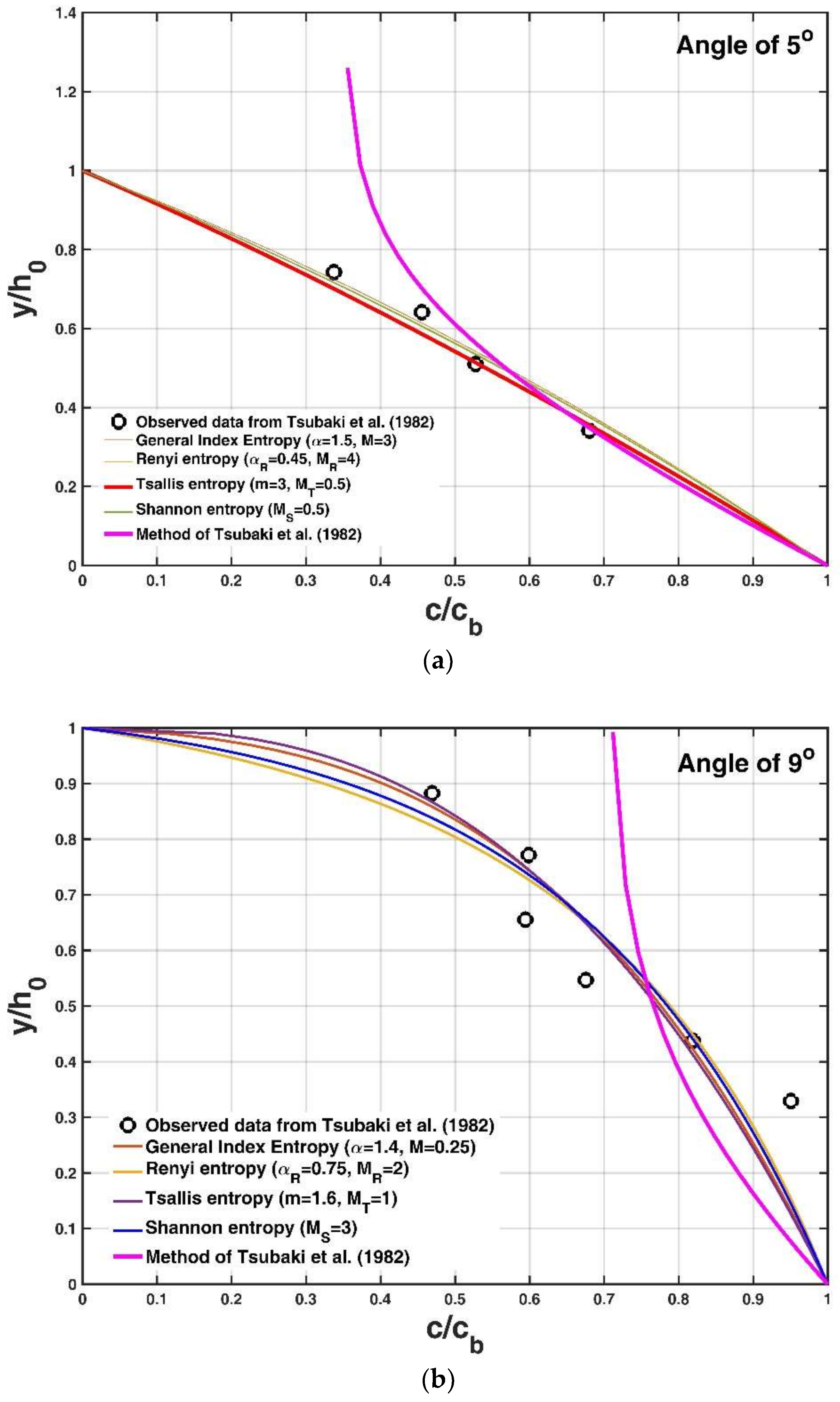
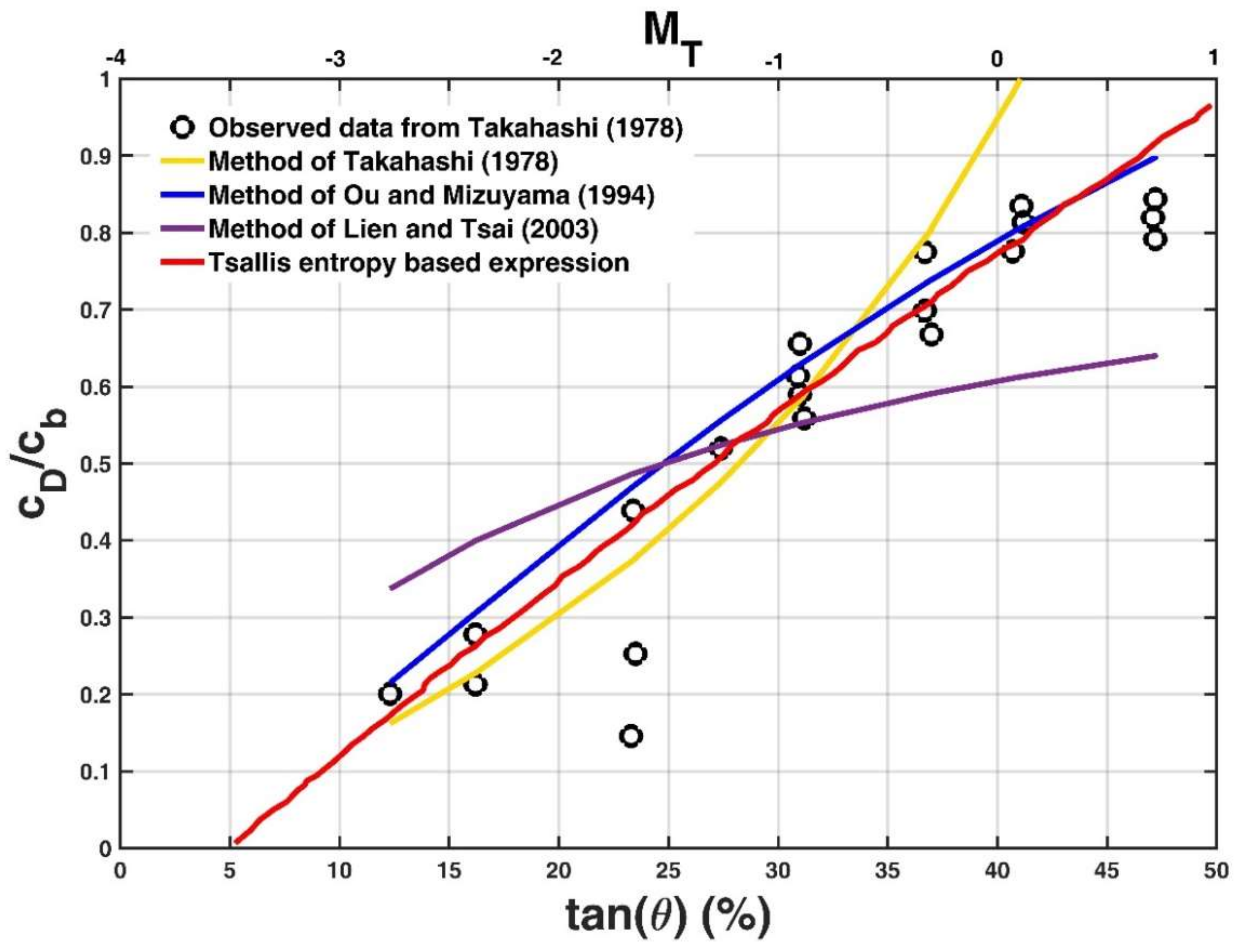
There are very limited experimental data sets regarding sediment concentration in debris flow in the literature, possibly because of difficulty in measuring and detecting sediment concentration [4,5,6]. In this study, only the experimental data regarding the distribution of sediment concentration in debris flow from Tsubaki et al. [18] were adopted to test the validity of the conventional method (Equation (1)) and four entropy-based expressions (Equations (22), (35), (41), and (47)). Tsubaki et al. [18] conducted an experiment of debris flow movement in a 7-m-long and 15-cm-wide flume with angles of 5° and 9° (that is, the angle of inclination of the channel bed from the horizontal line). Mesalite was adopted as a bed material in the experiment. Its density, ${\rho }_s$, was 1600 kg/m³, and the angle of internal friction, $\varphi$, was 38°. The sediment concentration in the experiment was measured over the entire depth of the flow using a camera and an imaging system via the transparent sidewall of the flume. In this experiment, the bed sediment concentration, $c_b$, was 0.59. More experimental details can be found in the work of Tsubaki et al. [18]. For the mean sediment concentration in debris flow, the observed data from the laboratory experiment by Takahashi [8] were adopted in this study to test the validity of three conventional deterministic methods (Equations (5)–(7)) and four entropy-based expressions (Equations (23), (36), (42), and (48)) due to the limited experimental data from the literature. In the experiment by Takahashi [8], where $\tan \varphi$ = 0.75, the density of particles, ${\rho }_s$, was 2600 kg/m³, and the bed sediment concentration, $c_b$, was 0.756. By tilting the board, different values of the inclination angle of the channel bed from the horizontal $\theta$ were generated for observing changes in $c_D$. More information regarding the experiment can be found in the work of Takahashi [8].

To measure the accuracy of the developed expressions with collected experimental data sets, an error analysis was carried out in this study by computing the average value of the relative error, $R$, (in percentage) as follows:

$$R=\frac{100}{N}\left[{\displaystyle {\sum }_{i=1}^N\left|\frac{m_i-o_i}{o_i}\right|}\right]$$

(49)

where $m$ and $o$ are the calculated and observed points, respectively, and $N$ is the number of observed data points. The goodness of fit increases when the $R$ value decreases.

4.2. Comparison Results

Figure 2a,b compares the method of Tsubaki et al. [18] (Equation (1)), the general index entropy-based expression (Equation (22)), the Renyi entropy-based expression (Equation (35)), the Tsallis entropy-based expression (Equation (41)), and the Shannon entropy-based expression (Equation (47)) with observed data from Tsubaki et al. [18] at angles of 5° and 9°.

Table 1. Fitting results of the method of Tsubaki et al. [18] and four different entropy-based expressions for observed data from Tsubaki et al. [18] at angles of 5° and 9°.

Name	Inclination Angle of 5°		Inclination Angle of 9°
	Fitting Coefficient Values	Fitting Result	Fitting Coefficient Values	Fitting Result
		$\mathit{R}$		$\mathit{R}$
Theoretical formula of Tsubaki et al. [18]	No	10.41	No	-
General index entropy-based expression	$\alpha$ = 1.5, $M$ = 3	5.95	$\alpha$ = 1.4, $M$ = 0.25	7.70
Renyi entropy-based expression	${\alpha }_R$ = 0.45, $M_R$ = 4	6.55	${\alpha }_R$ = 0.75, $M_R$ = 2	10.86
Tsallis entropy-based expression	$m$ = 3, $M_T$ = 0.5	7.09	$m$ = 1.6, $M_T$ = 1	7.09
Shannon entropy-based expression	$M_S$ = 0.5	6.51	$M_S$ = 3	9.46

The symbol “-” indicates that the developed expression did not fit the experimental data.

presents the comparisons (the calculated $R$ value) for each case as well as the fitting coefficient values of the four entropy-based expressions.

It can be seen from Figure 2a and Table 1 that the method of Tsubaki et al. [18] greatly deviated from the observed data, whereas all four entropy-based expressions had a better fitting effect. The general index entropy-based expression approached the Renyi entropy-based expression and Shannon entropy-based expression. The general index entropy-based expression had the least error ($R$ = 5.95). The Tsallis entropy-based expression also fitted the data well, with $R$ = 7.09.

It can be seen from Figure 2b and Table 1 that the theoretical formula of Tsubaki et al. [18] did not fit the observed data well. The general index entropy-based expression and the Tsallis entropy-based expression had a better fitting result than the other two entropy expressions. Among these expressions, the Tsallis entropy-based expression had the best agreement with the data sets ($R$ = 7.09).

Figure 3 compares the formulae of Takahashi [8] (Equation (5)), Ou and Mizuyama [19] (Equation (6)), and Lien and Tsai [12] (Equation (7)) and the Tsallis entropy-based expression (Equation (42)) with the observed data of the mean sediment concentration in debris flow from Takahashi [8]. In this figure, the general index entropy-based expression (Equation (23)), Renyi entropy-based expression (Equation (36)), and Shannon entropy-based expression (Equation (48)) are not shown because they did not fit the data points well.

Table 2. Fitting results of the formulae of Takahashi [8], Ou and Mizuyama [19], and Lien and Tsai [12] and the Tsallis entropy-based expression with observed data of sediment concentration in debris flow from Takahashi [8].

Name	Fitting Coefficient Values	Fitting Result R
Formula of Takahashi [8]	No	30.83
Formula of Ou and Mizuyama [19]	No	27.07
Formula of Lien and Tsai [12]	$\eta$ = 0.15	37.99
Tsallis entropy-based expression	$m$ = 3	19.31

presents the fitting results (the calculated $R$ value) for each case. The value of $\eta$ = 0.15 was obtained after fitting Equation (7) to the data points, and $m$ = 3 was presented in Singh and Cui [13]. Note that the Tsallis entropy-based expression (Equation (42)) was not related to the angle $\theta$. Thus, this expression is plotted versus a secondary horizontal axis, $M_T$, in Figure 3. It can be seen from this figure as well as Table 2 that the relationship between $\frac{c_D}{c_b}$ and $M_T$ by the Tsallis entropy-based expression provided the best fit to the observed data points for different $\theta$ values in comparison to the formulae of Takahashi [8], Ou and Mizuyama [19], and Lien and Tsai [12], even though it is not related to the angle $\theta$, as also shown in Singh and Cui [13]. The range of variation of the angle $\theta$ linearly corresponds to the range of variation of $M_T$ from −3 to 1. This result seems to imply that the nondimensional entropy parameter, $M_T$, in the Tsallis entropy-based expression is related to the inclination of the channel bed from the horizontal line.

These results show the potential of the Tsallis entropy theory together with the principle of maximum entropy as a good addition to existing conventional deterministic methods to predict the sediment concentration in debris flow over a channel. These expressions have a simple mathematical form and contain fewer parameter inputs compared with conventional deterministic models. The distribution of sediment concentration and the mean sediment concentration in debris flow can be estimated easily using Equations (41) and (42) as long as the nondimensional entropy parameter is given. However, it should be noted that the entropy method contains fewer physical properties than conventional deterministic models. For example, the angle, $\theta$, of inclination of the channel bed from the horizontal line plays an important role in promoting the movement of debris flow over the channel. The quantity $\tan \theta$ exists in conventional deterministic models; however, it cannot be incorporated in entropy-based expressions.

5. Concluding Remarks

This study derived the analytical expressions for the distribution of sediment concentration and the mean sediment concentration in debris flow using the general index entropy and Renyi theories together with the principle of maximum entropy developed by Jaynes and tested the validity of existing conventional deterministic methods and four different entropy-based expressions. The entropy-based expressions were based on the general index entropy, Renyi entropy, Tsallis entropy, and Shannon entropy theories. The collected observed data sets originated from Tsubaki et al. [18] and Takahashi [8], considering that there is very limited experimental data in the literature.

Comparing the theoretical formula of Tsubaki et al. [18] and four different entropy-based expressions with two observed data sets of Tsubaki et al. [18], it was found that the entropy-based expression agreed with the data better than the conventional method. In particular, the general index entropy and the Tsallis entropy-based expressions were found to have a good fitting result.

Comparing the formulae of Takahashi [8], Ou and Mizuyama [19], and Lien and Tsai [12] as well as four different entropy-based expressions with the observed data of Takahashi [8], it was found that the entropy-based expressions, except the Tsallis entropy, did not fit the data well. In contrast, the Tsallis entropy-based expression had the highest prediction accuracy for the data sets in comparison to conventional deterministic methods. This study shows the potential of using the Tsallis entropy theory together with the principle of maximum entropy to predict sediment concentration in debris flow over an erodible channel bed.

References

- Kang, S.; Lee, S.R. Debris flow susceptibility assessment based on an empirical approach in the central region of South Korea. Geomorphology 2018, 308, 1–12. [Google Scholar] [CrossRef]
- Wei, Z.L.; Xu, Y.P.; Sun, H.Y.; Xie, W.; Wu, G. Predicting the occurrence of channelized debris flow by an integrated cascading model: A case study of a small debris flow-prone catchment in Zhejiang Province, China. Geomorphology 2018, 308, 78–90. [Google Scholar] [CrossRef]
- Zhang, N.; Matsushima, T. Numerical investigation of debris materials prior to debris flow hazards using satellite images. Geomorphology 2018, 308, 54–63. [Google Scholar] [CrossRef]
- Zhang, N.; Matsushima, T. Simulation of rainfall-induced debris flow considering material entrainment. Eng. Geol. 2016, 214, 107–115. [Google Scholar]
- Yu, B.; Yang, Y.H.; Su, Y.C.; Wang, G.F. Research on the giant debris flow hazards in Zhouqu county, Gansu Province on August 7, 2010. J. Eng. Geol. 2010, 4, 437–444. [Google Scholar]
- Tang, C.; Rengers, N.A.; Th, WJ.; Yang, Y.H.; Wang, G.F. Triggering conditions and depositional characteristics of a disastrous debris flow event in Zhouqu city, Gansu province, northwestern China. Nat. Hazards Earth Syst. Sci. 2011, 11, 2903–2912. [Google Scholar] [CrossRef]
- Wang, F.W.; Wu, Y.H.; Yang, H.F.; Tanida, Y.; Kamei, A. Preliminary investigation of the 20 August 2014 debris flows triggered by a severe rainstorm in Hiroshima City, Japan. Geoenviron. Disasters 2015, 2, 1–17. [Google Scholar] [CrossRef]
- Takahashi, T. Mechanical characteristics of debris flow. J. Hydraul. Div. Am. Soc. Civ. Eng. 1978, 104, 1153–1169. [Google Scholar]
- Kappes, M.S.; Malet, J.P.; Remaitre, A.; Horton, P.; Jaboyedoff, M.; Bell, R. Assessment of debris-flow susceptibility at medium-scale in the Barcelonnette Basin, France. Nat. Hazards Earth Syst. Sci. 2011, 11, 627–641. [Google Scholar] [CrossRef]
- Chen, H.; Lee, C. Numerical simulation of debris flows. Can. Geotech. J. 2000, 37, 146–160. [Google Scholar] [CrossRef]
- Rickenmann, D.; Zimmermann, M. The 1987 debris flows in Switzerland: Documentation and analysis. Geomorphology 1993, 8, 175–189. [Google Scholar] [CrossRef]
- Lien, H.P.; Tsai, F.W. Sediment concentration distribution of debris flow. J. Hydraul. Eng. 2003, 129, 995–1000. [Google Scholar] [CrossRef]
- Singh, V.P.; Cui, H.J. Modelling sediment concentration in debris flow by Tsallis entropy. Phys. A 2015, 420, 49–58. [Google Scholar] [CrossRef]
- Jaeger, H.M.; Nagel, S.R. Physics of the granular state. Science 1992, 255, 1523–1530. [Google Scholar] [CrossRef] [PubMed]
- Li, Y.; Zhou, X.J.; Su, P.C.; Kong, Y.D.; Liu, J.J. A scaling distribution for grain composition of debris flow. Geomorphology 2013, 192, 30–42. [Google Scholar]
- Zhang, R.J. River Sediment Dynamics; China Water & Power Press: Beijing, China, 2008. [Google Scholar]
- Fei, X.J.; Shu, A.P. Movement Mechanism of Debris Flow and Disaster Prevention; Tsinghua University Press: Beijing, China, 2004. [Google Scholar]
- Tsubaki, T.; Hashimoto, H.; Suetsugi, T. Grain stresses and flow properties of debris flow. Proc. Jpn. Soc. Civ. Eng. 1982, 317, 79–91. (In Japanese) [Google Scholar] [CrossRef]
- Ou, G.; Mizuyama, T. Predicting the average sediment concentration of debris flow. J. Jpn. Erosion Control Eng. Soc. 1994, 47, 9–13. (In Japanese) [Google Scholar]
- Shorrocks, A.F. The class of additively decomposable inequality measures. Econometrica 1980, 48, 613–614. [Google Scholar] [CrossRef]
- Singh, V.P.; Sivakumar, B.; Cui, H.J. Tsallis entropy theory for modelling in water engineering: A review. Entropy 2017, 19, 641. [Google Scholar] [CrossRef]
- Jaynes, E.T. Information theory and statistical mechanics I. Phys. Rev. 1957, 106, 620–630. [Google Scholar] [CrossRef]
- Jaynes, E.T. Information theory and statistical mechanics II. Phys. Rev. 1957, 108, 171–190. [Google Scholar] [CrossRef]
- Jaynes, E.T. On the rationale of maximum entropy methods. Proc. IEEE 1982, 70, 939–952. [Google Scholar] [CrossRef]
- Kumbhakar, M.; Ghoshal, K. One-dimensional velocity distribution in open channels using Renyi entropy. Stochastic. Environ. Res. Risk Assess. 2017, 31, 949–959. [Google Scholar] [CrossRef]
- Tsallis, C. Possible generalization of Boltzmann–Gibbs statistics. J. Stat. Phys. 1988, 52, 479–487. [Google Scholar] [CrossRef]
- Shannon, C.E. The mathematical theory of communications, I and II. Bell Syst. Tech. J. 1948, 27, 379–423. [Google Scholar] [CrossRef]
Figure 1.
Schematic of steady and uniform debris flow.
Figure 2.
Comparison of the method of Tsubaki et al. [18] (Equation (1)), the general index entropy-based expression (Equation (22)), the Renyi entropy-based expression (Equation (35)), the Tsallis entropy-based expression (Equation (41)), and the Shannon entropy-based expression (Equation (47)) with observed data from Tsubaki et al. [18] at angles of (a) 5° and (b) 9°.
Figure 3.
Comparison of the formulae of Takahashi [8] (Equation (5)), Ou and Mizuyama [19] (Equation (6)), and Lien and Tsai [12] (Equation (7)) and the Tsallis entropy-based expression (Equation (42)) with observed data from Takahashi [8]. Here, the general index entropy-based expression (Equation (23)), the Renyi entropy-based expression (Equation (36)), and the Shannon entropy-based expression (Equation (48)) are not shown because they did not fit the data points completely.