Comparison of Flow-Dependent Controllers for Remote Real-Time Pressure Control in a Water Distribution System with Stochastic Consumption

Abstract

The control of pressure at a remote critical node using a pressure control valve is a highly effective way to attain pressure management. To perform real-time control, various kinds of controllers can be used, including flow-dependent controllers. These controllers calculate valve setting adjustment based both on the deviation of the pressure from the set-point and on the flow rate at the valve site. After putting all the flow-dependent controllers present in the scientific literature within the same framework, this paper presents a numerical comparison of their performance under realistic conditions of stochastic demand. Two controllers were selected for the comparison, namely the simple LCF (parameter-less proportional controller with known constant pressure control valve flow); and LVF (parameter-less controller with known variable pressure control valve flow), which uses a flow rate forecast. Indeed, this study considered an upgrade of LVF, in which the flow rate forecast was tailored to the conditions of stochastic demand. The application in a specific example network proved the performance of these controllers to be quite similar, although LCF was preferable due to its simple structure. For LCF, the average pressure at the critical node had a clear relationship to the consumption pattern. LVF outperformed when the hourly variation dominates the fluctuations in the flow. The conditions under which this out-performance occurred are comprehensively discussed.

1. Introduction

Decreased pressure reduces water leakage from pipes, lowers pipe burst frequency and may reduce water consumption [1]. The device that is by far the most widely used to reduce pressure in a water distribution system (WDS) is a pressure control valve (PCV): commonly a pressure reducing valve (PRV) [2,3].

A closed-loop technique uses measurements in the WDS, while an open-loop technique does not. Earlier advanced pressure management techniques, with the first being the simplest, include: (1) time modulation (open-loop) [1]; (2) flow modulation (closed-loop) [4,5]; and (3) remote node modulation, which is not real-time (closed-loop) [6]. These earlier techniques reduce the pressure better than a classical PCV with no controller, but do not reduce the pressure as low as possible.

A WDS node where the pressure is sensitive to PCV adjustment, and whenever possible, also has the lowest pressure, is called a critical node (CN) [7]. To keep the pressure at the CN continually constant [8], the PCV setting must be changed in real-time, i.e., not manually, intermittently or only at specific times. This is usually accomplished by adjusting the setting every time-step, where the time-step is typically of the order of minutes [7].

The remote real-time control (RRTC) technique strives to make the pressure throughout the WDS as low as possible [9,10], by attempting to set the pressure at a remote CN in real-time to a low and constant target set-point value [11,12]. This is made possible by recent advances in the availability of wireless technology [13,14,15].

A laboratory experiment demonstrated how RRTC with a PRV can be attained by use of a controller [16]. An example of a field demonstration is the one in the district of Benevento, Italy [10].

The controllers in [7,17,18] only use the pressure measurement at the CN. Controllers that also use the flow rate through the PCV, taking changes in WDS conditions into account, were subsequently developed [19,20,21,22,23]. The water flow rate in a pipe equipped with the PCV needs to be measured.

Consumption in a real WDS is stochastic in nature. Recently, several numerical RRTC studies take this into account: either approximating it as random fluctuations [18], or using a comprehensive bottom-up approach [22,23]. This paper reports numerical results on two closely related flow-dependent PCV controllers in the latter approach. One of these was formulated and studied for the first time with stochastic consumption, because this may critically affect the controller’s viability.

2. Head-Loss Controller

In this and the next section, a derivation of various controllers, outlining assumptions made, is presented. This is done in an effort to bring them all together and to put them in the same rigorous framework. The aim is to emphasise that the controllers are important from the viewpoint of hydraulic theory. Particularly, the derivation is within the context of a WDS where there is not significant time-dependence on a time-scale shorter than the control time-step $T_c$, or on a time-scale of a few $T_c$ (see Appendix A).

Let $\tilde{H}$ be the head-loss across the PCV, and H the head at the CN. It can be argued from the Newton–Raphson numerical method (see Appendix A) that an appropriate controller, called the “head-loss” controller [21], would calculate the adjusted head-loss

$${\tilde{H}}_{i+1}={\tilde{H}}_i-S_i(H_i-H_{sp})$$

(1)

from the current head-loss ${\tilde{H}}_i$. Here, $H_{sp}$ is the target set-point head of the CN; and the notation and sensitivity $S_i$ are defined in Appendix A (see also [24]). The information at iteration i determines the next iteration $i+1$. The iterations are separated by $T_c$. The value of $S_i$ varies for different iterations, and is impractical to determine for a real-world WDS without a hydraulic model [21]. When the CN head depends very sensitively on the PCV head-loss, $S_i=-1$ for a PRV. Using this value in Equation (1) yields the controller employed in [9,11,20].

Equation (1) represents the choice of controller, from the viewpoint of theory [12,19,21,23]. However, the controller evaluates hydraulic quantities at a specific time, and hence is not sensible for quantities that exhibit significant time-dependence.

3. Controllers Based on Known PCV Flow Rate

A PCV is conventionally modelled by [17,19,20]:

$$\tilde{H}=\frac{\xi }{2g}{v}^{2}v=\frac{Q}{A}$$

(2)

where $\xi$ is the (dimension-less) PCV head-loss coefficient, v is the water velocity, Q is the flow rate through the PCV, A is the area of the port opening within the PCV, and g is the acceleration due to gravity. Substituting Equation (2) into Equation (1) implies that the adjusted head-loss coefficient can be calculated as

$${\xi }_{i+1}={\xi }_i{\left(\frac{v_i}{v_{i+1}}\right)}^2-\frac{2g{S}_i}{v_{i+1}^2}(H_i-H_{sp})$$

(3)

from the current head-loss coefficient ${\xi }_i$. Equation (3) can be used as the very general form of a controller, as conceived in [23] for $S_i=-1$. It is called the “general parameter-less controller with known variable PCV flow” (GVF). It is parameter-less, because it contains no tunable parameter. Specifically, $S_i$ is not tunable.

The right hand side of Equation (3) is separated into two parts. The first part does not involve the future (does not depend on $v_{i+1}$), and is important because it does not require modelling the future. The second part is the remainder (denoted by $\mathsf{\Phi }$ and $\mathsf{\Psi }$). Separating Equation (3) into these parts yields

$${\xi }_{i+1}={\xi }_i-\frac{2g{S}_i}{v_i^2}(H_i-H_{sp})+{\mathsf{\Phi }}_i+{\mathsf{\Psi }}_i$$

(4)

where

$${\mathsf{\Phi }}_i=-{\xi }_i{f}_i{\mathsf{\Psi }}_i=\frac{2g{S}_i}{v_i^2}{f}_i(H_i-H_{sp})f_i=1-\frac{1}{{\left(1+\frac{\mathsf{\Delta }{v}_i}{v_i}\right)}^2}$$

(5)

with $\mathsf{\Delta }{v}_i\equiv v_{i+1}-v_i$. All dependence on the future in the remainder part is through the dimensionless $f_i$, and hence through $\mathsf{\Delta }{v}_i$, which needs to be modelled.

Neglecting $\mathsf{\Delta }{v}_i$ leads to a controller with

$${\mathsf{\Phi }}_i\approx 0{\mathsf{\Psi }}_i\approx 0$$

(6)

Equations (4) and (6) define the “parameter-less proportional controller with known constant PCV flow” (LCF) [21]. With $S_i=-1$, it is first derived in [19]; and is also called “valve resistance” (RES) control [11,20].

Another controller can be obtained by only keeping the dominant terms in $\mathsf{\Phi }$ and $\mathsf{\Psi }$, which are linear and up to first order in the difference terms. $f_i$ is proportional to $\mathsf{\Delta }{v}_i$. Hence, ${\mathsf{\Psi }}_i$ is the only term in Equation (4) that is proportional to two difference terms ($\mathsf{\Delta }{v}_i$ and $H_i-H_{sp}$) and can accordingly be neglected. $f_i$ can be evaluated to lowest order in the difference term $\mathsf{\Delta }{v}_i$, leading to a controller with

$${\mathsf{\Phi }}_i\approx -\frac{2{\xi }_i}{v_i}\mathsf{\Delta }{v}_i{\mathsf{\Psi }}_i\approx 0$$

(7)

Equations (4) and (7) define the “parameter-less controller with known variable PCV flow” (LVF), first derived in [21].

4. Modification of Controllers: Stochastic Consumption

In a real WDS, there is usually significant time-dependent behaviour due to stochastic water consumption. For this situation, the controllers need to be modified, so that a hydraulic quantity evaluated at a specific time is postulated to be replaced by an average. Let $Z(t_{i-n},t_i)$ be the average of Z in the time interval from $t_{i-n}=t_i-n{T}_c$ to $t_i$. Then, it is natural to define the controllers in Equations (3)–(7) to be used with $H_i$ and $v_i$ replaced by $H(t_{i-1},t_i)$ and $v(t_{i-1},t_i)$, respectively, as done in [11,22] for the LCF controller with $S_i=-1$. Similarly, $S_i$ is replaced by $S(t_{i-1},t_i)$.

The future change $\mathsf{\Delta }{v}_i$ can be modelled by estimating it from the past. Since $\mathsf{\Delta }{v}_i$ is a velocity change in an interval $T_c$, it is proposed that it should be replaced in Equation (7) by

$$\frac{v(t_{i-n},t_i)-v(t_{i-2n},t_{i-n})}{n}$$

(8)

Hence, n is an indicator of how far back the past mean values are used to predict the future. For each n, the corresponding LVF controller is denoted LVFn.

5. Numerical Study in the Example WDS

Controllers LCF and LVF were applied to the RRTC of a network in northern Italy (see skeletonised layout in Figure 1), which caters to about 30,000 inhabitants. This network has already been used for investigations in the area of pressure management [19,22,25].

The network consists of a single source node (node 27), although networks with more sources could also be considered. There are 26 demanding nodes with ground elevation of 0 m a.s.l. and 32 pipes. The network can be considered as a single pressure zone, because of its size and the uniform ground elevation.

The references above give further details about the characteristics of the network. The source node has a head varying around 40 m a.s.l. [22]. A single DN300 plunger valve is the PRV, located at the end of pipe 26-11. The PRV has the head-loss coefficient $\xi \left(\alpha \right)$ given by

$$\xi ={10}^{c_1-c_2{log}_{10}(1-\alpha )}$$

(9)

where data from the valve manufacturer allow the coefficients $c_1=1.5$ and $c_2=2.8$ to be calculated. The setting $\alpha$ is adjusted by the controller; and is constrained to range from 0 (completely open) to 0.95 (nearly completely closed). The maximum value $\alpha =0.95$ was chosen consistent with the real use of control valves, the objective of which is to modulate flow, rather than to interrupt it. However, it must be noted that this upper boundary does not affect the results of the simulations, as shown below.

The lowest pressure values during the day are found at node 1, which was hence selected as the CN where pressure control was applied. The RRTC of the PCV was performed to enable the pressure head at the CN to be near the target set-point head of $H_{sp}=25$ m.

The bottom-up approach detailed in [22,25] was used to obtain the consumption for each node. This approach is based on consumption pulse generation through the Poisson model [26], considering pulse duration and intensity to be dependent random variables, both of which are expressed through the beta distribution. The pulse arrival rate at each node was calculated to obtain the expected average nodal demand, while considering the pattern of total demand observed in the WDS in a single day. More details of the bottom-up approach for demand generation are presented in [22], along with the parameter values used for demand generation.

To describe the hydraulics of the WDS, the model described in [22] was used. This model enables the unsteady flow modelling of the WDS and the accurate reproduction of the hydraulic behaviour of the valve. Compared to other software available in the market, this proprietary model has the advantage of considering unsteady flow pipe resistances, thus yielding more realistic results.

6. Results

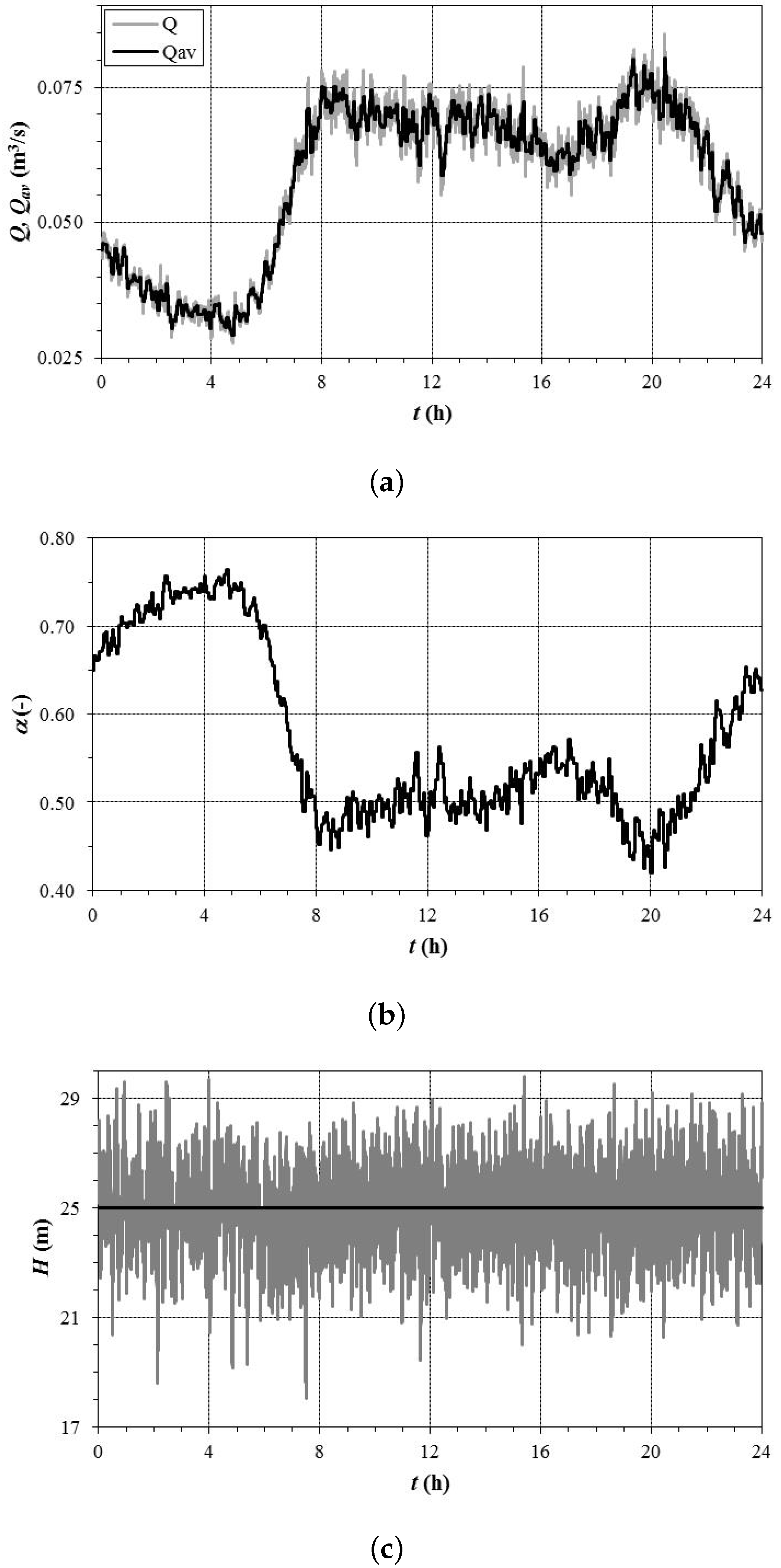
Since preliminary investigations proved that $S_i=-1$ gave good results, this value was kept throughout all the calculations. As an example of the results, Figure 2 reports calculations over a day for LCF with $T_c=3$ min. The instantaneous and averaged flow-rate $Q_{av}$ through the PCV, valve setting and instantaneous pressure at the CN are shown. As for the flow-rates, these values include the WDS pulsed demand [22] (Figure 4) and leakage, which added up on average to approximately 20% of the total output from the source. As for the valve setting, it must be noted that it always stayed far from the lower and upper boundaries, attesting to the proper regulation behaviour of the valve.

The LVF controller models the future from the past. All LVFn controllers that use velocities for a period $2n{T}_c\le 42$ min into the past were investigated. A different method from Equation (8), which uses a regression fit of past $Q_{av}$ values to predict the future flow, has also been proposed [23].

Let ${\left|e\right|}_{mean}$ and $e_{mean}$ denote the average of $|H-H_{sp}|$ and $H-H_{sp}$, respectively, where H is evaluated every second. These two performance measures determine the deviation of the pressure at the CN from the target set-point. In accordance with [22], the primary measure was ${\left|e\right|}_{mean}$. In addition, let the performance measure $\mathsf{\Sigma }\left|\mathsf{\Delta }\alpha \right|$ be the sum of the actuator setting absolute corrections evaluated at each iteration. This is a measurement of the wear and tear on the PCV due to setting changes. Performance is the best when the performance measures are as low as possible.

Undesirable behaviour due to PRV self-interactions was observed for $T_c\le 1$ min [22], thus $T_c=3,5$ and 10 min were considered. Of the time-steps studied, $T_c=3$ min gave the lowest ${\left|e\right|}_{mean}$ for both LCF and LVF. The results for the full 24-h period with this time-step are now discussed.

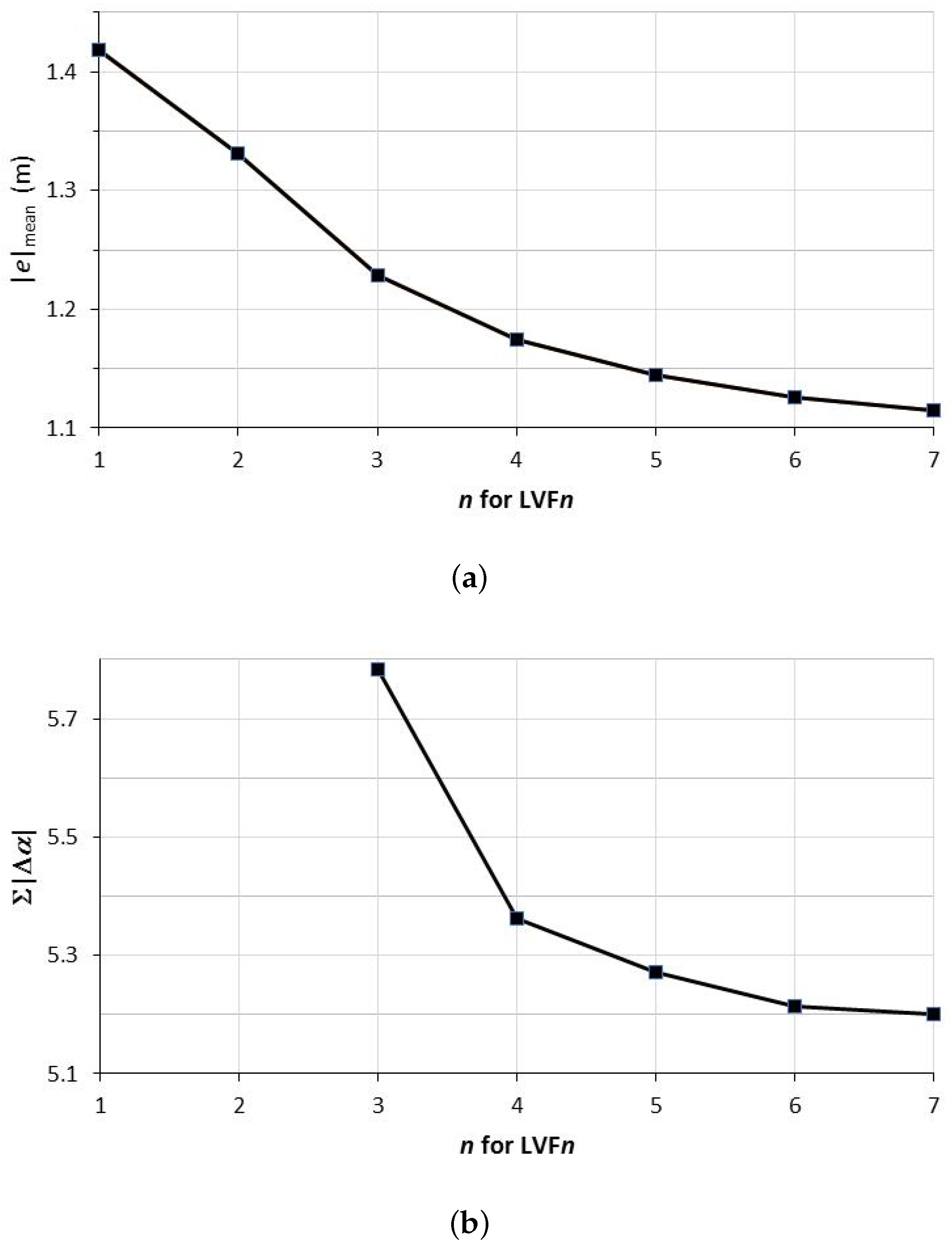
For LVFn, ${\left|e\right|}_{mean}$ and $\mathsf{\Sigma }\left|\mathsf{\Delta }\alpha \right|$ decreased monotonically as n increased (Figure 3). Evidently, decreases became insignificant nearing $n=7$. It was also found that this monotonic decrease happened in each individual hourly period. The best performing LVFn was hence LVF7, which uses velocities for a period 42 min into the past. However, ${\left|e\right|}_{mean}$ and $\mathsf{\Sigma }\left|\mathsf{\Delta }\alpha \right|$ were perfectly reasonable for LVF3, if a controller looking less into the past were desired.

For the day, ${\left|e\right|}_{mean}$(LVF)$-{\left|e\right|}_{mean}$(LCF) $=0.016$ m, thus LCF outperformed insignificantly. Evaluating a similar difference for $\mathsf{\Sigma }\left|\mathsf{\Delta }\alpha \right|$, it was found that LCF outperformed LVF7 by a tiny 0.85%.

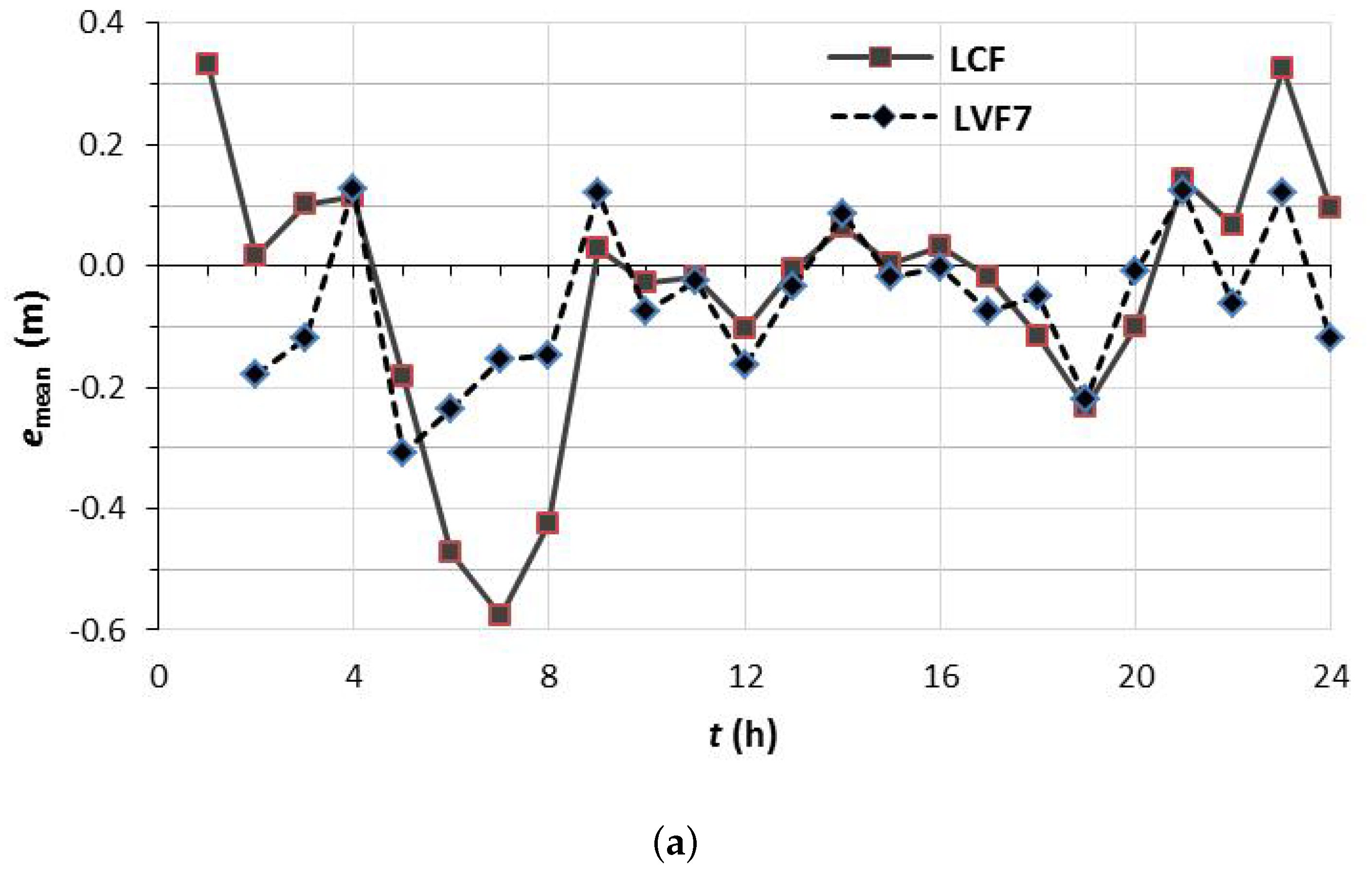
It is interesting to determine the variation of the pressure deviation during the day. Comparison with the consumption pattern can more easily be done by evaluating hourly averages, in order to reduce the effect of stochastic fluctuation in consumption. In Figure 4, ${\left|e\right|}_{mean}$ is shown as a function of time. It is noticeable that the results for LCF and LVF7 are very similar at a certain time, and that there is apparently random variation from hour to hour. This suggests that ${\left|e\right|}_{mean}$ has significant stochastic fluctuation. On the other hand, $e_{mean}$ as a function of time shows clear patterns (especially for LCF), and appears to be less dependent on stochastic fluctuation (Figure 5a).

Assume that the flow rate through the PCV in Figure 2a is fitted by a smoothly varying $Q_{trend}$, which indicates the trend in the flow rate (the hourly variation). The results for LCF in Figure 5a have an interesting pattern. $Q_{trend}$ increased noticeably during 5–8 h and 17–20 h. Accordingly, $e_{mean}$ was negative for the points in Figure 5a representing these hours. In addition, the deviation of $e_{mean}$ from zero was largest for the period 6–7 h when the rate of change of flow was the largest of the entire day. The flow decreased noticeably during 0–1 h and 20–24 h. Fittingly, $e_{mean}$ was positive for the points in Figure 5a representing these hours.

All of these observations for LCF were consistent with a related study predicting that the deviation of the pressure is approximately proportional to $-Q^{\prime }/Q$ in the context of non-stochastic consumption [27], where $Q^{\prime }$ is the rate of change of Q.

For non-stochastic consumption, numerical results for LCF were previously pointed out to suggest that the deviation is driven by $-Q^{\prime }$ [21]. This can be confirmed by Figures 7, 10, 12 and 13 of [11], and in the pressure shown in Figure 7 (7-RES) [12]. For stochastic consumption, this behaviour can also be seen in Figure 7b of [22].

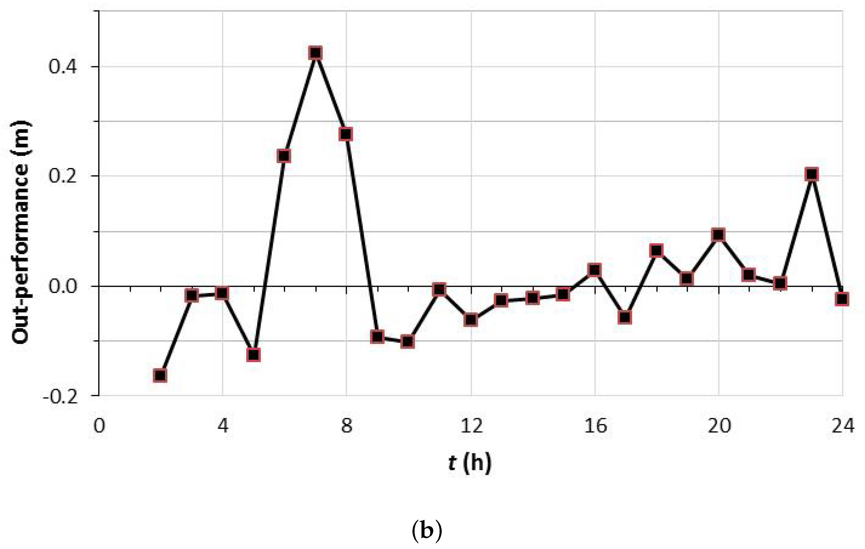
Figure 5a shows that LVF7 was less prone than LCF to deviate significantly from the target set-point pressure. Figure 5b indicates that LVF7 substantially outperformed LCF during Hours 5–8. This coincided with the hours when $Q_{trend}$ changed the most quickly. In addition, during the second fastest flow change during 20–24 h, LVF7 outperformed LCF.

The sum of the out-performance amounts for each hour in Figure 5b was 0.028 m. Hence, with the performance measure $e_{mean}$, LVF7 outperformed LCF insignificantly over the day. Taking into account the results from all three performance measures, it is fair to say that the performance of LVF7 was the same as LCF over the entire day.

7. Discussion

Water consumption shows stochastic fluctuation in a real WDS. There are also unsteady flow processes that can cause sudden variations in flow and pressure [4,5,28]. For RRTC, the effect on a proportional-integral controller of adding random consumption fluctuation at each time-step $T_c$ to smooth water consumption is initially studied in [18]. The bottom-up approach used in this work incorporates both fully stochastic consumption fluctuation and unsteady flow processes.

From the viewpoint of the derivation of the controllers, LVF should at first glance be an improvement on LCF. However, LVF depends on a future change $\mathsf{\Delta }{v}_i$, which can only be modelled by estimating it from the past [11]. The way to decrease the effect of stochastic fluctuation in consumption is to estimate $\mathsf{\Delta }{v}_i$ by looking far into the past (Figure 3). However, relying on the far past is undesirable, as shown by the case of no fluctuation. (Assuming Q is a smooth function of time, estimating $\mathsf{\Delta }{v}_i$ from the most recent past velocities should be the most accurate). Hence, the larger is the fluctuation, the greater is the performance of LVF weakened.

The performance of LVF relative to LCF depends on a large number of factors. For a given WDS, these were argued to include $|Q_{trend}^{\prime }|$ at a certain time. It is postulated that this is to be compared to the magnitude of the average fluctuation at a certain time. The following study indicates what happens if $|Q_{trend}^{\prime }|$ dominates the fluctuations. For non-stochastic consumption, LVF1 was found to strongly outperform LCF at almost all times in two WDSs (Figures 3, 5 and 6 of [27]). In another study, a controller that uses future flow forecasting (LCb [23]) shows a clear advantage above the case when the future forecasting is neglected (LCa), when the fluctuations in consumption are small compared to its hourly variation. The advantage is obtained for a flow rate that has smaller fluctuations and much larger hourly variation than in Figure 2a.

In the current study for $T_c=3$ min, it was found that LVF7 outperformed LCF when $|Q_{trend}^{\prime }|$ was large at a certain time. On the other hand, LVF7 and LCF performed the same during the entire day, for the assumed consumption pattern. However, it is expected that LVFn can outperform over the entire day (for some n) when there are more hours when $|Q_{trend}^{\prime }|$ dominates the fluctuations, or there are hours when $|Q_{trend}^{\prime }|$ strongly dominates the fluctuations.

8. Conclusions

Of the three time-steps considered, 3 min was used because it gave the best performance for the example network and consumption. Extensive care was taken to construct this realistic example, for which the flow-dependent LCF and LVF7 controllers were found to have the same overall performance. However, since LVF7 was more complicated, LCF Was preferable, and should be considered as the controller of choice.

The performance of the LVF controller relative to LCF is expected to be better when:

• The magnitude of the average stochastic fluctuation in consumption decreases.
• There are many hours with a sizeable magnitude of the rate of change of the flow rate through the valve $|Q_{trend}^{\prime }|$.
• There are hours with a large $|Q_{trend}^{\prime }|$.

Unless the factors listed above are particularly favourable, the flow-dependent controller, which does not require modelling the future (LCF here), is an adequate choice with stochastic consumption, even though it may not perform as well as the controller that requires modelling the future (LVF here). This remains true even in the case where it is preferable or necessary to replace the sensitivity with a dimension-less tunable parameter [23].

Further research can address ways to improve controllers that model the future.

References

- Vicente, D.J.; Garrote, L.; Sánchez, R.; Santillán, D. Pressure management in water distribution systems: Current status, proposals, and future trends. J. Water Resour. Plan. Manag. 2015, 142, 04015061. [Google Scholar] [CrossRef]
- Ates, S. Hydraulic modelling of control devices in loop equations of water distribution networks. Flow Meas. Instrum. 2017, 53, 243–260. [Google Scholar] [CrossRef]
- Adedeji, K.B.; Hamam, Y.; Abe, B.T.; Abu-Mahfouz, A.M. Pressure management strategies for water loss reduction in large-scale water piping networks: A review. In Advances in Hydroinformatics; Gourbesville, P., Cungem, J., Caignaert, G., Eds.; Springer Water; Springer: Singapore, 2018; pp. 465–480. [Google Scholar]
- Prescott, S.L.; Ulanicki, B. Improved control of pressure reducing valves in water distribution networks. J. Hydraul. Eng. 2008, 134, 56–65. [Google Scholar] [CrossRef]
- Ulanicki, B.; Skworcow, P. Why PRVs tends to oscillate at low flows. Procedia Eng. 2014, 89, 378–385. [Google Scholar] [CrossRef]
- Bakker, M.; Rajewicz, T.; Kien, H.; Vreeburg, J.H.G.; Rietveld, L.C. Advanced control of a water supply system: A case study. Water Pract. Technol. 2014, 9, 264–276. [Google Scholar] [CrossRef]
- Campisano, A.; Creaco, E.; Modica, C. RTC of valves for leakage reduction in water supply networks. J. Water Resour. Plan. Manag. 2010, 136, 138–141. [Google Scholar] [CrossRef]
- Nicolini, M.; Zovatto, L. Optimal location and control of pressure reducing valves in water networks. J. Water Resour. Plan. Manag. 2009, 135, 178–187. [Google Scholar] [CrossRef]
- Sanz, E.; Pérez, R.; Sánchez, R. Pressure control of a large scale water network using integral action. In Proceedings of the 2nd IFAC Conference on Advances in PID Control, Brescia, Italy, 28–30 March 2012; pp. 270–275. [Google Scholar]
- Fontana, N.; Giugni, M.; Glielmo, L.; Marini, G. Real-time control of pressure for leakage reduction in water distribution network: Field experiments. J. Water Resour. Plan. Manag. 2018, 144, 04017096. [Google Scholar] [CrossRef]
- Giustolisi, O.; Ugarelli, R.M.; Berardi, L.; Laucelli, D.B.; Simone, A. Strategies for the electric regulation of pressure control valves. J. Hydroinform. 2017, 19, 621–639. [Google Scholar] [CrossRef]
- Berardi, L.; Simone, A.; Laucelli, D.B.; Ugarelli, R.M.; Giustolisi, O. Relevance of hydraulic modelling in planning and operating real-time pressure control: Case of Oppegård municipality. J. Hydroinform. 2017, 20, 535–550. [Google Scholar] [CrossRef]
- Campisano, A.; Cabot Ple, J.; Muschalla, D.; Pleau, M.; Vanrolleghem, P.A. Potential and limitations of modern equipment for real time control of urban wastewater systems. Urban Water J. 2013, 10, 300–311. [Google Scholar] [CrossRef]
- Kruger, C.P.; Abu-Mahfouz, A.M.; Hancke, G.P. Rapid prototyping of a wireless sensor network gateway for the Internet of Things using off-the-shelf components. In Proceedings of the 2015 IEEE International Conference on Industrial Technology (ICIT), Seville, Spain, 17–19 March 2015; pp. 1926–1931. [Google Scholar]
- Abu-Mahfouz, A.M.; Hamam, Y.; Page, P.R.; Djouani, K.; Kurien, A. Real-time dynamic hydraulic model for potable water loss reduction. Procedia Eng. 2016, 154, 99–106. [Google Scholar] [CrossRef]
- Fontana, N.; Giugni, M.; Glielmo, L.; Marini, G.; Verrilli, F. Real-time control of a PRV in water distribution networks for pressure regulation: Theoretical framework and laboratory experiments. J. Water Resour. Plan. Manag. 2018, 144, 04017075. [Google Scholar] [CrossRef]
- Campisano, A.; Modica, C.; Vetrano, L. Calibration of proportional controllers for the RTC of pressures to reduce leakage in water distribution networks. J. Water Resour. Plan. Manag. 2012, 138, 377–384. [Google Scholar] [CrossRef]
- Campisano, A.; Modica, C.; Reitano, S.; Ugarelli, R.; Bagherian, S. Field-oriented methodology for real-time pressure control to reduce leakage in water distribution networks. J. Water Resour. Plan. Manag. 2016, 142, 04016057. [Google Scholar] [CrossRef]
- Creaco, E.; Franchini, M. A new algorithm for real-time pressure control in water distribution networks. Water Sci. Technol. Water Supply 2013, 13, 875–882. [Google Scholar] [CrossRef]
- Giustolisi, O.; Campisano, A.; Ugarelli, R.; Laucelli, D.; Berardi, L. Leakage management: WDNetXL pressure control module. Procedia Eng. 2015, 119, 82–90. [Google Scholar] [CrossRef]
- Page, P.R.; Abu-Mahfouz, A.M.; Yoyo, S. Parameter-less remote real-time control for the adjustment of pressure in water distribution systems. J. Water Resour. Plan. Manag. 2017, 143, 04017050. [Google Scholar] [CrossRef]
- Creaco, E.; Campisano, A.; Franchini, M.; Modica, C. Unsteady flow modeling of pressure real-time control in water distribution networks. J. Water Resour. Plan. Manag. 2017, 143, 04017056. [Google Scholar] [CrossRef]
- Creaco, E. Exploring numerically the benefits of water discharge prediction for the remote RTC of WDNs. Water 2017, 9, 961. [Google Scholar] [CrossRef]
- Piller, O.; Elhay, S.; Deuerlein, J.; Simpson, A. Local sensitivity of pressure-driven modeling and demand-driven modeling steady-state solutions to variations in parameters. J. Water Resour. Plan. Manag. 2017, 143, 04016074. [Google Scholar] [CrossRef]
- Creaco, E.; Pezzinga, G.; Savic, D. On the choice of the demand and hydraulic modeling approach to WDN real-time simulation. Water Resour. Res. 2017, 53, 6159–6177. [Google Scholar] [CrossRef]
- Creaco, E.; Farmani, R.; Kapelan, Z.; Vamvakeridou-Lyroudia, L.; Savic, D. Considering the mutual dependence of pulse duration and intensity in models for generating residential water demand. J. Water Resour. Plan. Manag. 2015, 141, 04015031. [Google Scholar] [CrossRef]
- Page, P.R.; Abu-Mahfouz, A.M.; Piller, O.; Mothetha, M.L.; Osman, M.S. Robustness of parameter-less remote real-time pressure control in water distribution systems. In Advances in Hydroinformatics; Gourbesville, P., Cungem, J., Caignaert, G., Eds.; Springer Water; Springer: Singapore, 2018; pp. 449–463. [Google Scholar]
- Piller, O.; van Zyl, J.E. Modeling control valves in water distribution systems using a continuous state formulation. J. Hydraul. Eng. 2014, 140, 04014052. [Google Scholar] [CrossRef]
- Press, W.H.; Teukolsky, S.A.; Vetterling, W.T.; Flannery, B.P. Numerical Recipes in FORTRAN; Cambridge University Press: Cambridge, UK, 1992; p. 355. [Google Scholar]
- Page, P.R.; Abu-Mahfouz, A.M.; Mothetha, M.L. Pressure management of water distribution systems via the remote real-time control of variable speed pumps. J. Water Resour. Plan. Manag. 2017, 143, 04017045. [Google Scholar] [CrossRef]
Figure 1.
Example water distribution system.
Figure 2.
(a) Flow-rate Q every second and its value averaged over 3 min; (b) valve setting (evaluated every 3 min); and (c) ressure head H every second.
Figure 3.
Results for LVFn with min over one day: (a) ; and (b) . For , the values are out of range at and , respectively.
Figure 4.
evaluated during an hour period preceding the time of the datum shown min.
Figure 5.
emean evaluated during an hour period preceding the time of the datum shown (Tc = 3 min): (a) emean; and (b) out-performance of LVF7 over LCF, defined using emean. Out-performance is positive if the emean of LVF7 is nearer to 0 than the emean of LCF.
© 2019 by the authors. Licensee MDPI, Basel, Switzerland. This article is an open access article distributed under the terms and conditions of the Creative Commons Attribution (CC BY) license (http://creativecommons.org/licenses/by/4.0/).
Share and Cite
MDPI and ACS Style
Page, P.R.; Creaco, E. Comparison of Flow-Dependent Controllers for Remote Real-Time Pressure Control in a Water Distribution System with Stochastic Consumption. Water 2019, 11, 422. https://doi.org/10.3390/w11030422
AMA Style
Page PR, Creaco E. Comparison of Flow-Dependent Controllers for Remote Real-Time Pressure Control in a Water Distribution System with Stochastic Consumption. Water. 2019; 11(3):422. https://doi.org/10.3390/w11030422
Chicago/Turabian StylePage, Philip R., and Enrico Creaco. 2019. "Comparison of Flow-Dependent Controllers for Remote Real-Time Pressure Control in a Water Distribution System with Stochastic Consumption" Water 11, no. 3: 422. https://doi.org/10.3390/w11030422
Note that from the first issue of 2016, this journal uses article numbers instead of page numbers. See further details here.