Blue Water in Europe: Estimates of Current and Future Availability and Analysis of Uncertainty


1
Department of Civil Engineering: Hydraulics, Energy and Environment, Universidad Politécnica de Madrid, Madrid 28040, Spain
2
Department of Agricultural Economics & CEIGRAM, Universidad Politécnica de Madrid, Madrid 28040, Spain
*
Author to whom correspondence should be addressed.
Water 2019, 11(3), 420; https://doi.org/10.3390/w11030420
Submission received: 29 December 2018
/
Revised: 19 February 2019
/
Accepted: 21 February 2019
/
Published: 26 February 2019
(This article belongs to the Special Issue Water Resources Management Models for Policy Assessment)
Abstract
:This study presents a regional assessment of future blue water availability in Europe under different assumptions. The baseline period (1960 to 1999) is compared to the near future (2020 to 2059) and the long-term future (2060 to 2099). Blue water availability is estimated as the maximum amount of water supplied at a certain point of the river network that satisfies a defined demand, taking into account specified reliability requirements. Water availability is computed with the geospatial high-resolution Water Availability and Adaptation Policy Assessment (WAAPA) model. The WAAPA model definition for this study extends over 6 million km2 in Europe and considers almost 4000 sub-basins in Europe. The model takes into account 2300 reservoirs larger than 5 hm3, and the dataset of Hydro 1k with 1700 sub-basins. Hydrological scenarios for this study were taken from the Inter-Sectoral Impact Model Inter-Comparison Project and included simulations of five global climate models under different Representative Concentration Pathways scenarios. The choice of method is useful for evaluating large area regional studies that include high resolution on the systems´ characterization. The results highlight large uncertainties associated with a set of local water availability estimates across Europe. Climate model uncertainties for mean annual runoff and potential water availability were found to be higher than scenario uncertainties. Furthermore, the existing hydraulic infrastructure and its management have played an important role by decoupling water availability from hydrologic variability. This is observed for all climate models, the emissions scenarios considered, and for near and long-term future. The balance between water availability and withdrawals is threatened in some regions, such as the Mediterranean region. The results of this study contribute to defining potential challenges in water resource systems and regional risk areas.
1. Introduction
Water management is challenged by climate change. By the 2070s, the percentage of the surface area under conditions of severe water stress is expected to increase from the current 19% to 35% in central and southern Europe [1]. Populations living under water stress conditions in regions from 17 countries of Western Europe are projected to increase by between 16 and 44 million [2]. It is also predicted that the runoff of certain rivers may diminish by up to 80% during the summers. Reservoirs may lose resources due to a decrease in rainfall and the frequency of droughts will increase. The consensus is that the effect of climate change will also exacerbate precipitation extremes with more pronounced drought and flood periods [3,4,5]. At the same time, future water demand is increasing due to climate and social changes. Higher temperatures lead to increased water demand for irrigation and urban supply, hydroelectric potential of Europe may decrease 6% on average, and between 20 and 50% in the Mediterranean region. Advances in technology efficiency may only affect industrial demand [2]. In the Mediterranean region, impacts of climate change on water will certainly have a large influence on human water security and biodiversity [6]. There are several hundred local studies on the potential impacts of climate change on water resources in the Mediterranean, which apply many different approaches. Although the results are diverse and sometimes contradictory, a common element is that one of the primary impacts of climate change will be a reduction of water availability in the Mediterranean Region [1,2]. Furthermore, several authors showed that Global Climate Models (GCMs) were the main source of uncertainty when assessing the impacts of climate change on hydrologic processes [7,8]. Meanwhile, uncertainty associated with streamflow appeared to be more consistent with precipitation than temperature and showed higher sensitivity to the selection of GCMs than to the Regional Climate Models (RCPs) [9,10].
Water availability focuses on blue water, which is defined as water that runs off the landscape into streams, rivers, reservoirs, and groundwater [11]. However, the term “water availability” includes multiple aspects. A multitude of studies consider water availability to be directly linked to changes in average runoff, estimated as the net difference between precipitation and evapotranspiration [12,13]. In non-altered basins, water availability would be either null or extremely low because it would be determined by long term minimum values of flow. It is clear that hydraulic infrastructure plays an important role in making water available for users, mainly by the regulation and transportation of water resources. Even though the storage-based strategy proved to be very successful in the past [14], expanding infrastructure is not an option to increase availability in many regions due to social and environmental constraints [15]. As a result, increasing demand relies heavily on management. The emphasis is currently being placed on how to improve management of existing infrastructure and on socio-economic measures through demand management and water use efficiency [16,17]. The main factors to be considered in regulated water resource systems are the stream flow variability, storage capacity, and yield reliability. In this study, we define blue water availability as the amount of water that can be supplied at a certain point of the river network to satisfy a regular demand under specified reliability requirements [18,19]. Therefore, water availability is the combined result of natural processes, existing infrastructure, and policy. A wide range of techniques have been proposed to analyse water availability, from relatively simple stochastic processes relating these variables to highly complex models solving the water allocation problem [20,21,22,23,24], even including social and economic considerations [25]. In the water sector, institutions, users, technology, and the economy cooperate to achieve equilibrium between water supply and demand in water resource systems. In order to understand the process of reaching future goals for water under climate change, science has developed a set of tools to understand uncertainty [26,27,28,29], assess future impacts [30,31], and facilitate policy development [1,16,18,32]. However, most studies were developed using detailed water management and planning models, and were applied at the local scale. In systems and situations where limited information is available and regional or continental-scale studies are needed, it is generally better to obtain a global overview of the water supply systems’ performance under different climate and policy scenarios, using simplified regional models rather than carrying out very detailed simulations with conventional models, which require very specific information on water demands and infrastructure [18,33,34]. These continental scale-models are conceived to estimate the maximum water availability and to provide technical and quantitative support to possible water policies in the short and long term. Then, these models and detailed water management and planning models should be considered as complementary tools.
Over forty percent of the total water withdrawal in Europe is used for agriculture. Southern countries use the largest percentages of abstracted water for agriculture. This generally accounts for more than two thirds of total abstraction. In northern member States, levels of water use in agriculture are much smaller, with irrigation being less important but still accounting for more than 30% in some areas [35]. Moreover, if the climate in a given region gets drier and warmer, water availability will decrease, and the issue will be exacerbated by increasing water demand [36]. For example, it is expected that areas of maize grain cultivation will expand up to 30–50% in Europe [37,38,39,40] with increases of up to 50% in net primary productivity in northern European ecosystems, as a result of a longer growing season and higher CO2 concentrations [37]. As the projected impacts on productivity of crops and ecosystems included the direct effects of increased CO2 concentration on photosynthesis, the variation in simulated results attributed to differences between the climate models were, in all cases, smaller than the variation attributed to emissions scenarios [37]. The objective of this study is to estimate future potential blue water availability in Europe and its associated uncertainty, which is induced by emissions scenarios and climate change models. This study first proposes a methodology to conduct climate change analyses in water resource systems, which is based on a high-resolution geospatial model and the use of information available in public databases. Second, the study evaluates distributed mean annual runoff and its uncertainty in main rivers within Western Europe in the baseline period and in two future periods. Third, the study analyses water availability changes and its uncertainty across Western Europe under different climate change scenarios and climate models. Finally, the study analyses the geographically distributed relationships at a continental-scale among the mean annual runoff, water availability, and water withdrawals under the baseline and future periods.
2. Materials and Methods
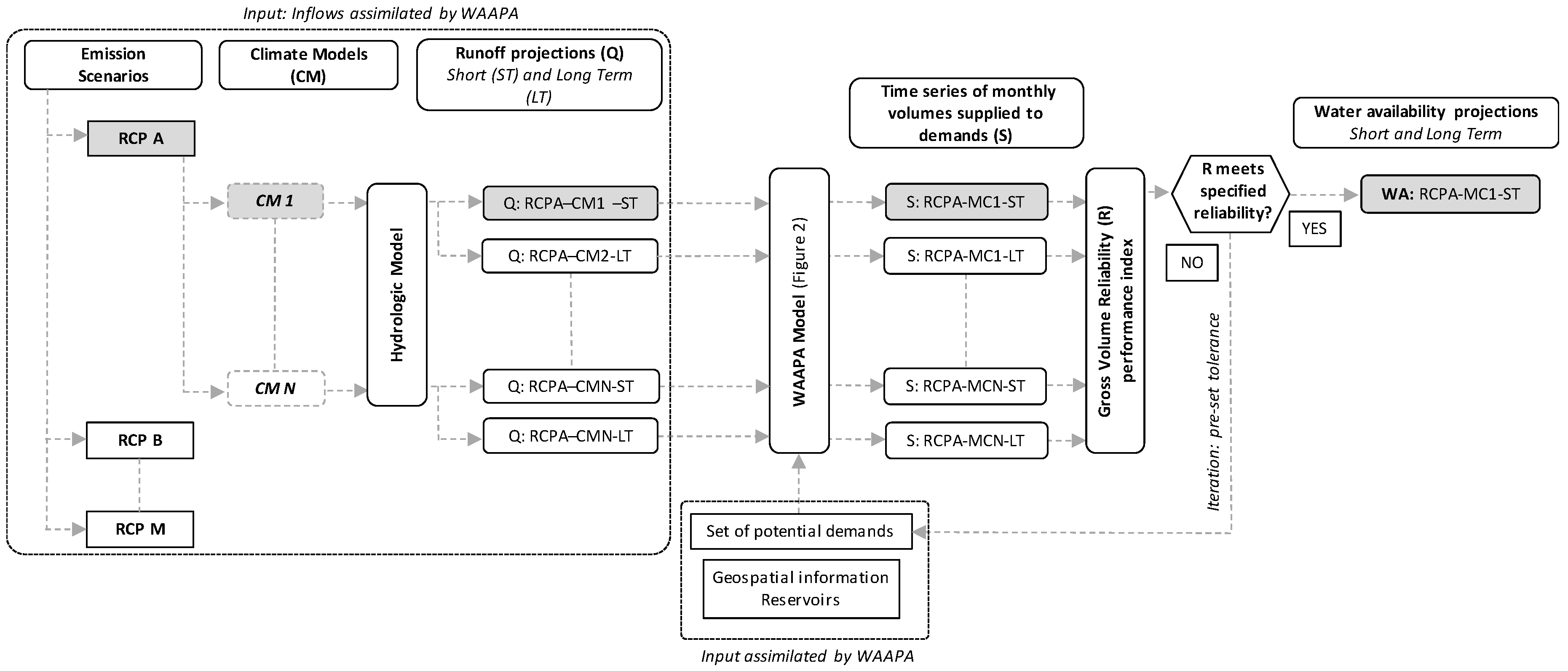
The methodological approach is detailed in Figure 1. The methodology is based on a high-resolution GIS-based model, named “Water Availability and Adaptation Policy Assessment (WAAPA)” which enables the estimation of water availability under many climate scenarios to produce a global picture of the situation [33]. The model assimilates climate and geospatial information seamlessly, accounts for reservoir storage (from an individual reservoir or from a system of reservoirs), and produces blue water availability estimates. The model computes net blue water availability for consumptive use of a river basin, taking into account the regulation capacity of its water supply system, and a set of management standards defined by water policy. The model estimates the water availability not only at the outlet of sub-basins (e.g., river intersections), but also at any desired point of the defined river network (e.g., each dam location), by accounting for the entire system of dams in the upstream basin. Basic components of WAAPA are reservoirs, inflows, and demands and they are linked to nodes of the river network. The joint reservoir operation model simulates the behaviour of a set of reservoirs that supply water for a set of prioritized demands, complying with specified ecological flows and accounting for evaporation losses.
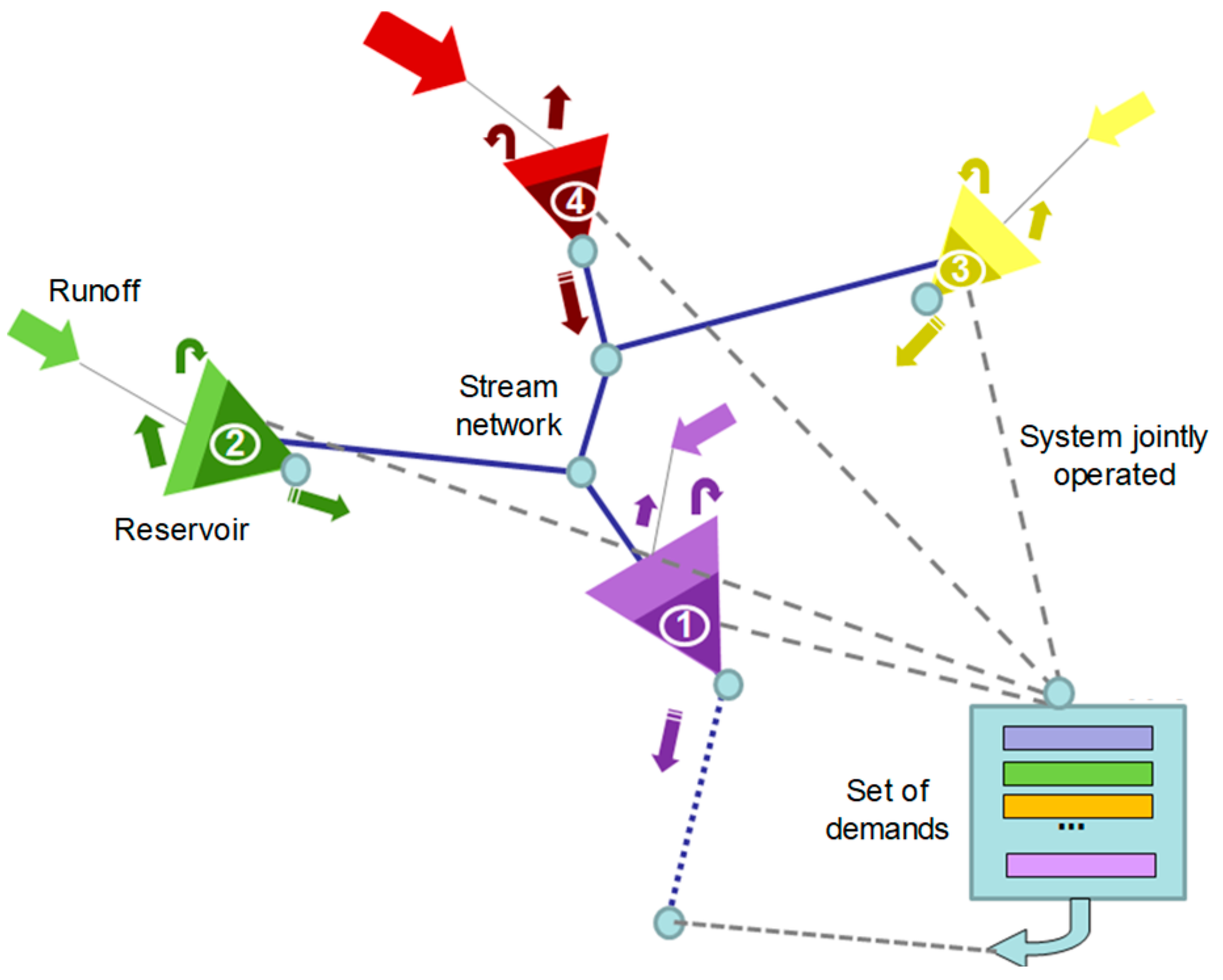
In this study, we evaluated the water availability of the joint reservoir operation model following a high resolution and global management scheme (Figure 2). For each selected sub-basin (derived from dam locations and river confluences), this scheme considers each reservoir individually and all reservoirs are jointly operated to supply a set of prioritized demands. It is assumed that any demand at a given point in the stream network can be supplied by any reservoir located upstream from it. It corresponds to a situation where there is little development of system interconnections, but a large development of water distribution networks, which are managed globally to supply all demands present in the analysed system. Water is first released (to satisfy demands) from the reservoirs located at low areas of the basin. If these reservoirs are full and receive more contributions, uncontrolled spills are released and water falls out of the system. On the other hand, if upstream reservoirs are full and receive more inflows, the extra water is collected by the downstream reservoirs. This management criterion is not totally real, because real systems usually are managed taking into account more conditions and constraints. The joint reservoir operation model maximizes water availability because it minimizes the excess storage. In each time step, the model performs the following operations:
- It satisfies the environmental flow requirement in every reservoir with the available inflow. Environmental flows are passed to downstream reservoirs and added to their inflows.
- It computes evaporation in every reservoir and reduces storage accordingly.
- It computes excess storage (storage above maximum capacity) in every reservoir (if there is an increment of storage with the remaining inflow).
- It satisfies demands ordered by priority, if possible. It uses excess storage first, then available storage starting from higher priority reservoirs.
- If excess storage remains in any reservoir, it computes uncontrolled spills.
The result of the joint reservoir operation model is a set of time series of monthly volumes supplied to each demand, monthly storage values, monthly values of spills, environmental flows, and evaporation losses in every reservoir. Finally, we calculated the system performance by applying the Gross Volume Reliability performance index. This index is the ratio of total volume supplied to demand in the system and the total volume demanded by the system, during the analysed period [33]. In this study, water availability is estimated by considering only one demand present in the system under the hypothesis of 90% reliability.
To define the maximum amount of water that can be supplied at a certain point of the river network to satisfy a regular demand, a bipartition method is applied: Excessive values of demands are set (for example, similar to mean monthly runoff) and the simulation is carried out. The deficits are obtained and specified reliability requirements are checked. If the specified reliability requirements are not fulfilled, the demand is reduced by half and simulated again. If the specified reliability requirements are satisfied, half of the difference is added and simulated again, and so on until the deficit (or gain) is smaller than a pre-set tolerance (e.g., 0.1 hm3/year).
Case Study
The area under analysis is composed of the major river basins in Western Europe. WAAPA model data are geographically referenced (Figure 3). Following, we present the data used to build the WAAPA model. We determined the topology of the model by dividing the area under study into a number of units of analysis, which are homogeneous sub-basins from the water management perspective. The sub-basins are related through the “drain to” relationship, and the analysis is applied to all possible basins, from the small headwater sub-basins to the largest basin draining to the sea. In this work, we divided western Europe into sub-basins (3839), based on the Hydro1k data set (1.538 sub-basins [41]), and the derived-from dam locations (2.301 sub-basins), which belong to 621 large basins draining to the sea. The total area under study is over 6,000,000 km2.
Naturalized streamflow was obtained from the results of the application of the PCRGLOBWB model [42] to the Inter-Sectoral Impact Model Inter-Comparison Project [43]. The PCRGLOBWB model was run for the entire globe at 0.5° resolution, using forcing from five global climate models under historical conditions and climate change projections, corresponding to four Representative Concentration Pathways scenarios: RCP2.6, RCP4.5, RCP6.0, and RCP8.5. The following climate models were used as input: GFDL-ESM2NM (GFDL), HadGEM2-ES (HadGEM2), IPSL-CM5A-LR (IPSL), MIROC-ESM-CHEM (MIROC), and NorESM1-M (NorESM1).
Three time periods were considered: Reference (1960–1999), short term (ST, 2020–2059), and long term (LT, 2060–2099). Since runoff obtained from climate model input usually presents significant bias, average runoff values were corrected for bias using the UNH/GRDC (University of New Hampshire/Global Runoff Data Centre) composite runoff field, which combines observed river discharges with a water balance model [44], and is a reference of the current global surface runoff [34,44,45]. Following González-Zeas [45], we applied the bias-correction methodology based on the determination of a monthly correction factor. We calculated the monthly mean runoff series for the control scenario to obtain twelve representative statistical parameters: The ratios between the UNH/GRDC values (observed) and the simulated runoff. These multiplying factors were used to correct bias in the control and the projected series. The reservoir storage volume available for regulation in every sub-basin was obtained from the ICOLD World Register of Dams [46]. Dams in the register with more than 5 hm3 of storage capacity were georeferenced and linked to the corresponding storage capacity and flooded area (2.301 dams). Environmental flows were computed through a hydrologic method. The minimum environmental flow was set to the 10% percentile of the marginal monthly distribution, according to Spanish legislation. In the absence of more advanced methods, the Spanish regulation for river basin plans establishes several hydrologic methods to define minimum environmental flows [31]. One of them is based on the percentile of the marginal distribution of monthly flows, defining a range between 5 and 15%.
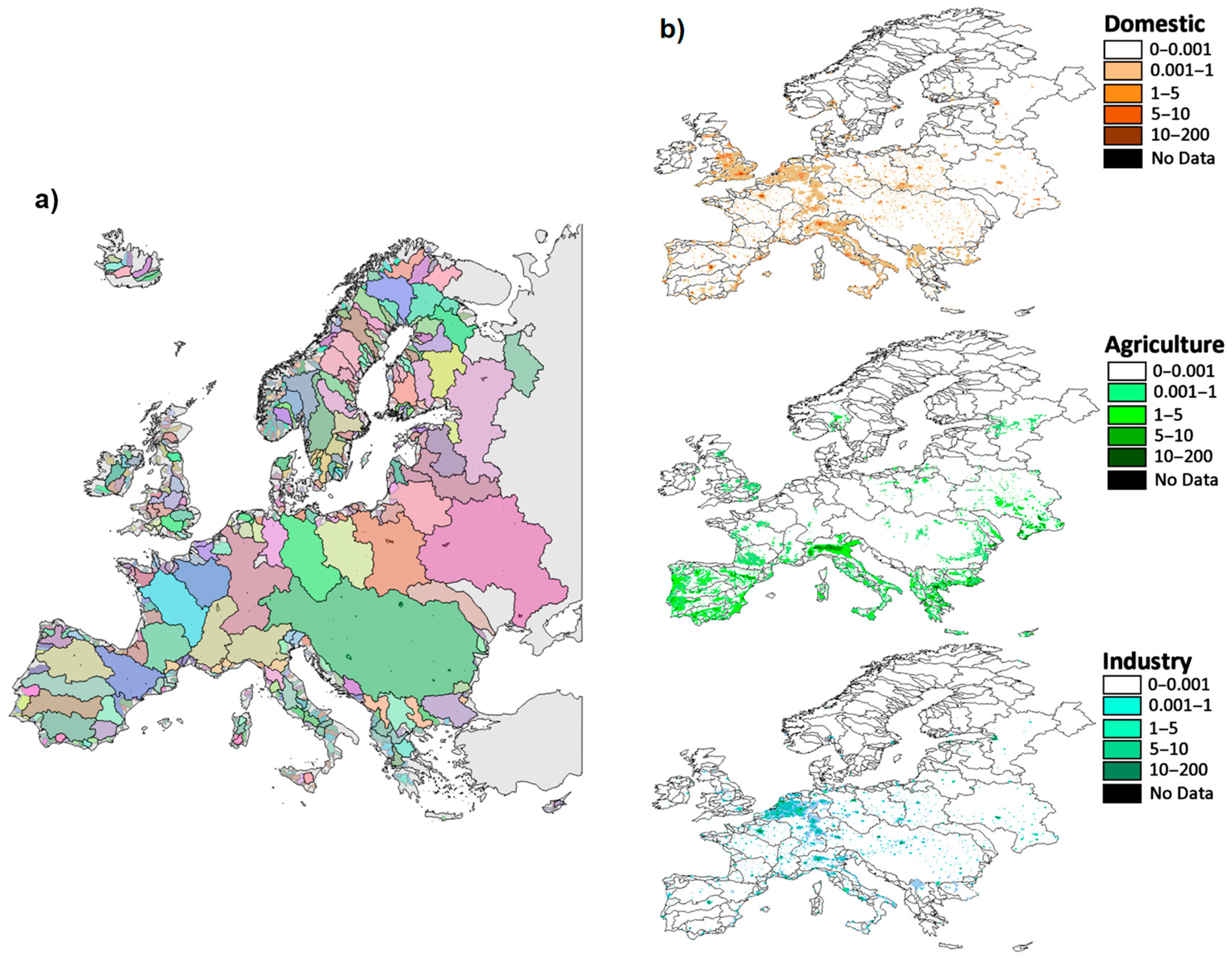
In this study, we estimated current, short-, and long-term geographically distributed water withdrawals. Country-based data on current freshwater withdrawal were taken from the World Bank database. These data were spatially distributed using proxy variables: Population density for urban and industrial withdrawals and irrigated area for agricultural withdrawals. The population density was obtained from the Gridded Population of the World product of the Global Rural–Urban Mapping Project (GRUMP), available at the Centre for International Earth Science Information Network (Figure 3b) [47]. The area potentially under irrigation was estimated from the Global Map of Irrigated Area dataset [48]. Future withdrawals were estimated using the projections of population and gross domestic product (GDP) provided by IIASA. These projections were estimated following RCP scenario assumptions [38,39]. Projections of total freshwater withdrawal and industrial withdrawal were estimated from regressions based on World Bank data using per capita GDP projections [40].
3. Results
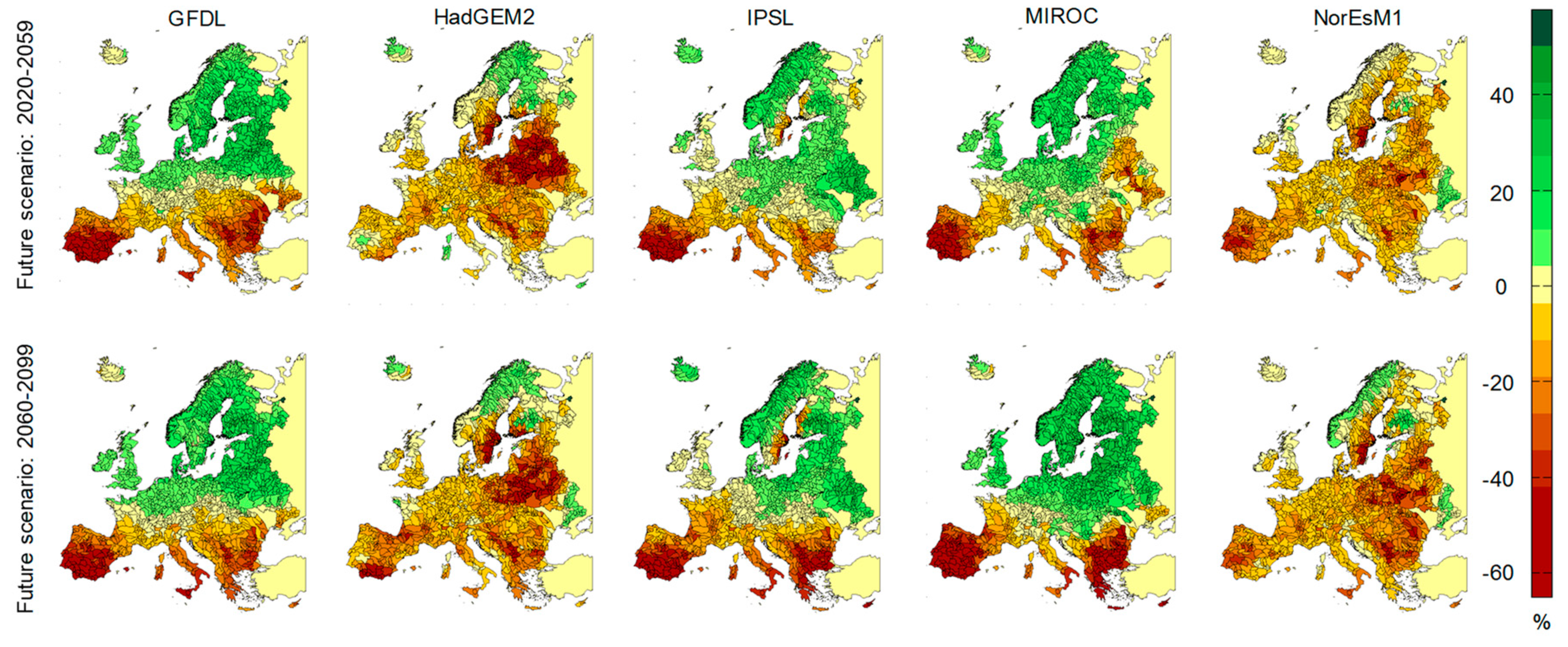
Figure 4 shows the comparison of streamflow change from reference (1960–1999) to climate change RCP4.5 scenarios, both for short (2020–2059) and long term (2060–2099), and over the five climate models. Figure 4 is dimensionless (percentage), and the values were obtained by applying Equation (1). The red shading represents a decrease (negative values) and green shading an increase (positive values) of the future mean annual runoff. The yellow shading represents no changes of mean annual runoff for future periods compared to the reference scenario.
Overall, the models produce a smooth picture of mean annual runoff change in Europe, with decreases in the South. Severe negative changes are projected in the Iberian Peninsula, from the Black Sea in the South almost to the Baltic Sea in the North, and predominantly positive changes are projected in western to central Europe and in northern Europe. A mixed pattern with higher variability in mean annual runoff is shown across central Europe and the Carpathians. The climate models that produce more annual runoff reduction are HadGEM2 and NorEsM1. However, it can be seen that the values and spatial extent of the regions with reduced streamflow (in brownish colours) vary significantly from one climate model to another. This is remarkable considering that all simulations were performed with the same hydrologic model. As expected, in general, the changes are more intense in the long-term period. The region of neutral changes (represented in yellow) moves toward the north from low carbon (RCP2.6) to high carbon (RCP8.5) emissions scenarios (not shown).
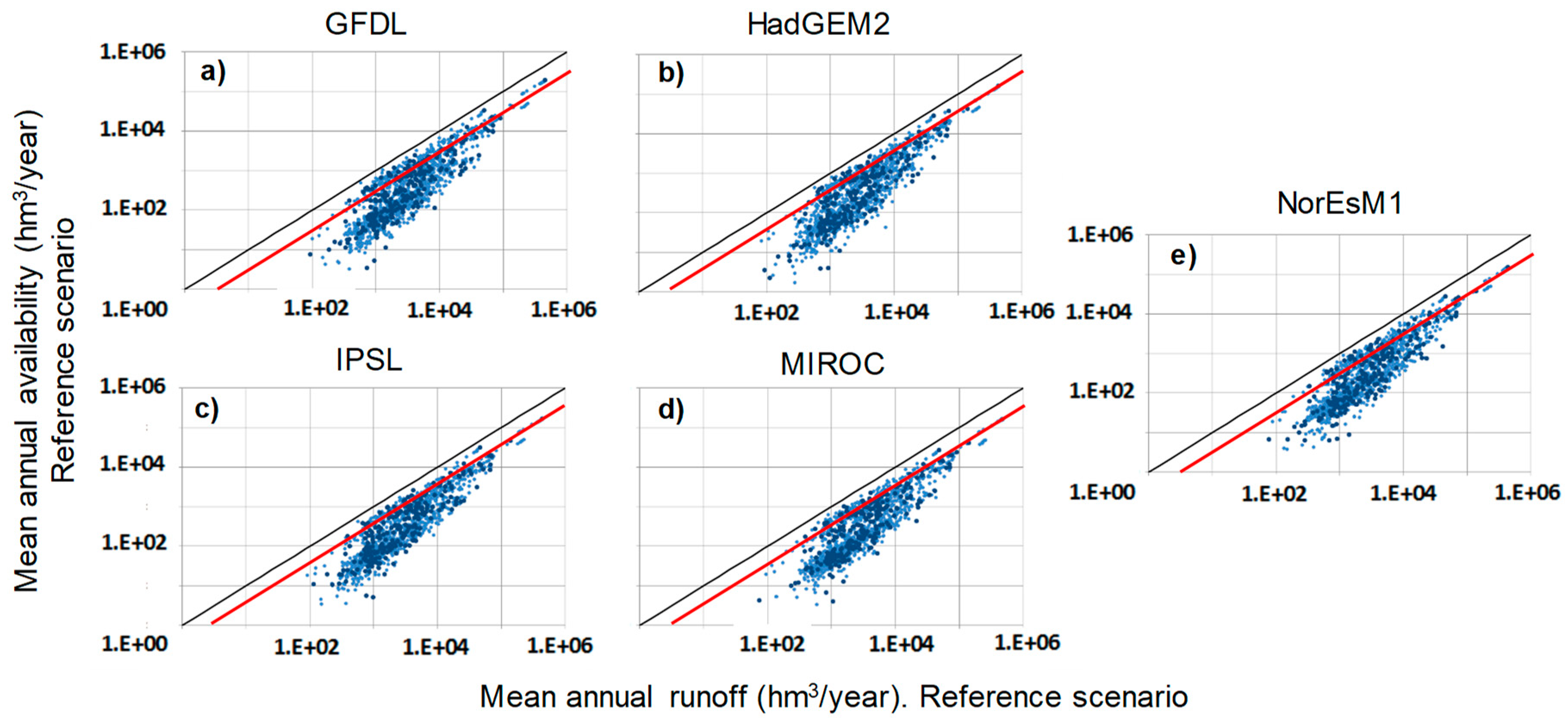
The results of potential water availability in historical conditions (1960–1999) for all climate models are shown in Figure 5. It shows the values of potential water availability as a function of mean annual runoff in all the analysed sub-basins. Small, blue dots represent results in intermediate sub-basins, while larger, darker blue dots represent results in the global basins. All models show a similar picture, with a large variation of water availability among basins as a consequence of differences in hydrologic regime and reservoir storage.
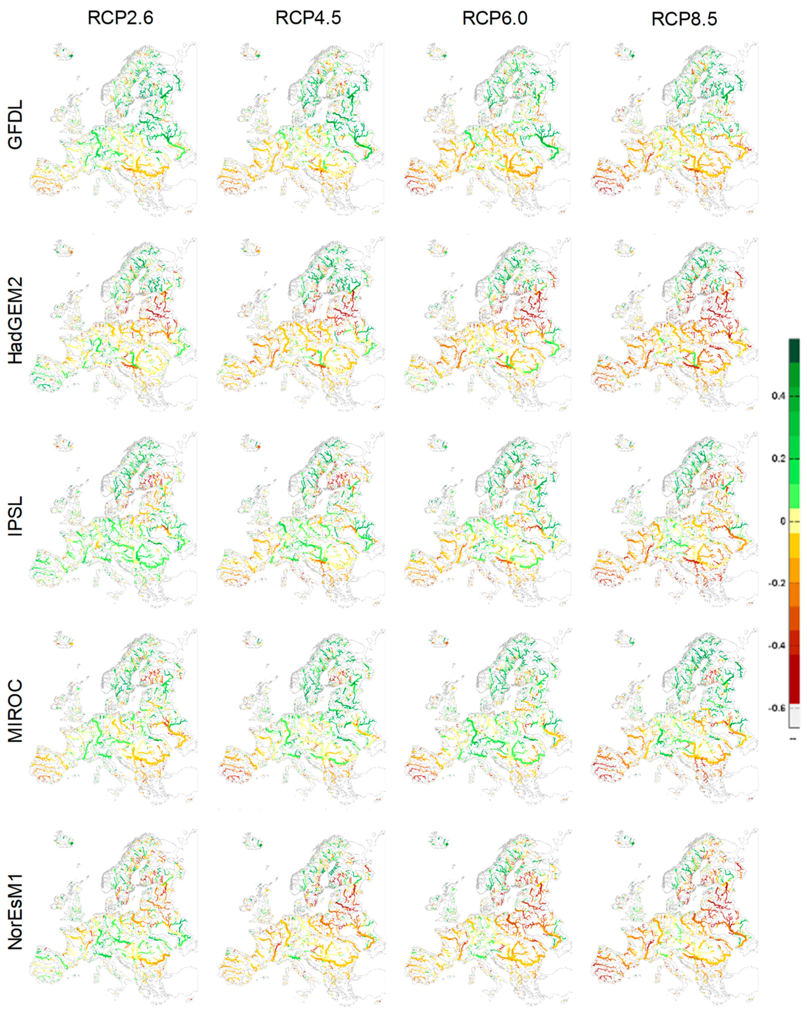
The spatial distribution of changes (between the long term and reference periods) of potential water availability along the major rivers in Europe is presented in Figure 6, for all emissions scenarios and climate models analysed. Figure 6 is dimensionless, and the values were obtained by applying an equation similar to Equation 1, but using potential water availability instead of runoff. Red shading represents a decrease (negative values) of the future potential water availability and green shading an increase (positive values). The yellow shading represents no changes of potential water availability compared to the reference scenario. Although, in general, the climate models show a gradient of potential water availability changes with larger reductions in South Western Europe and larger increases in Northern Europe, values show important differences by comparing the results among climate models (same emissions scenario). By comparing the maps within each column (Figure 6), we visualize important differences in the results from one climate model to another, and by keeping each emissions scenario unaltered. The models that produce the most potential water availability reduction are HadGEM2 and NorEsM1, while IPSL and MIROC produce the least reductions. On the other hand, by comparing the maps within each row (Figure 6), we observe the different results obtained for the same climate model and different emissions scenarios. It can be seen that, in general, differences among the emissions scenarios (for each climate model) are smaller than those among different models (for each emissions scenario). The driest scenario is RCP8.5 for all analysed climate models.
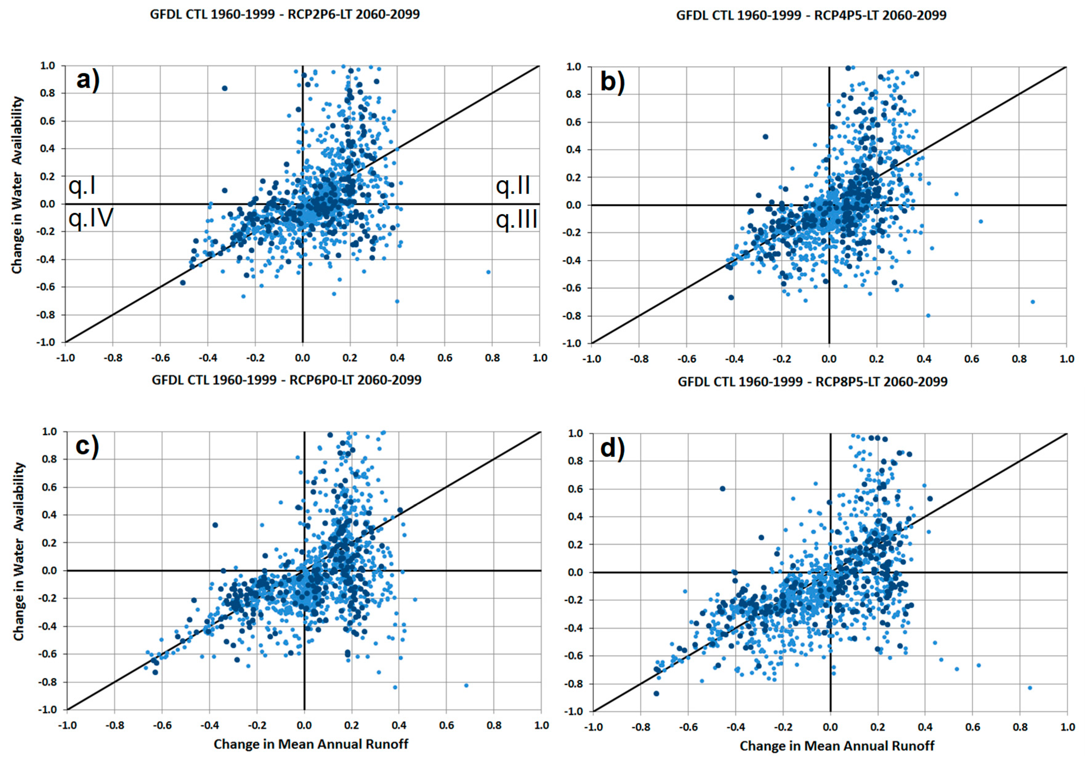
Figure 7 shows, for each analysed sub-basin, the changes in the potential water availability in the long-term period with respect to the reference period (y axis), as a function of changes in the mean annual runoff in the long-term period with respect to the reference period (x axis), for all emissions scenarios and the climate model GFDL. The equations used to plot the results are similar to the proposed Equation 1 for the runoff variable (see Figure 4) and the proposed for the water availability variable (see Figure 6). Quadrant 1 (q.I) shows sub-basins where runoff decreases in the future and water availability increases. Both runoff and water availability increase in q.II, runoff increases and water availability decreases in q.III, and both runoff and water availability decrease in q.IV. In addition, basins with the same reduction of runoff experience different reductions in availability as a result of changes in the hydrologic variability and their different regulation capacity.
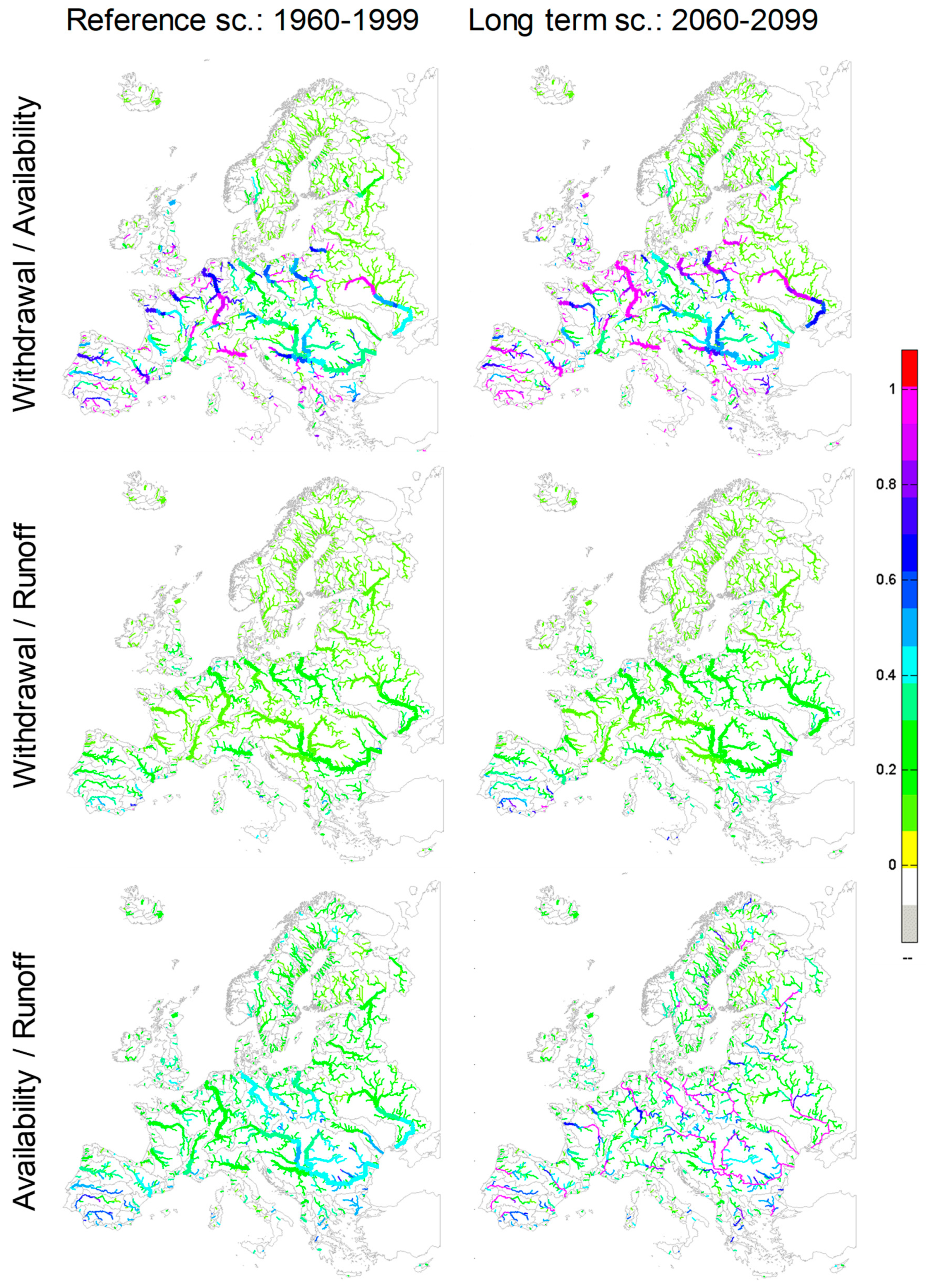
Figure 8 shows the spatial distribution of the ratio of the runoff, water availability, and water withdrawal for the model GFDL in emissions scenario RCP4.5 for the reference (1960–1999) and long-term period (2060–2099). The bottom row shows potential water availability as a fraction of runoff, the central one shows water withdrawal, also as a fraction of runoff, and the upper row shows the water withdrawal as a fraction of water availability.
Figure 9 shows the uncertainty associated with the climate models and emissions scenarios, both for mean annual runoff and mean water availability, by calculating the coefficient of variation (CV, standard deviation divided by mean) in each calculation point, for each climate model (five), for each emissions scenario (four) and for the short term (ST) and the long term (LT). We represented the probability distribution function (Pdf) of the CVs in each case. Continuous lines represent the uncertainty for each climate model, obtained by comparing the four emissions scenarios for each climate model. The dashed lines represent uncertainty for each emissions scenario, obtained by comparing the CV of the five models for each emissions scenario. Figure 9a,c shows the uncertainty associated with runoff for the ST and LT, respectively. Comparatively, Figure 9b,d shows the uncertainty associated with availability for the ST and LT, respectively.
4. Discussion
Both for short- and long-term periods, the models show similar spatial patterns of mean annual runoff changes in Europe, with decreases in the south, especially in the south-west and increases in the north. Our results agree with global and continental-scale studies that reported mean annual runoff projections [1,49,50]. These studies provide a coherent pattern of change in annual runoff, predicting with a high degree of confidence severe decreases (up to 40%) of surface runoff in areas already affected by water scarcity, like the Mediterranean region, and are consistent with the projected runoff increases in northern Europe (5–30%). However, it can be seen that the values and spatial extent of the regions with reduced streamflow vary significantly from one climate model to another. It suggests that there is an important climate model uncertainty, being the changes of mean annual runoff among emissions scenarios (and the same climate model) smaller than those among the different climate models (same emissions scenario).
In the short-term runoff, Figure 9a clearly shows that higher CV values are more frequent (amplitude of each Pdf curve) by comparing the results among models (and the same emissions scenario, dashed lines) than among emissions scenarios (and the same climate model, continuous lines). In addition, the uncertainties associated with the emissions scenarios are also similar among them (differences among continuous lines for the y axis). Although climate change models are the most robust tools available to generate consistent climate change projections, they are still a source of considerable uncertainties [10,51]. In this regard, Garrote [18] highlighted that the uncertainty has not been reduced with the progressive improvement of modelling tools; on the contrary, it seems to be increasing as a result of the evolving approach to generating emissions scenarios. On the other hand, results suggest that, because of the number of variables and complexity involved in the estimation of the future climate, its estimation has an implicit uncertainty that should be acknowledged for the development of climate adaptation plans. In the long-term runoff (Figure 9c), the uncertainty increases (increasing the amplitude of the Pdf curves) for both climate models and emissions scenarios, although climate models remain more uncertain than emissions scenarios. Also, greater dispersion of uncertainty is found among models than among emissions scenarios. It could be partially explained by the increase of the differences between emissions scenarios for the long-term analysis. These results are consistent with several inter-comparison studies that also show considerable variability in the magnitude and timing of the projected runoff [9,49,50,52,53]. At this point, it is remarkable that all simulations in this study were performed with the same hydrologic model. Databases of climate scenarios are available from different research projects [54,55], including surface runoff among their output variables. As the characterization of the water cycle in the models used in these types of studies usually is very simple and results provide a low signal-to-noise ratio (especially in arid and semi-arid regions), varying the large-scale hydrological models incorporates an additional source of uncertainty [18,50,52]. Some authors state that hydrologic model uncertainties are less significant than those originating from climate change models [9,56].
Changes in potential water availability in short- and long-term scenarios according to all climate models and emissions scenarios were analysed. High resolution results showed similar future spatial patterns to mean annual runoff, with the differences among the emissions scenarios (for each climate model) being smaller than those among different models (for each emissions scenario). Figure 9b shows that the uncertainty associated with the emissions scenarios increases and their values draw near to the climate model uncertainties. Furthermore, the Pdfs of the uncertainty associated with the climate models for water availability remain similar to that for runoff. Similar behaviour is observed for the long-term period (Figure 9d). It suggests that the management of hydraulic infrastructures (mainly reservoirs in this study) plays an important role by decoupling water availability from hydrologic variability. This is observed for all climate models and emissions scenarios considered. Svensson et al. [57] reinforced the importance of the installation of reservoirs in several river basins in Europe in the last century, by attenuating the basins’ drought conditions. For quantifying and summarizing purposes, Table 1 shows the emissions scenarios’ and climate models’ uncertainty for the 50% probability of exceeding CV values. Several local and regional studies agree that the propagation of the uncertainties affects water resource system performances [26,58,59,60]. Thus, the assessment (or projection) of the performance of a water resources system should be evaluated with extreme care. As previously stated, the reservoir operation model applied in WAAPA is highly simplified and was designed to maximize water availability. Thus, the reality of reservoir operation is much more complex. Usually, not all reservoirs in the basin are jointly managed to supply all demands. They are either managed individually to supply local demands or grouped in systems that are managed independently. Availability of storage volume for water conservation management is also variable according to local conditions, due to the need to allocate storage volume to flood control. Therefore, it is unlikely that upstream reservoirs are kept full to release space in downstream reservoirs. Normal operation would tend to balance storage in all reservoirs to prevent uncontrolled spills. In practice, the spatial pattern of water availability will differ from that obtained in WAAPA. WAAPA results should only be considered as an upper bound of the actual water availability that could be obtained in practice.
Results from the comparisons of the changes in potential water availability with changes in runoff clearly show how changes in the former are not proportional to changes in the latter, suggesting the inadequacy of methodologies that estimate availability as a fraction of mean annual runoff. As an example, in Figure 5, the red line shows the traditional value of 40% of the mean annual runoff adopted for water availability when no simulation of reservoir regulation is performed [61]. It can be seen that adopting this constant value as a proxy of water availability can be strongly misleading, since only those basins with very regular flow or very large reservoir storage can reach this value. In most basins, water availability is a smaller fraction of the mean annual runoff.
As shown, availability and withdrawal are only a small fraction of runoff in most of Europe and their projected changes are small, except for the south-east and the south-west. However, the representation of the water withdrawal as a fraction of water availability (Figure 8, upper row) shows that these two variables have similar values in many regions of Europe, and that they are getting closer in the long-term scenario. It means that in many regions, water shortage struggles to satisfy the demand with a specific reliability could emerge or increase, both for the present and future periods. It can also be seen that the relationship between these variables is complex, and that it varies significantly among regions, depending on hydrologic regime, climate, reservoir storage, and socioeconomic factors.
Green water (not analysed in this study), similarly to blue water, is also expected to decrease in most of western Europe except for northern countries. However, changes in green water result from complex interplay of impacts on precipitation, temperature, and CO2 concentration, which ultimately affects potential evapotranspiration, soil moisture conditions, and growing periods. Thus, patterns of expected changes differ for green and blue water [62]. Irrigation demands will also be affected, due to modified seasonal patterns and evapotranspiration demands [36,63].
Finally, some limitations of this study should be noted. We estimated the potential water availability (upper theory limit) by considering only one demand present in the system. System performance was evaluated as gross volume reliability. Potential water availability was obtained under the hypothesis of 90% reliability. The data used in this study were obtained from specific climate models and emissions scenarios, thus, the conclusions derived from this study are inextricably affected by the models’ uncertainty. Additionally, we made a series of simplifying assumptions. We assumed variable geographic and temporal water withdrawals, both in the present and future climate, from indirect methods (GDP and population). We assumed that the reservoirs, whose sole purpose was hydropower generation, were not included in the systems to manage the water resources. We considered that the hydraulic infrastructure corresponding to each analysed sub-basin (determined from a given point in the stream network) was being jointly managed to supply global demands, while in some real cases it could have been divided in to several rather independent subsystems. Furthermore, in our model, there were no system interconnections nor a large-scale water distribution infrastructure. We did not consider other sources of uncertainty as, for instance, the observed climate data source or the hydrologic model applied and the inclusion of regional climate models (RCMs). It is expected that RCMs have less associated uncertainty than GCMs when a particular region is analysed, as they account for more detailed and specific regional characteristics.
5. Conclusions
This study presents the potential water availability changes under alternative climate change scenarios in western Europe. Results are geographically referenced at high resolution across the major European river basins. The study includes the estimation of the associated uncertainties, resulting from differences among climate change scenarios and climate models. The authors are not aware of similar studies conducted at such a high-resolution continental scale. In this study, we applied the WAAPA model on a high-resolution dataset to analyse water availability changes across western Europe. The proposed model and the applied methodology demonstrated their ability to perform regional studies covering extensive domains, while maintaining high resolution on the characterization of the systems. The climate models that produced the most reduction of mean annual runoff and potential water availability were HadGEM2 and NorEsM1, while IPSL and MIROC produced the least reduction. Overall, for both mean annual runoff and potential water availability, a gradually varying picture of change in Europe was observed, with a decrease in the south (especially in the south-west) and an increase in the north. Moreover, the region of neutral changes moves to the north, from low carbon (RCP2.6) to high carbon (RCP8.5) emissions scenarios. Climate model uncertainties for mean annual runoff and potential water availability were found to be higher than scenario uncertainties. This conclusion was derived by comparing the variability of the results obtained, while the PCRGLOBWB model was forced with different climate models under the same emissions scenario to that of the results from different emissions scenarios for the same climate model forcing. Thus, although climate change models are the most robust tools available to generate consistent climate change projections, they are still a source of considerable uncertainties and their results should be carefully used for operative purposes.
While potential water availability and water withdrawal are only a small fraction of runoff in most of Europe for current and future scenarios (except in the south-east and the south-west of Europe), water withdrawal and water availability are similar in many regions of Europe, and they are getting closer in the long-term scenario (2060–2099). Thus, the balance between water availability and withdrawals is threatened in some regions. Furthermore, social factors, like management of hydraulic infrastructure, play an important role by decoupling water availability from hydrologic variability. This is observed for all climate models and emissions scenarios considered. Finally, although this study presents significant progress in terms of spatial scale and detail compared to previous studies, it is still only indicative of the importance of regional change, due to the assumptions and uncertainties discussed. Nevertheless, the results are useful for envisioning potential water resource system conflicts and contributing to the identification of regions where an in-depth analysis may be necessary.
Supplementary Materials
The following are available online at https://www.mdpi.com/2073-4441/11/3/420/s1.
Author Contributions
Conceptualization, L.G. and A.I.; methodology, A.S.-W. and A.I.; software, L.G.; investigation and formal analysis, A.S.-W. and I.G.; resources and data curation, I.G.; writing—original draft preparation, I.G.; writing—review and editing, A.S.-W.; visualization and supervision, L.G.; funding acquisition, A.S.-W. and A.I.
Funding
This research was partially funded by Universidad Politécnica de Madrid through the “Programa propio: ayudas a proyectos de I+D de investigadores posdoctorales” and the “ADAPTA” project. We also acknowledge the financial support of the European Commission BASE project (grant agreement no.: ENV-308337) of the 7th Framework Program (http://base-adaptation.eu).
Conflicts of Interest
The authors declare no conflict of interest.
References
- IPCC 2014. Climate Change 2014: Impacts, Adaptation, and Vulnerability Part A: Global and Sectoral Aspects; Contribution of Working Group II to the Fifth Assessment Report of the Intergovernmental Panel on Climate Change 2014; Field, C.B., Barros, V.R., Dokken, D.J., Mach, K.J., Mastrandrea, M.D., Bilir, T.E., Chatterjee, M., Ebi, K.L., Estrada, Y.O., Genova, R.C., et al., Eds.; Cambridge University Press: Cambridge, UK; New York, NY, USA, 2017; pp. 1–32. [Google Scholar]
- European Environment Agency (EEA). Climate Change, Impacts and Vulnerability in Europe 2016. An Indicator-Based Report; EEA Report No 1/2017; European Environment Agency: Copenhagen, Denmark, 2017. [Google Scholar]
- Arnell, N.W.; Van Vuuren, D.P.; Isaac, M. The implications of climate policy for the impacts of climate change on global water resources. Glob. Environ. Chang. 2011, 21, 592. [Google Scholar] [CrossRef]
- Alcamo, J.; Floerke, M.; Maerker, M. Future long-term changes in global water resources driven by socioeconomic and climatic changes. Hydrol. Sci. 2007, 52, 247–275. [Google Scholar] [CrossRef]
- Easterling, D.R.; Meehl, J.; Parmesan, C.; Changnon, S.A.; Karl, T.R.; Mearns, L.O. Climate extremes: Observations, modeling, and impacts. Science 2000, 289, 2068–2074. [Google Scholar] [CrossRef] [PubMed]
- Vörösmarty, C.J.; McIntyre, P.B.; Gessner, M.O.; Dudgeon, D.; Prusevich, A.; Green, P.; Glidden, S.; Bunn, S.E.; Sullivan, C.A.; Liermann, C.R.; et al. Global threats to human water security and river biodiversity. Nature 2010, 467, 555. [Google Scholar] [CrossRef] [PubMed]
- Chawla, I.; Mujumdar, P.P. Partitioning uncertainty in streamflow projections under nonstationary model conditions. Adv. Water Resour. 2108, 112, 266–282. [Google Scholar] [CrossRef]
- Yen, H.; Wang, X.; Fontane, D.G.; Harmel, R.D.; Arabi, M. A framework for propagation of uncertainty contributed by parameterization, input data, model structure, and calibration/validation data in watershed modeling. Environ. Model. Softw. 2014, 54, 211–221. [Google Scholar] [CrossRef]
- Gao, J.; Sheshukovb, A.Y.; Yena, H.; Douglas-Mankin, K.R.; White, M.J.; Arnold, J.G. Uncertainty of hydrologic processes caused by bias-corrected CMIP5 climate change projections with alternative historical data sources. J. Hydrol. 2019, 568, 551–561. [Google Scholar] [CrossRef]
- Déqué, M.; Somot, S.; Sanchez-Gomez, E.; Goodess, C.M.; Jacob, D.; Lenderink, G.; Christensen, O.B. The spread amongst ENSEMBLES regional scenarios: Regional climate models, driving general circulation models and interannual variability. Clim. Dyn. 2012, 38, 951–964. [Google Scholar] [CrossRef]
- Falkenmark, M.; Rockström, J. The New Blue and Green Water Paradigm: Breaking New Ground for Water Resources Planning and Management. Water Resour. Plan. Manag. 2006, 132, 129–132. [Google Scholar] [CrossRef]
- García-Ruiz, J.M.; López-Moreno, J.I.; Vicente-Serrano, S.M.; Lasanta–Martínez, T.; Beguería, S. Mediterranean water resources in a global change scenario. Earth Sci. Rev. 2011, 105, 121–139. [Google Scholar] [CrossRef] [Green Version]
- Gardner, L.R. Assessing the effect of climate change on mean annual runoff. J. Hydrol. 2009, 379, 351–359. [Google Scholar] [CrossRef]
- Simonovic, S.P. Managing Water Resources: Methods and Tools for a Systems Approach; UNESCO Publishing: Paris, France, 2009. [Google Scholar]
- Nilsson, C.; Reidy, C.A.; Dynesius, M.; Revenga, C. Fragmentation and flow regulation of the World’s large river systems. Science 2005, 308, 405–408. [Google Scholar] [CrossRef] [PubMed]
- Iglesias, A.; Santillán, D.; Garrote, L. On the Barriers to Adaption to Less Water under Climate Change: Policy Choices in Mediterranean Countries. Water Resour. Manag. 2018. [Google Scholar] [CrossRef]
- Iglesias, A.; Garrote, L. Adaptation strategies for agricultural water management under climate change in Europe. Agric. Water Manag. 2015, 155, 113–124. [Google Scholar] [CrossRef] [Green Version]
- Garrote, L. Managing Water Resources to Adapt to Climate Change: Facing Uncertainty and Scarcity in a Changing Context. Water Resour. Manag. 2017, 31, 2951–2963. [Google Scholar] [CrossRef]
- Vogel, R.M.; Sieber, J.; Archfield, S.A.; Smith, M.P.; Apse, C.D.; Huber-Lee, A. Relations among storage, yield, and instream flow. Water Resour. Res. 2007, 43, W05403. [Google Scholar] [CrossRef]
- Arnold, J.; Bieger, K.; White, M.; Srinivasan, R.; Dunbar, J.; Allen, P. Use of Decision Tables to Simulate Management in SWAT+. Water 2018, 10, 713. [Google Scholar] [CrossRef]
- White, M.J.; Gambone, M.; Yen, H.; Arnold, J.; Harmel, D.; Santhi, C.; Haney, R. Regional Blue and Green Water Balances and Use by Selected Crops in the U.S. J. Am. Water Resour. Assoc. 2015, 51, 1626–1642. [Google Scholar] [CrossRef]
- Wurbs, R.A.; Muttiah, R.S.; Felden, F. Incorporation of climate change in water availability modeling. J. Hydrol. Eng. 2005, 10, 375. [Google Scholar] [CrossRef]
- Yates, D.; Sieber, J.; Purkey, D.; Huber-Lee, A. WEAP21—A demand-, priority-, and preference-driven water planning model. Part 1: Model characteristics. Water Int. 2005, 30, 487–500. [Google Scholar] [CrossRef]
- Andreu, J.; Capilla, J.; Sanchís, E. AQUATOOL, a generalized decision-support system for water-resources planning and operational management. J. Hydrol. 1996, 177, 269–291. [Google Scholar] [CrossRef]
- Harou, J.J.; Pulido-Velazquez, M.; Rosenberg, D.E.; Medellín-Azuara, J.; Lund, J.R.; Howitt, R.E. Hydro-economic models: Concepts, design, applications, and future prospects. J. Hydrol. 2009, 375, 627–643. [Google Scholar] [CrossRef] [Green Version]
- Sordo-Ward, A.; Granados, I.; Martín-Carrasco, F.; Garrote, L. Impact of Hydrological Uncertainty on Water Management Decisions. Water Resour. Manag. 2016, 30, 5535–5551. [Google Scholar] [CrossRef]
- Chávez-Jimenez, A.; Lama, B.; Garrote, L.; Martin-Carrasco, F.; Sordo-Ward, A.; Mediero, L. Characterisation of the Sensitivity of Water Resources Systems to Climate Change. Water Resour. Manag. 2013, 27, 4237–4258. [Google Scholar] [CrossRef]
- World Water Assessment Programme (WWAP). The United Nations World Water Development Report 4: Managing Water under Uncertainty and Risk; UNESCO: Paris, France, 2012. [Google Scholar]
- Moss, R.H.; Edmonds, J.A.; Hibbard, K.A.; Manning, M.R.; Rose, S.K.; Van Vuuren, D.P.; Carter, T.R.; Emori, S.; Kainuma, M.; Kram, T.; et al. The next generation of scenarios for climate change research and assessment. Nature 2010, 463, 747–756. [Google Scholar] [CrossRef] [PubMed]
- Estrela, T.; Perez-Martin, M.A.; Vargas, E. Impacts of climate change on water resources in Spain. Hydrol. Sci. J. 2012, 57, 1154–1167. [Google Scholar] [CrossRef] [Green Version]
- Pulido-Velazquez, D.; Garrote, L.; Andreu, J.; Martin-Carrasco, F.J.; Iglesias, A. A methodology to diagnose the effect of climate change and to identify adaptive strategies to reduce its impacts in conjunctive-use systems at basin scale. J. Hydrol. 2011, 405, 110–122. [Google Scholar] [CrossRef] [Green Version]
- Iglesias, A.; Garrote, L.; Diz, A.; Schlickenrieder, J.; Martin-Carrasco, F. Rethinking water policy priorities in the Mediterranean region in view of climate change. Environ. Sci. Policy 2011, 14, 744–757. [Google Scholar] [CrossRef]
- Garrote, L.; Iglesias, A.; Granados, A.; Mediero, L.; Martin-Carrasco, F. Quantitative assessment of climate change vulnerability of irrigation demands in Mediterranean Europe. Water Resour. Manag. 2015, 29, 325–338. [Google Scholar] [CrossRef]
- Abbaspoura, K.C.; Rouholahnejada, E.; Vaghefia, S.; Srinivasan, R.; Yang, H.; Kløve, B. A continental-scale hydrology and water quality model for Europe: Calibration and uncertainty of a high-resolution large-scale SWAT model. J. Hydrol. 2015, 524, 733–752. [Google Scholar] [CrossRef] [Green Version]
- European Commission: Agriculture and Rural Development. Agriculture and Environment. Agriculture and Water. Available online: http://ec.europa.eu/agriculture/envir/water/ (accessed on 7 February 2019).
- Döll, P. Impact of climate change and variability on irrigation requirements: A global perspective. Clim. Chang. 2002, 54, 269–293. [Google Scholar] [CrossRef]
- Olesen, J.E.; Carter, T.R.; Díaz-Ambrona, C.H.; Fronzek, S.; Heidmann, T.; Hickler, T.; Holt, T.; Minguez, M.I.; Morales, P.; Palutikof, J.P.; et al. Uncertainties in projected impacts of climate change on European agriculture and terrestrial ecosystems based on scenarios from regional climate models. Clim. Chang. 2007, 81, 123–143. [Google Scholar] [CrossRef]
- Arnell, N.W. Climate change and global water resources: SRES emissions and socio-economic scenarios. Glob. Environ. Chang. 2004, 14, 31–52. [Google Scholar] [CrossRef]
- SRES Final Data (Version 1.1, July 2000). Center for International Earth Science Information Network. Available online: http://sres.ciesin.columbia.edu/final_data.html (accessed on 23 December 2018).
- The World Bank Data. Available online: https://data.worldbank.org/ (accessed on 23 December 2018).
- EROS, USGS. HYDRO1k Elevation Derivative Database; Tech. Rept.; U.S. Geological Survey Centre for Earth Resources Observation and Science (EROS): Garretson, SD, USA, 2008.
- Van Beek, L.P.H.; Bierkens, M.F.P. The Global Hydrological Model PCR-GLOBWB: Conceptualization, Parameterization and Verification; Utrecht University, Faculty of Earth Sciences, Department of Physical Geography: Utrecht, The Netherlands, 2009. [Google Scholar]
- Warszawski, L.; Frieler, K.; Huber, V.; Piontek, F.; Serdeczny, O.; Schewe, J. The Inter-Sectoral Impact Model Intercomparison Project (ISI–MIP): Project framework. Proc. Natl. Acad. Sci. USA 2014, 111, 3228–3232. [Google Scholar] [CrossRef] [PubMed]
- Fekete, B.M.; Vörösmarty, C.J.; Grabs, W. High-resolution fields of global runoff combining observed river discharge and simulated water balances. Glob. Biogeochem. Cycles 2002, 16, 1–6. [Google Scholar] [CrossRef]
- Gonzalez-Zeas, L.; Garrote, A.; Iglesias, A.; Sordo-Ward, A. Improving runoff estimates from regional climate models: A performance analysis in Spain. Hydrol. Earth Syst. Sci. 2012, 16, 1709–1723. [Google Scholar] [CrossRef]
- World Register of Dams/Registre Mondial des Barrages (WRD). Available online: http://www.icold-cigb.net/GB/world_register/world_register_of_dams.asp (accessed on 23 December 2018).
- CIESIN. Global Urban-Rural Mapping Project (GRUMP). Socioeconomic Data and Applications Centre (SEDAC), Columbia University: Palisades, NY, USA. Available online: http://sedac.ciesin.columbia.edu/gpw/ (accessed on 23 December 2018).
- Döll, P.; Siebert, S. A digital global map of irrigated areas. ICID J. 2000, 49, 55–66. [Google Scholar]
- Forzieri, G.; Feyen, L.; Rojas, R.; Flörke, M.; Wimmer, F.; Bianchi, A. Ensemble projections of future streamflow droughts in Europe. Hydrol. Earth Syst. Sci. 2014, 18, 85–108. [Google Scholar] [CrossRef] [Green Version]
- Stahl, K.; Tallaksen, L.M.; Hannaford, J.; Van Lanen, H.A.J. Filling the white space on maps of European runoff trends: Estimates from a multi-model ensemble. Hydrol. Earth Syst. Sci. 2012, 16, 2035–2047. [Google Scholar] [CrossRef]
- Murphy, J.M.; Sexton, D.M.H.; Barnett, D.H.; Jones, G.S.; Webb, M.J.; Collins, M.; Stainforth, D.A. Quantification of modelling uncertainties in a large ensemble of climate change simulations. Nature 2004, 430, 768–772. [Google Scholar] [CrossRef] [PubMed]
- Gudmundsson, L.; Tallaksen, L.M.; Stahl, K.; Clark, D.B.; Dumont, E.; Hagemann, S.; Bertrand, N.; Gerten, D.; Heinke, J.; Hanasaki, N.; et al. Comparing Large-scale Hydrological Model Simulations to Observed Runoff Percentiles in Europe. J. Hydrometeorol. 2012, 13, 604–620. [Google Scholar] [CrossRef]
- Prudhomme, C.; Parry, S.; Hannaford, J.; Clark, D.B.; Hagemann, S.; Voss, F. How well do large-scale models reproduce regional hydrological extremes in Europe? J. Hydrometeorol. 2011, 12, 1181–1204. [Google Scholar] [CrossRef]
- CORDEX, Coordinated Regional Climate Downscaling Experiment. Available online: http://www.cordex.org/ (accessed on 6 February 2019).
- Christensen, J.H.; Christensen, O.B. A summary of the PRUDENCE model projections of changes in European climate by the end of this century. Clim. Chang. 2007, 81, 7–30. [Google Scholar] [CrossRef]
- Chen, C.; Haerter, J.O.; Hagemann, S.; Piani, C. On the contribution of statistical bias correction to the uncertainty in the projected hydrological cycle. Geophys. Res. Lett. 2011, 38, L20403. [Google Scholar] [CrossRef]
- Svensson, C.; Kundzewicz, Z.W.; Maurer, T. Trend detection in river flow series: 2. Flood and low-flow index series. Hydrol. Sci. J. 2005, 50, 811–824. [Google Scholar] [CrossRef]
- Nazemi, A.; Wheater, H.S. How can the uncertainty in the natural inflow regime propagate into the assessment of water resource systems? Adv. Water Resour. 2014, 63, 131–142. [Google Scholar] [CrossRef]
- Steinschneider, S.; Wi, S.; Brown, C. The integrated effects of climate and hydrologic uncertainty on future flood risk assessments. Hydrol. Process. 2014, 29, 2823–2839. [Google Scholar] [CrossRef]
- Fowler, H.J.; Blenkinsop, S.; Tebaldi, C. Linking climate change modelling to impacts studies: Recent advances in downscaling techniques for hydrological modeling. Int. J. Clim. 2007, 27, 1547–1578. [Google Scholar] [CrossRef]
- Falkenmark, M. Environment and development: Urgent need for a water perspective. Water Int. 1991, 16, 229–240. [Google Scholar] [CrossRef]
- Gerten, D.; Heinke, J.; Hoff, H.; Biemans, H.; Fader, M.; Waha, K. Global Water Availability and Requirements for Future Food Production. Am. Meteorol. Soc. 2011, 12, 885–899. [Google Scholar] [CrossRef]
- Wisser, D.; Frolking, S.; Douglas, E.M.; Fekete, B.M.; Vörösmarty, C.J.; Schumann, A.H. Global irrigation water demand: Variability and uncertainties arising from agricultural and climate data sets. Geophys. Res. Lett. 2008, 34, L24408. [Google Scholar] [CrossRef]
Figure 1.
General scheme of the applied methodology. The displayed procedure was applied to each defined sub-basin. Grey areas indicate the first path carried out, from the selection of the emissions scenario to the estimation of the water availability.
Figure 1.
General scheme of the applied methodology. The displayed procedure was applied to each defined sub-basin. Grey areas indicate the first path carried out, from the selection of the emissions scenario to the estimation of the water availability.

Figure 2.
Operation scheme of the high-resolution Water Availability and Adaptation Policy Assessment (WAAPA) model for each given point of the stream network (blue lines). Triangles represent dams, big coloured arrows represent inflows, small arrows represent reservoir evaporation, uncontrolled spills, and environmental flows, and grey dashed lines represent supplies from each reservoir to the basin demands (rectangles).

Figure 3.
Case study: Western Europe. (a) Domain under analysis. Colours represent the 621 major river basins draining to the sea. (b) Information utilized for the estimation of withdrawals (domestic (hm3/km2), agriculture (hm3/km2) and industry (hm3/km2)) in present and future scenarios and for each analysed sub-basin.

Figure 4.
Changes (percentage) of mean annual runoff in future scenarios (2020–2059 and 2060–2099) compared with the reference scenario (1960–1999), according to different climate models and for the emissions scenario RCP4.5. Red shading represents a decrease of the mean annual runoff and green shading an increase.

Figure 5.
Mean annual water availability as a function of mean annual flow for the historical period (1960–1999) and for the different climate models. Small, blue dots represent results in intermediate sub-basins, while larger, darker blue dots represent results in the global river basins. Red line shows the value of 40% of mean annual runoff. (a) GFDL model, (b) HadGEM2, (c) IPSL, (d) MIROC and (e) NorEsM1.

Figure 6.
Changes in potential water availability for the long-term scenario (2060–2099) compared to the reference scenario (1960–1999), according to all climate models and emissions scenarios analysed. Red shading represents a decrease of the potential water availability and green shading an increase (individual maps at full resolution are available as supplementary files).

Figure 7.
Changes of mean annual water availability from historical period (1960–1999) to long-term period (2060–2099) as a function of changes in runoff for model GFDL and emissions scenario RCP2.6, RCP4.5, RCP6.0, and RCP8.5. Small, blue dots represent results in intermediate sub-basins, while larger, darker blue dots represent results in the global basins. q.I, q.II, q.III, and q.IV point out each quadrant. (a) RCP2.6, (b) RCP4.5, (c) RCP6.0 and (d) RCP8.5.

Figure 8.
Spatial distribution of the per unit change of potential water availability between the historical period (1960–1999) and the long-term period (2070–2099) for the model GFDL, under the emissions scenario RCP4.5. (Top row) Withdrawal as a fraction of availability. (Centre row) Water withdrawal as a fraction of runoff. (Bottom row) Potential water availability as a fraction of runoff.

Figure 9.
Climate model and emissions scenario uncertainties. Each continuous line represents the probability distribution function (Pdf) of the coefficient of variation (CV) corresponding to mean annual runoff and mean annual water availability in each calculation point, for each climate model (GFDL, green; HadGEM2, brown; IPSL, purple; MIROC, red; and NorEsH1, blue) and four emissions scenarios (RCP2.6, RCP4.5, RCP6.0, and RCP 8.5). Dashed line represents the Pdf of CV for each emissions scenario and the five climate models. (a) Runoff and short-term period (ST) and (c) long-term period (LT); (b) Water availability and ST and (d) LT.


Table 1.
Summary of the emissions scenarios’ and climate models’ uncertainty for the 50% probability of exceeding CV values.
Table 1.
Summary of the emissions scenarios’ and climate models’ uncertainty for the 50% probability of exceeding CV values.
| Scenario Uncertainty | ||||
| Climate Models | Runof ST | Runof LT | Availability ST | Avaliability LT |
| CV-GFDL | 0.05 | 0.07 | 0.15 | 0.16 |
| CV-HadGEM2 | 0.05 | 0.12 | 0.17 | 0.16 |
| CV-IPSL | 0.05 | 0.13 | 0.14 | 0.18 |
| CV-MIROC | 0.05 | 0.07 | 0.15 | 0.18 |
| CV-NorEsH1 | 0.04 | 0.10 | 0.15 | 0.15 |
| Average | 0.05 | 0.10 | 0.15 | 0.17 |
| Emission Scenarios | Model Uncertainty | |||
| CV-RCP2P6 | 0.16 | 0.17 | 0.16 | 0.17 |
| CV-RCP4P5 | 0.16 | 0.18 | 0.19 | 0.16 |
| CV-RCP6P0 | 0.14 | 0.20 | 0.16 | 0.17 |
| CV-RCP8P5 | 0.17 | 0.23 | 0.17 | 0.18 |
| Average | 0.16 | 0.19 | 0.17 | 0.17 |
© 2019 by the authors. Licensee MDPI, Basel, Switzerland. This article is an open access article distributed under the terms and conditions of the Creative Commons Attribution (CC BY) license (http://creativecommons.org/licenses/by/4.0/).
Share and Cite
MDPI and ACS Style
Sordo-Ward, A.; Granados, I.; Iglesias, A.; Garrote, L. Blue Water in Europe: Estimates of Current and Future Availability and Analysis of Uncertainty. Water 2019, 11, 420. https://doi.org/10.3390/w11030420
AMA Style
Sordo-Ward A, Granados I, Iglesias A, Garrote L. Blue Water in Europe: Estimates of Current and Future Availability and Analysis of Uncertainty. Water. 2019; 11(3):420. https://doi.org/10.3390/w11030420
Chicago/Turabian StyleSordo-Ward, Alvaro, Isabel Granados, Ana Iglesias, and Luis Garrote. 2019. "Blue Water in Europe: Estimates of Current and Future Availability and Analysis of Uncertainty" Water 11, no. 3: 420. https://doi.org/10.3390/w11030420
Note that from the first issue of 2016, this journal uses article numbers instead of page numbers. See further details here.