Article

Design and Optimization of a Fully-Penetrating Riverbank Filtration Well Scheme at a Fully-Penetrating River Based on Analytical Methods

1
Engineering Research Center for Groundwater Pollution Control and Remediation of Ministry of Education of China, College of Water Sciences, Beijing Normal University, Beijing 100875, China
2
College of Water Conservancy and Civil Engineering, Shandong Agricultural University, Tai’an 271018, China
3
Guangdong Geological Bureau, Guangzhou 510080, China
*
Author to whom correspondence should be addressed.
Water 2019, 11(3), 418; https://doi.org/10.3390/w11030418
Submission received: 27 January 2019 / Revised: 19 February 2019 / Accepted: 21 February 2019 / Published: 26 February 2019
(This article belongs to the Special Issue Efficiency of Bank Filtration and Post-Treatment)

Abstract

:
In order to maintain the sustainable development of pumping wells in riverbank filtration (RBF) and simultaneously minimize the possible negative effects induced, it is vital to design and subsequently optimize the engineering parameters scientifically. An optimizing method named Five-Step Optimizing Method was established by using analytic methods (Mirror-Image Method, Dupuit Equation and the Interference Well Group Method, etc.) systematically in this study considering both the maximum allowable drawdown of the groundwater level and the water demand as the constraint conditions, followed by a case study along the Songhua River of northeast China. It contained three parameters (number of wells, distance between wells, and distance between well and river) for optimizing in the method, in which the well type, depth and radius were beforehand designed and fixed, without the need of optimizing. The interference between wells was found to be a decisive factor that significantly impacts the optimizing effort of all the three parameters. The distance between the well and the river was another decisive factor impacting the recharge from the river and subsequently, the well water yield. There would be more than one optional scheme sometimes in the optimized result, while it’s not yet difficult in practice to single out the optimal one considering both the field setting and the water demand. The established method proved to be applicable in the case study.

1. Introduction

Riverside water source (RWS) refers to the water source where the wells are arranged close to the riverbank and mainly recharged by the adjacent river water through riverbank filtration (RBF) [1]. As a very important method in the development and utilization of water resources, the RWS has been widely valued and applied worldwide for its advantage of water pre-treatment and the regulatory capacity of water quantity [2]. In order to give full play to the advantages such as more sufficient and stable water supply, better water quality and more beneficial to centralized exploitation, etc., it is the most critical step for RWS to design the well group layout and the exploitation plan scientifically [3]. Different from the general surface water source and the general groundwater source, a set of parameters of RWS should be considered systematically and skillfully, such as the hydrological and hydrogeological conditions, surface water and groundwater quality, the structure of the RBF and its physical and chemical properties, distance between wells, distance between well and river, well depth, location and length of the filter pipe, allowable drawdown of groundwater level and water yield [4]. Moreover, some parameters impact each other. Thus, the design of RWS is extraordinarily complex and difficult. In past decades, most of the studies on RWS and RBF focused on the surface water, groundwater interaction, pollutant migration and transformation, RBF clogging, numerical simulation, and an evaluation of the water resource, etc., while studies on the well layout optimizing are relatively insufficient considering its importance. How to design and optimize the layout of the pumping wells, and the exploitation schemes in RBF has become an urgent problem to be studied.
The well group layout and the exploitation schemes of the RWS play a decisive role in water yield, water quality and the impact on the geologic environment [5,6]. In addition to the surface water and groundwater level, the influence factors of the hydrodynamic process and water yield of the RWS include the integrity of the river (whether the river is disjointed is also included) [7], the topography [8] and silting [9] of the riverbed, the permeability of the riverbed and aquifer [10], and the river crossing seepage (partial penetrating river) [11], etc. Therefore, the above factors should be fully considered in the design of RWS. Moreover, the number of wells, well depth, distance between wells, and distance between well and river should be optimized in combination with the water demand and the allowable drawdown of the groundwater level [12]. At present, the study methods of RWS mainly include analytical methods [13] and numerical simulation methods [14]. As a means of obtaining hydrogeological parameters and verifying results, pumping tests are useful [15], and tracer tests have also been widely used [16].
The study on the RWS could be carried out in a number of ways, and the recharge rate of infiltration captured from the river water was usually determined through productive experiments in the early stage [17], which could provide a basis for the determination of the well location. Later, the iterative moving subdomain method [18] and fuzzy comprehensive evaluation model [19] based on the basic theory of fuzzy mathematics; were introduced to optimize the layout of pumping wells. The distance between well and river and the distance between wells could be determined by using the phreatic well equation of linear-arranged interferential well group [20], and the distance between well and river value could also be furtherly minimized by coupling riverbank filtration and reverse osmosis [21]. The optimal water yield can be determined by using the nonlinear optimizing method, evolutionary algorithm [22] and numerical simulation method using the Visual MODFLOW software. In addition, the sustainable water yield can be calculated by using the analytical method [23] while the optimization study of the water yield can be carried out by using analytical method [24], multi-objective optimizing model [25], and modelling method [26]. A large number of study cases showed that the distance between the well and river influenced the water yield profoundly. It could also pose an impact on the recharge from the river [27]. However, with a certain exploitation amount, the capture zone is less affected by the distance between well and river [28]. The construction and operation cost of an RBF scheme is also a factor impacting the selection of the types of pumping wells [29]. In addition, in terms of the study of the effectiveness of the RBF as a pre-treatment means of water, the methods of investigation and study are constantly being innovated and upgraded, and the joint application of multiple means is increasingly emphasized [30]. Although a lot of studies have been carried out on the design and optimization of well groups of RWS, critical issues that need to be coped with still exist. For example, it is worth further exploration to establish a popularizing method of optimizing the well layout from the perspective of river-groundwater dynamics.
In this study, both the maximum allowable drawdown of the groundwater level and the water demand are taken as the constraint conditions. On this basis, various well group layouts and exploitation schemes are firstly formed by combining some parameters with the well type, the number of wells, the distance between wells and the distance between well and river. Secondly, the interactions among engineering parameters are explored and the values of those parameters are compared and screened step-by-step, so as to form a modularized optimizing method for the well group layout and the exploitation plan of an RBF scheme. During this process, the sustainable water yield would be calculated by the analytical method. Further, a case study is carried out by using the established method and subsequently discussed.

2. Scenarios and Methods

2.1. Scenarios

In this study, the optimizing method was discussed by taking an RBF scheme with a condition of river fully penetrating the phreatic aquifer in the vertical dimension [31] as an example. The necessary parameters characterizing the geological and hydrogeological settings, such as hydraulic conductivity (K), aquifer thickness (H0), etc., could be determined through hydrogeologic drilling, a pumping test, analogy and collecting previous data. After the hydrogeological conditions are identified, the characteristics of the aquifer, boundary conditions, initial conditions, hydraulic characteristics, and source sink term could be determined and subsequently generalized.

2.2. Argument Method of Water Supply Capacity of Rws

In order to reveal the differences in water supply capacity, the yields of single pumping wells under different conditions were calculated separately: an off-riverside well (known as non-riverside water source) and a riverside well (known as RWS). Besides, a pumping well group along a riverside was also considered here, as the third scenario considering the practice needs.

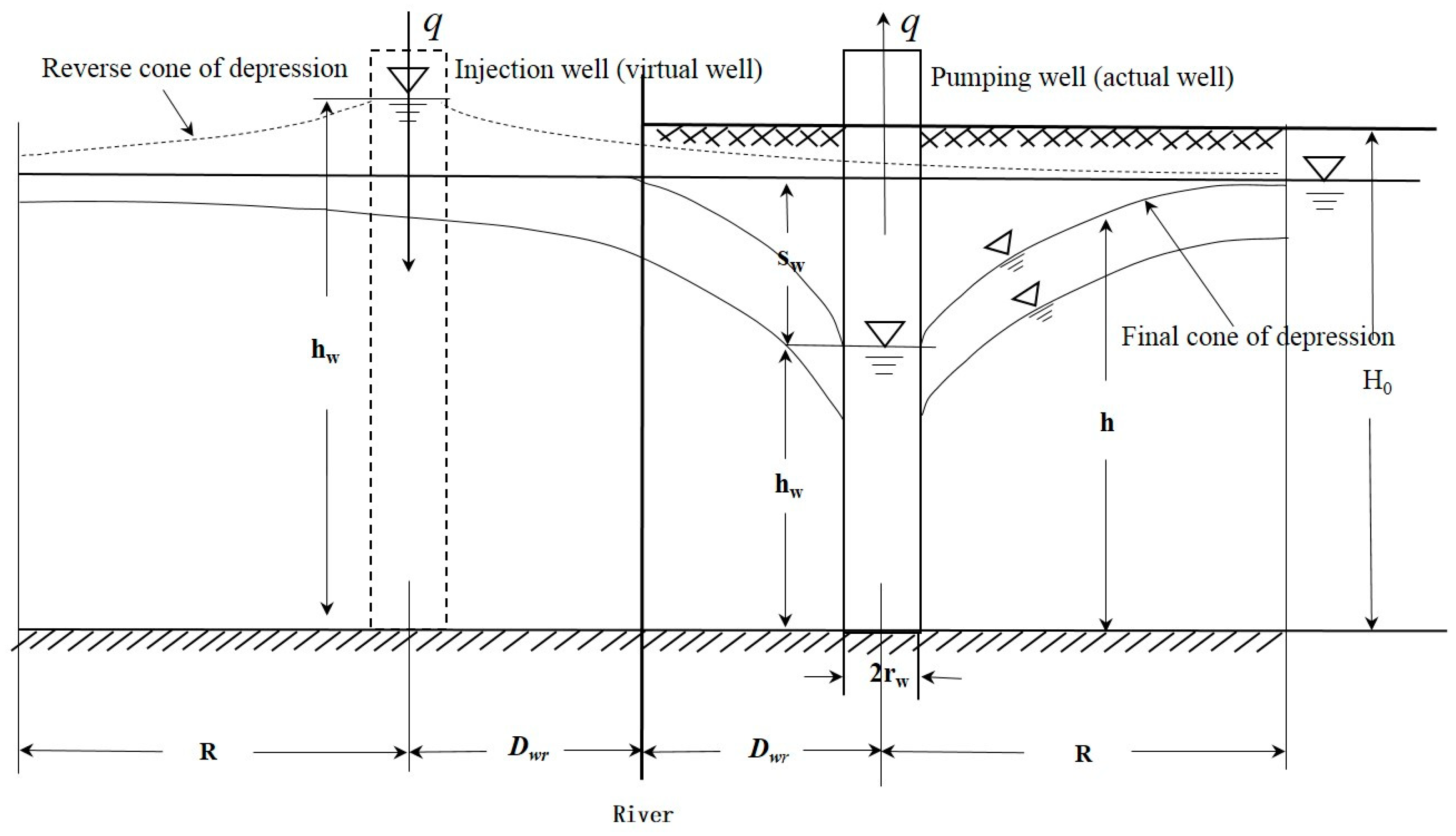
2.2.1. Scenario I: A Single Pumping Well Off-Riverside

Under the condition of a single pumping well off-riverside that was independent of the river, the well could be generalized as an incomplete well in an infinite phreatic aquifer in the horizontal dimension (excluding the upper sealing section). In order to facilitate the calculation, it was assumed that the well meets the Dupuit Hypothesis, that is, the flow line to the well is approximately horizontal, and the contour map of groundwater level was a coaxial cylinder, which was consistent with the passing water section. According to the Dupuit Equation, the water yield of the single well could be calculated as the following:
q = π K ( 2 H 0 s w ) s w l n R r w
where q is the water yield (m3/d); K is the hydraulic conductivity (m/d); H0 is the phreatic aquifer thickness (m); sw is the drawdown of the groundwater level (m); R is the influence radius (m); and rw is the well radius (m).

2.2.2. Scenario II: A Single Pumping Well along a Linear Riverside

Under the condition of a single pumping well along a linear riverside, the river could be determined as a recharge boundary with a specific water level, which could be coped with according to the Mirror-Image Method (Bear, 1979) [32]. To save space, the detailed description of the method was omitted here (the schematic diagram can be seen in Figure 1), which could be referenced to Bear (1979) [32], and the water yield of the single well could be calculated, as the following:
q = π K ( 2 H 0 s w ) s w l g 2 D w r r w
where Dwr is the distance between the well and the river (m); and the other symbols are the same as those in Equation (1).

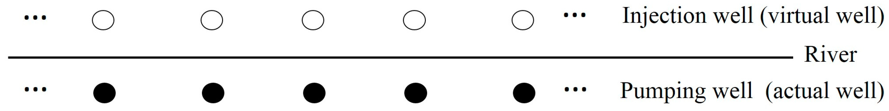
2.2.3. Scenario III: A Well Group along a Linear Riverside

In many practice cases, a set of pumping wells were arranged along a riverside replacing a single well due to the limited water supply capacity of the latter. Thus, the scenario where a well group along a linear riverside was considered in this study. The water supply capacity of this scenario was jointly impacted by the layout of the wells, and the exploitation plan. In this section, we deduced the calculating equations of the exploitation amount of a single well in the well group in addition to that of the well group. Those equations were convenient for the optimization of the layout of the wells and the exploitation plan in the following sections. The Mirror-Image Method was also applicable for this scenario, and the corresponding schematic diagram adapted from that of the scenario with a single well could be seen in Figure 2.
The equation describing the interference between pumping wells could be deduced from Dupuit Equation:
H 0 2 h w 2 = q π K l n R r w
where hw is the groundwater level of the pumping well compared with the bottom of the aquifer, which is valued as the difference value between the aquifer thickness (H0) and the drawdown of the groundwater level (sw) (m); and the other symbols are the same as those of the above equations. The water yield of a pumping well in the well group could be determined by this equation, based on which the total water yield of the well group could be calculated easily if the number of wells was specified.
Superposition calculation could be carried out based on Equation (3) when the total water yield of all the pumping wells were the same [33]:
H 0 2 h i 2 = j = 1 n q π K l n R r j j = 1 n q π K l n R r j + = q π K l n 1 n r j + 1 n r j
where rj+ is the distance between the j injection well and the calculated pumping well (the i well) (m); rj is the distance between two adjacent pumping wells (the i and j well) (m); rj = rw when the pumping well is the calculated pumping well; and the other symbols are the same as those of the above equations.

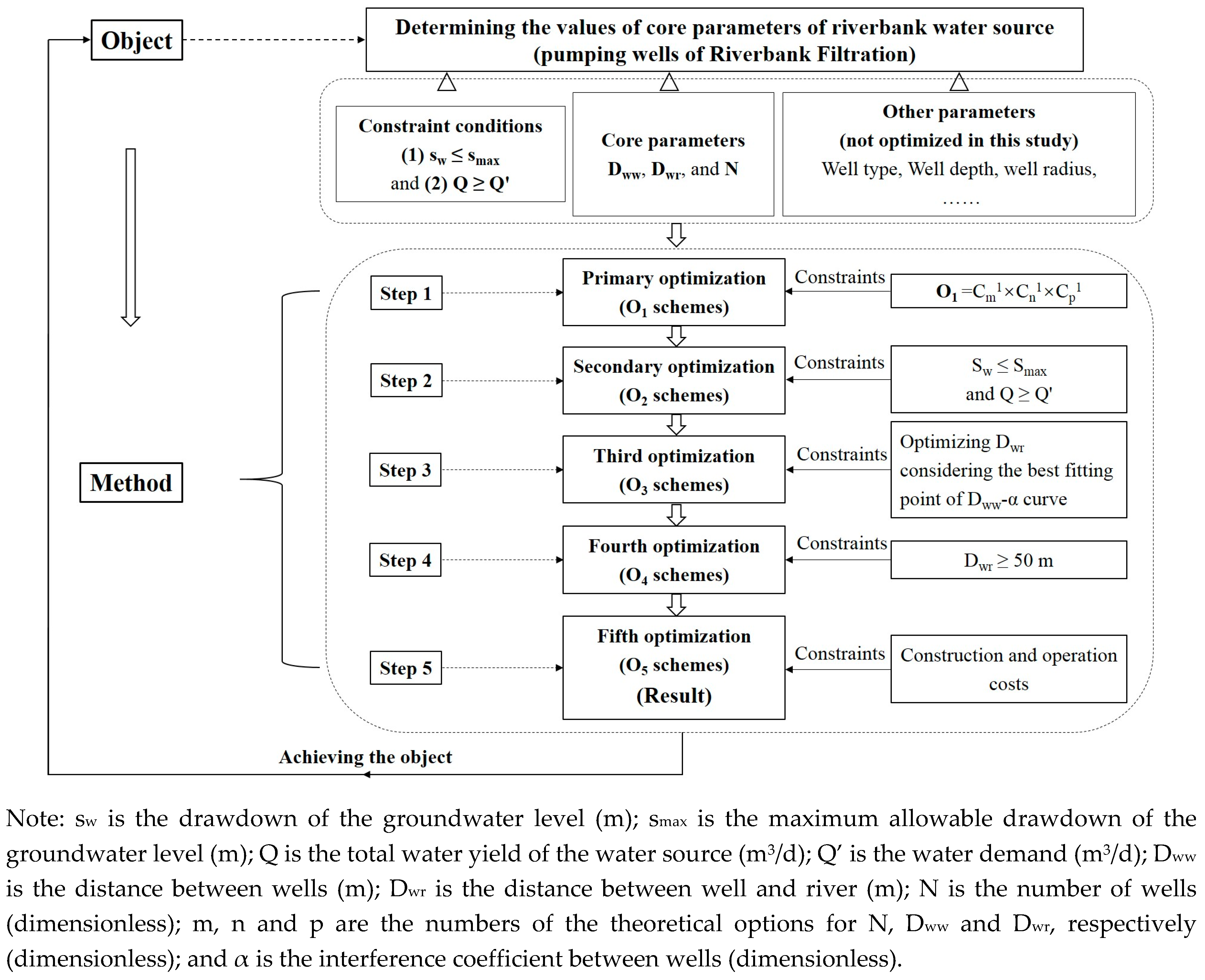
2.3. Method of Design and Optimization of Well Group of Rws

2.3.1. Constraint Conditions

Considering the sustainable exploitation and utilization of RWS, it was essential to avoid causing the persistent decline of the groundwater level and bring an unacceptable negative impact on the ecosystem at the site and around. In this regard, it is common to set one third of the aquifer thickness (H0), as the maximum allowable drawdown of the groundwater level (smax) [33] which should be the upper limit of the drawdown of the groundwater level (sw). The planned water resource exploitation is usually determined jointly by the water demand (Q′), as well as the water supply capacity of the water source (Q) [34]. Sometimes, the construction and operational costs were also taken into account. Taking these factors into account, both sw and Q were selected as the constraint conditions (objective function) as seen in Figure 3. In detail, the results of the design and optimization effort needed to satisfy the two conditions simultaneously: sw ≤ smax, and Q ≥ Q′.

2.3.2. Parameter Design

The layout of the well group directly determined the success of the establishment of the water source. The parameters involved included not only the well type, well depth and well radius (rw), but also the number of wells (N), the distance between wells (Dww) and the distance between well and river (Dwr). It is common to arrange tube wells in a straight line parallel to the river [33], considering it has better stimulation from the recharge from the river. In order to ensure the water intake efficiency, the pumping well was often designed as a completely penetrating well, which penetrated the whole phreatic aquifer in the vertical dimension. As to rw, it is usually determined by the manufacturing technique, and 0.25 m was the most designed value in many regions.
Different from the fixed type and parameters discussed above, it is very complex and difficult to determine the values of N, Dww, and Dwr due to their interactions with each other. Thus, N, Dww, and Dwr were selected as the objective parameters for optimizing through a certain method in this study, and the numbers of the theoretical options for these three parameters were assumed to be m, n, and p, respectively.

2.3.3. Parameter Optimization

In order to facilitate the discussion, the method established in this study was named the “Five-Step Optimizing Method” (Figure 3), and the result schemes obtained by the latter step were the subset of those obtained by the former step (O5 ⊂ O4 ⊂ O3 ⊂ O2 ⊂ O1).
(1) The First Step: The Establishment of all the Possible Schemes (O1)
The first step was to establish the scheme set including all the possible schemes. Considering the numbers of the theoretical options for N, Dww, and Dwr being m, n, and p, respectively, the number of all the possible schemes (O1) equaled the result of C m 1 × C n 1 × C p 1 .
(2) The Second Step: Screening from N
The second step was to compare all the schemes established in O1 and then screen the possible schemes satisfying sw ≤ smax and Q ≥ Q′ simultaneously, forming a scheme set named O2. N depended on Q′ and the water yield of a single well, and the latter was determined by smax. Thus, Q and sw of each scheme should be calculated, followed by the screening of the favorable schemes.
(3) The Third Step: Screening from Dww
The third step was to screen those schemes in O2 with the favorable Dww, which was carried out by establishing the relationship between Dww and α (the interference coefficient between wells) and subsequently, finding the inflection point at the curve. The corresponding Dww value of the inflection point or around was considered to be the favorable Dww [35]. A strong relationship between Dww and α existed, and the greater the Dww was, the smaller α was, which could facilitate obtaining more water yield. However, the greater Dww would increase, the cost including waterline, power transmission system and the corresponding management cost [33]. Thus, it is the designer’s responsibility to minimize Dww as much as possible under the premise of ensuring meeting the water demand [36]. After screening the favorable Dww from O2, the possible schemes further decreased temporarily to form O3.
α referred to the percentage change of the water yield of a single well with disturbance relative to that of a single well without disturbance [35], which could be described as:
α = (q′ − q)/q′
where q is the water yield of a single well with disturbance calculated by Equation (4) (m3/d); and q′ is the water yield of a single well without disturbance calculated by Equation (2) (m3/d).
(4) The Fourth Step: Screening from Dwr
The fourth step was to screen those schemes in O3 with the favorable Dwr. Generally speaking, the smaller the Dwr was, the greater the water yield was, which could increase the efficiency of the water intake engineering. Inversely, the water yield would decrease with the Dwr increasing because the recharge from the river would decrease. Under certain conditions, the impact of river water quality on the well water quality should also be considered, especially in a circumstance of surface water pollution, as pollutants in the RBF usually decreased with the Dwr increasing [37]. After screening the favorable Dwr from O3, the possible schemes further decreased temporarily to form O4, which usually only included two or three schemes or less.
(5) The Fifth (Last) Step: Obtaining the Optimal Option (O5) through Appropriate Consideration of Construction and Operation Costs
More than one scheme was often obtained after the accomplishment of the fourth optimizing step (O4). If that happened, the optimal scheme usually could be screened by appropriately considering the construction and operation cost of the water intake engineering, which was usually not hard to accomplish. Besides, it is also common to encounter other factors that require consideration, such as the available land issue. Thus, it’s occasionally necessary to go further to the fifth (last) step, while more details was omitted here considering the step being relatively strong subjective and maneuverable.

3. Case Study

3.1. Study Area and Generalization

The case study referred to an experimental riverside water source established by the Songhua River, which was located at Harbin City of Heilongjiang Province, northeastern China. The hydrological and hydrogeological investigation, including pumping tests had been carried out during 2017–2018, through which the study area setting had been identified in detail. Limited to the length of this paper, more details were omitted, which could be referenced to Zhu et al. (2019) [2]. Generally speaking, the conditions in the study area met the assumptions of the method with the main parameter values such as K, H0, R, and rw being 50 m/d, 42 m, 200 m and 0.5 m, respectively. As the designed requirement in the method, smax equaled 14 m (one third of H0).

3.2. Water Supply Capacity of the RWS

If a single pumping well was established at the study area without considering the impact of the river, the q (23,056 m3/d ≈ 23,000 m3/d) could be easily determined by the Equation (1). If a single pumping well was established at the study area with simultaneously considering the actual impact of the river, three q values (69,800 m3/d, 61,400 m3/d and 57,400 m3/d) could be easily determined by Equation (2) separately with three designed Dwr values (20 m, 40 m and 60 m). These results showed that the water yields of the single pumping well in the riverside water source were 2.5–3 times as much as that of the single pumping well without the recharge from the river. The variation in multiples was caused by the differences of Dwr, and the smaller the Dwr, the greater both q and the corresponding multiple were. The results showed that Dwr had a great impact on q. As to the scenario of a well group along the riverside, the total water yield was impacted by many parameters complicatedly, which could be seen in the following section.

3.3. The Design and Optimization of the Well Group

3.3.1. Constraint Conditions

As discussed at the beginning of Section 3.1, smax equaled 14 m. Q′ was designed as 2 × 10⁵ m3/d considering the water demand of Harbin City. Thus, the constraint conditions in this case study were: sw ≤ smax = 14 m, and Q ≥ Q′ = 2 × 10⁵ m3/d. The subsequent design and optimization effort was carried out around this goal.

3.3.2. Parameter Design

In this case study, all the pumping wells of the well group of the RWS were designed with the same specifications, considering the convenience of construction and management. The well type (tube well), depth (50 m from the ground to the bottom) and radius (rw, 0.25 m) were directly designed without optimizing. As for those parameters needing optimization (N, Dww and Dwr), the alternative options of the parameter values for optimizing needed to be fixed, considering both the study area setting and the water demand.

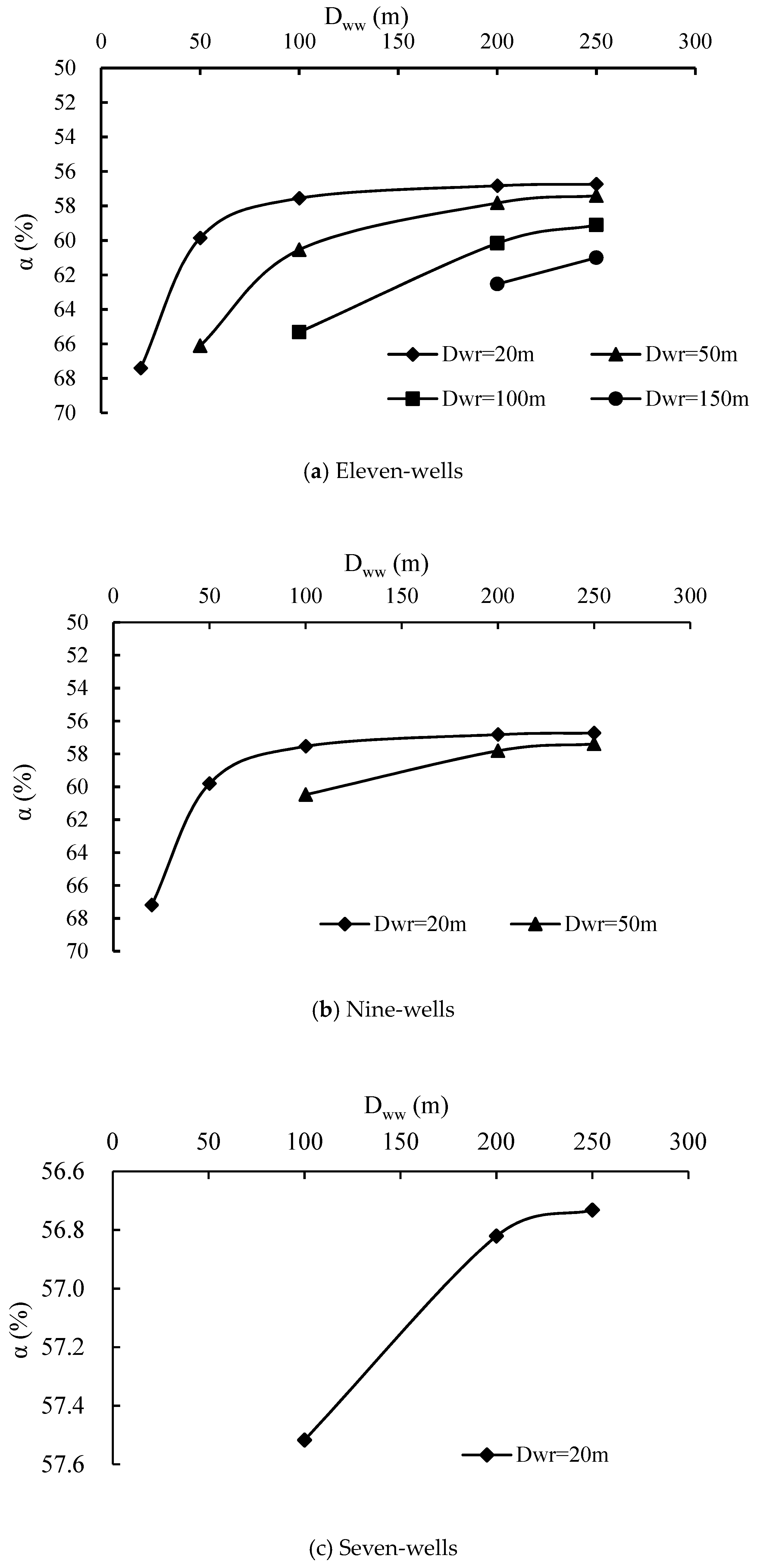
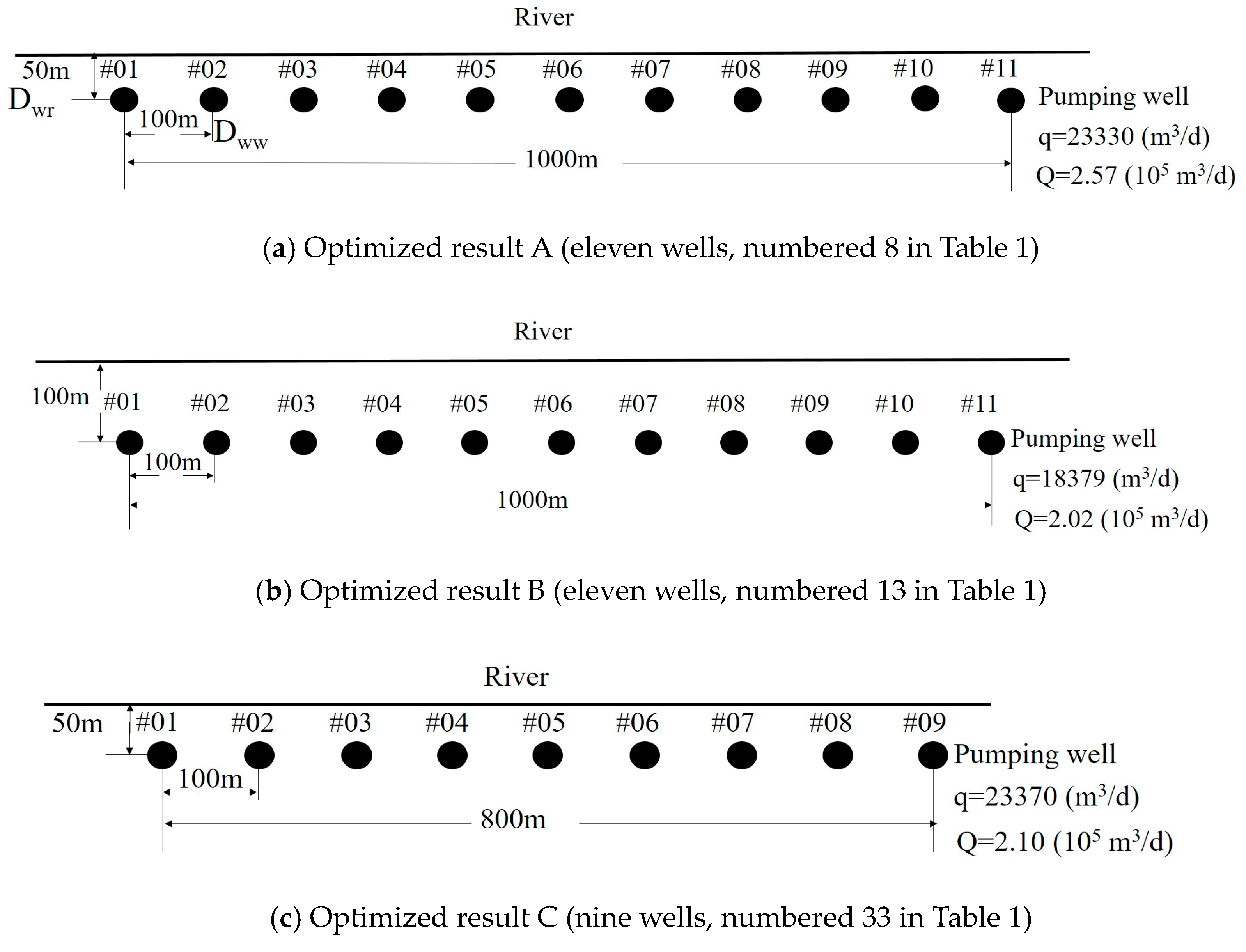
3.3.3. Parameter Optimization

(1) The First Step: The Establishment of all the Possible Schemes (O1)
The alternative values of N were designed as 7, 9, and 11 (m = 3) considering the ratio of Q′/q (8.7) and the possible interaction between wells. The alternative values of Dww were designed as 20 m, 50 m, 100 m, 150 m, and 200 m (n = 5) considering the influence radius and the impact from the river. The alternative values of Dwr were designed as 20 m, 50 m, 100 m, 200 m and 250 m (p = 5) considering the influence radius and the impact from the river. That’s to say, the optimizing effort was to screen the most favorable values set (scheme) of the three parameters from the 75 ( C 3 1 × C 5 1 × C 5 1 ) established schemes (O1) (Table 1) by using the established method. N, Dww, Dwr, q, and Q in Table 1 refer to number of wells, distance between wells, distance between well and river, single well yield, and total yield, respectively, and q was calculated by Equation (4).
(2) The Second Step: Screening from N
The results (Table 1) showed that the favorable schemes (Q ≥ Q′ = 2 × 10⁵ m3/d) for N of 11, 9, and 7 were 14, 8, and 3, respectively, which constituted a new scheme set with 25 possible schemes (O2) (Table 1).
(3) The Third Step: Screening from Dww
All the interference coefficients (α) between wells of schemes in O2 were calculated (Table 2), and correlation diagrams (Figure 4) were drawn to illustrate the relationships between Dww and α with different N and different Dwr. The results showed that α decreased with Dww increasing at the beginning, while decreased almost no longer after the inflection points appeared at the top left corners of all the curves. It suggested that the favorable value of Dww should be around the inflection point, because smaller value would bring more disturbance between wells while greater value would bring more construction, and operation costs considering the occupying space of the wells. Thus, the favorable value of Dww should be 100 m for both eleven-wells and nine-wells, while the same value should be 200 m for seven-wells. The favorable schemes decreased to six (O3) after this optimizing step (Table 2). N, Dww, Dwr, q, q′ and α in Table 2 refer to number of wells, distance between wells, distance between well and river, single well yield, single well yield without interference, and interference coefficient, respectively.
(4) The Fourth Step: Screening from Dwr
In O3 with six schemes (Table 1), the three schemes with Dwr = 20 m were not a wise choice after considering the study area setting carefully, because the distance between the pumping wells and the river was too small to protect the wells from occasional flooding happening in the river. In addition, the safety of the river levee and the possible clogging of the RBF should be also considered. Thus, the schemes numbered 3, 28 and 54 in Table 1 had to be abandoned. So far, only three schemes left in Table 1 constituting O4, which left very little scope to decision maker to select. That is to say, the optimal scheme in fact could be easily singled out from the three options (Figure 5). The drawdown of the groundwater level of the middle pumping well of each scheme is 14.0 m, while the drawdowns of the well at each edge of the three schemes are 12.7 m, 11.7 m, and 12.8 m respectively satisfy the constraint condition. Thus, sometimes the optimizing process could be terminated after this step.
(5) The Fifth (Last) Step: Obtaining the Optimal Option through the Appropriate Consideration of Construction and Operation Costs
In fact, the need to go on to the fifth step is obvious, on occasion, especially when the budget is not adequate, or the riverbed clogging occurs. Out of the three left schemes (Figure 5), the scheme (a) would have to be abandoned considering saving water resource and energy, as the total water yield (Q = 2.57 × 10⁵ m3/d) of it is much more than needed (Q′ = 2 × 10⁵ m3/d). Nevertheless, scheme (a) could also become a choice if the water demand increases. And the scheme (b) would also have to be abandoned considering saving investment, as it has two more pumping wells compared with the scheme (c). Thus, the scheme (c) could be singled out as the final result of the optimizing effort, if other factors are not considered.
However, the scheme (b) is the best choice if 50 m as the distance between the well and the river is considered to be too small to protect against floods and water pollution incidents, or 23,370 m3/d as the pumping yield of each well is considered to be too large to avoid the possible riverbed clogging in practice. That is to say, the final result may switch among the three scenarios considering the establishing investment, the energy consumption, the disaster risk, and the riverbed clogging, etc. Thus, all the three optimized schemes are valuable for the decision maker to choose.

4. Discussion

In this study, we tentatively established a method of design and optimization of pumping wells in riverbank filtration (RBF) by using analytical methods, in which the traditional methods such as the Mirror-Image Method, Dupuit Equation and Interference Well Group Method were jointly adopted. The method assumed that the phreatic aquifer was fully penetrated by the linear river in the vertical dimension, and there was a close hydraulic relation between the surface water and groundwater, both of which had nearly the same natural hydrological curve. The aquifer extended indefinitely in the other three directions and was bounded by an impervious rock at the bottom. The RBF was a homogeneous and isotropic medium, and there was no aquitard or aquiclude around the river. Thus, the model assumed was generally the same as that established by Theis (1941) [38], which was usually considered the simplest mode of surface water-groundwater interactions and rare in practice [31]. The main purpose of this simplification was to facilitate calculation, so we used the Mirror-Image Method in this study, after we proved the applicability [2]. This method was established by Jacob (1979) [32] to calculate the extending of the groundwater level, which is induced by pumping groundwater near the river and the corresponding water supply capacity of the pumping wells. Considering their simplicity, the mode and the corresponding method were often adopted in order to obtain the approximate solutions.
Similar to many other optimizing efforts, the parameters are not independent [39], which makes the optimizing efforts more difficult, especially in the use of analytical methods [40]. The basic hydrogeology tells us that the cone of depression of the groundwater level will continually extend both in the vertical and horizontal dimensions when pumping, unless the aquifer could capture as much as water recharge relative to the water yield [41]. Thus, the cones of depression of the different pumping wells will interact with each other if the distance between wells is not far enough [42], which will inevitably affect the efficiency of the pumping wells through decreasing the water capacity of a single well [43]. However, the cost will increase considering the water supply network and the power supply line if the distance is too far, especially when the number of the pumping wells are great [44]. Thus, it is an art to design the distance between wells, especially when there are many wells [45]. More than that, the recharge of the pumping well of RBF is usually much more than that of off-riverside because the former could capture a portion of river water [2]. Thus, the interaction of cones of depression of different wells will be more complex, which further complicates the design art of the distance of wells. As to the river-groundwater interaction, the river water captured by the pumping well is directly determined by the distance of the well and the river if the other parameters are fixed [46]. It is better to design a smaller value to the distance between well and river, only if the water quantity is considered in the engineering. However, it is not favorable for the effectiveness of the RBF as a pre-treatment measure of water [47]. Furthermore, it is also not favorable for protecting the wells from possible river flooding and water pollution, which will pose significant impact on the safety of the social water supply. The water quality is obviously also an important issue considering both the pre-treatment function of the RBF and the subsequent design of the post-treatment of the plant. The water quality issue was not considered quantitatively in this study, mainly because we considered that, the optimal scheme considering both the water quantity and quality of the pumping wells should only be singled out from the optional schemes only considering the water quantity, which was obtained from the optimizing method established in this study. That is to say, the design and optimization effort made in this study is the basis of considering the water quality issue, based on which the optimal scheme can be determined for both water quantity and quality.
River-groundwater interactions are at the core of a wide range of major contemporary challenges [48], out of which the provision of high-quality drinking water in sufficient quantities is without doubt the most important because it involves water demand of human society. Riverbank filtration (RBF) has been used for many decades widely worldwide especially in Europe, the United States and some Asian countries (China, India, Japan, South Korea, etc.) to provide drinking water [1,49]. However, the existing RBF comprehension mainly depends on practical understandings, and no standards have been developed to guide the optimization of the RBF design [50]. Thus, we have good reason to believe that more design and optimization efforts on RBF considering water quantity and quality or both will be carried out in the following periods.

5. Conclusions

An optimizing method named Five-Step Optimizing Method was established systematically by us aiming to improve the design effort of engineering parameters of water pumping wells in riverbank filtration. The maximum allowable drawdown of groundwater level (smax) and the water demand of society (Q′) jointly constituted the constraint conditions. Three parameters including the number of wells (N), the distance between wells (Dww) and the distance between well and river (Dwr) could be optimized through the established method step-by-step by screening the alternative values beforehand designed for the parameters. The interference between wells was found to be a decisive factor, which had a significant impact on the design and optimization effort of all the three parameters. Dwr was another decisive factor impacting the recharge from the river, and subsequently the well water yield. The optimized result would sometimes supply the decision maker with more than one optional scheme for selecting, while it is not yet difficult in practice to single out the optimal one considering both the field setting and the water demand.
A case study was carried out along the Songhua River in Harbin City of Heilongjiang Province of northeast China, whose setting generally met the assumptions of the method, aiming to illustrate the application and simultaneously verify the applicability of the method. Three schemes with different parameter values obtained from the optimizing method could meet the constraint conditions (smax = 14 m; and Q′ = 2 × 10⁵ m3/d), out of which the optimal option had the parameters: N = 9; Dww = 100 m; and Dwr = 50 m. Meanwhile, the other two schemes were valuable in certain circumstances, which should also be referred to the decision maker. This case study proved that the established method was applicable.
Admittedly, the method established in this study has some limitations, especially in the limitations of the assumptions. At the very least, however, this effort provides a relatively simple and operational approach to relevant practices and decisions.

Author Contributions

Conceptualization, Y.Z. (Yuanzheng Zhai); Methodology, Y.Z. (Yuanzheng Zhai) and J.Z.; Formal analysis, Y.J. and J.Z.; Investigation, Y.Z. (Yaguang Zhu) and Q.D.; Data curation, J.Z.; Writing—original draft, Y.J. and J.Z.; Writing—review & editing, Y.Z. (Yuanzheng Zhai); Supervision, Y.T.; Funding acquisition, Y.Z. (Yuanzheng Zhai) and Y.T.

Funding

This work was supported by the National Natural Science Foundation of China (No. 41877174 and 41877355), and the Major Science and Technology Program for Water Pollution Control and Treatment (2018ZX07101005-04).

Conflicts of Interest

The authors declare no conflict of interest. The funders had no role in the design of the study; in the collection, analyses, or interpretation of data; in the writing of the manuscript; or in the decision to publish the results.

References

  1. Hu, B.; Teng, Y.; Zhai, Y.; Zuo, R.; Li, J.; Chen, H. Riverbank filtration in China: A review and perspective. J. Hydrol. 2016, 541, 914–927. [Google Scholar] [CrossRef]
  2. Zhu, Y.; Zhai, Y.; Du, Q.; Teng, Y.; Wang, J.; Yang, G. The impact of well drawdowns on the mixing process of river water and groundwater and water quality in a riverside well field, Northeast China. Hydrol. Process. 2019. [Google Scholar] [CrossRef]
  3. Yin, W.; Teng, Y.; Zhai, Y.; Hu, L.; Zhao, X.; Zhang, M. Suitability for developing riverside groundwater sources along Songhua River, Northeast China. Hum. Ecol. Risk Assess. 2018, 8, 2088–2100. [Google Scholar] [CrossRef]
  4. Hester, E.T.; Cardenas, M.B.; Haggerty, R.; Apte, S.V. The importance and challenge of hyporheic mixing. Water Resour. Res. 2017, 53, 3565–3575. [Google Scholar] [CrossRef]
  5. Steen, C.; Vitaly, A.Z.; Daniel, M.T. On the use of analytical solutions to design pumping tests in leaky aquifers connected to a stream. J. Hydrol. 2010, 381, 341–351. [Google Scholar]
  6. Baalousha, H.M. Drawdown and stream depletion induced by a nearby pumping well. J. Hydrol. 2012, 466–467, 47–59. [Google Scholar] [CrossRef]
  7. Jin, M.; Xian, Y.; Liu, Y. Disconnected stream and groundwater interaction: A review. Adv. Water Sci. 2017, 28, 149–160, (In Chinese with English abstract). [Google Scholar]
  8. Lu, C.; Shu, C.; Chen, X. Numerical analysis of the impacts of bedform on hyporheic exchange. Adv. Water Sci. 2012, 23, 789–795, (In Chinese with English abstract). [Google Scholar]
  9. Pholkern, K.; Srisuk, K.; Grischek, T.; Soares, M.; Schäfer, S.; Archwichai, L.; Saraphirom, P.; Pavelic, P.; Wirojanagud, W. Riverbed clogging experiments at potential river bank filtration sites along the Ping River, Chiang Mai, Thailand. Environ. Earth Sci. 2015, 73, 7699–7709. [Google Scholar] [CrossRef]
  10. Grischek, T.; Bartak, R. Riverbed clogging and sustainability of riverbank filtration. Water 2016, 12, 604. [Google Scholar] [CrossRef]
  11. Shaymaa, M.; Arifah, B.; Zainal, A.A.; Saim, S. Review of the role of analytical modelling methods in riverbank filtration system. J. Teknol. 2014, 1, 59–69. [Google Scholar]
  12. Knapp, J.L.A.; Cirpka, O.A. Determination of hyporheic travel-time distributions and other parameters from concurrent conservative and reactive tracer tests by local-in-global optimization. Water Resour. Res. 2017, 53, 4984–5001. [Google Scholar] [CrossRef]
  13. Xie, Y.; Peter, G.C.; Craig, T.S.; Zheng, C. On the limits of heat as a tracer to estimate reach-scale river-aquifer exchange flux. Water Resour. Res. 2015, 51, 7401–7416. [Google Scholar] [CrossRef] [Green Version]
  14. Stefania, G.A.; Rotiroti, M.; Fumagalli, L.; Simonetto, F.; Capodaglio, P.; Zanotti, C.; Bonomi, T. Modeling groundwater/surface-water interactions in an Alpine valley (the Aosta Plain, NW Italy): The effect of groundwater abstraction on surface-water resources. Hydrogeol. J. 2018, 26, 147–162. [Google Scholar] [CrossRef]
  15. Wen, Z.; Zhan, H.; Wang, Q.; Liang, X.; Ma, T.; Chen, C. Well hydraulics in pumping tests with exponentially decayed rates of abstraction in confined aquifers. J. Hydrol. 2017, 548, 40–45. [Google Scholar] [CrossRef]
  16. Xie, X.; Johnson, T.M.; Wang, Y.; Lundstrom, C.C.; Ellis, A.; Wang, X.; Duan, M.; Li, J. Pathways of arsenic from sediments to groundwater in the hyporheic zone: Evidence from an iron isotope study. J. Hydrol. 2014, 511, 509–517. [Google Scholar] [CrossRef]
  17. Cardenas, M.B. Hyporheic zone hydrologic science: A historical account of its emergence and a prospectus. Water Resour. Res. 2015, 51, 3601–3616. [Google Scholar] [CrossRef] [Green Version]
  18. Gökçe, Ş.; Ayvaz, M.T. Evaluation of Harmony Search and Differential Evolution Optimization Algorithms on Solving the Booster Station Optimization Problems in Water Distribution Networks; Springer: Cham, Switzerland, 2015; pp. 245–261. [Google Scholar]
  19. Miracapillo, C.; Morel-Seytoux, H.J. Analytical solutions for stream-aquifer flow exchange under varying head asymmetry and river penetration: Comparison to numerical solutions and use in regional groundwater models. Water Resour. Res. 2014, 50, 7430–7444. [Google Scholar] [CrossRef] [Green Version]
  20. Hamann, E.; Stuyfzand, P.J.; Greskowiak, J.; Timmer, H.; Massmann, G. The fate of organic micropollutants during long-term/long-distance river bank filtration. Sci. Total Environ. 2015, 545–546, 629–640. [Google Scholar] [CrossRef] [PubMed]
  21. Salamon, E.; Goda, Z. Coupling riverbank filtration with reverse osmosis may favor short distances between wells and riverbanks at RBF sites on the River Danube in Hungary. Water 2019, 11, 113. [Google Scholar] [CrossRef]
  22. Mantoglou, A.; Papantoniou, M.; Giannoulopoulos, P. Management of coastal aquifers based on nonlinear optimization and evolutionary algorithms. J. Hydrol. 2004, 297, 209–228. [Google Scholar] [CrossRef]
  23. Jin-Yong, L.; Kang-Kun, L.; Se-Yeong, H.; Yongcheol, K. Fifty years of groundwater science in Korea: A review and perspective. Geosci. J. 2017, 6, 951–969. [Google Scholar]
  24. Tian, G.L.; Chang, J.B.; Wang, W. Application of analytical method to the calculation of groundwater permissible mining capacity. J. Pearl River 2016, 10, 1–7, (In Chinese with English abstract). [Google Scholar]
  25. Hansen, A.K.; Franssen, H.J.H.; Bauer-Gottwein, P.; Madsen, H.; Rosbjerg, D.; Kaiser, H.P. Well field management using multi-objective optimization. Water Resour. Manag. 2013, 27, 629–648. [Google Scholar] [CrossRef]
  26. Polomčić, D.; Hajdin, B.; Stevanović, Z.; Bajić, D.; Hajdin, K. Groundwater management by riverbank filtration and an infiltration channel: The case of Obrenovac, Serbia. Hydrogeol. J. 2013, 21, 1519–1530. [Google Scholar] [CrossRef]
  27. Lee, E.; Hyun, Y.; Lee, K.K.; Shin, J. Hydraulic analysis of a radial collector well for riverbank filtration near Nakdong River, South Korea. Hydrogeol. J. 2012, 20, 575–589. [Google Scholar] [CrossRef]
  28. AbdelFattah, A.; Langford, R.; SchulzeMakuch, D. Applications of particle-tracking techniques to bank infiltration: A case study from El Paso, Texas, USA. Environ. Geol. 2008, 55, 505–515. [Google Scholar] [CrossRef]
  29. Fragoso, T.; Cunha, M.D.C.; LoboFerreira, J.P. Optimal pumping from Palmela water supply wells (Portugal) using simulated annealing. Hydrogeol. J. 2009, 17, 1935–1948. [Google Scholar] [CrossRef]
  30. Haas, R.; Opitz, R.; Grischek, T.; Otter, P. The AquaNES Project: Coupling riverbank filtration and ultrafiltration in drinking water treatment. Water 2019, 11, 18. [Google Scholar] [CrossRef]
  31. Hunt, B. Unsteady stream depletion from ground water pumping. Ground Water 1999, 37, 98–102. [Google Scholar] [CrossRef]
  32. Bear, J. Hydraulics of Groundwater; McGraw-Hill: New York, NY, USA, 1979. [Google Scholar]
  33. Wen, C.; Dong, W.; Cui, G.; Liu, Y.; Su, X. Application of analytical methods to determination of the exploitation scheme of a wellfield at riverside. Hydrogeol. Eng. Geol. 2017, 3, 19–26, (In Chinese with English abstract). [Google Scholar]
  34. Gaur, S.; Mimoun, D.; Graillot, D. Advantages of the analytic element method for the solution of groundwater management problems. Hydrol. Process. 2011, 25, 3426–3436. [Google Scholar] [CrossRef]
  35. Li, Y.; Li, Z. The analytical method for rationally distributing interference well group. J. Xi’an Coll. Geol. 1997, S1, 47–50, (In Chinese with English abstract). [Google Scholar]
  36. Katsifarakis, K.L. Groundwater pumping cost minimization-an analytical approach. Water Resour. Manag. 2008, 22, 1089–1099. [Google Scholar] [CrossRef]
  37. Hoehn, E.; Scholtis, A. Exchange between a river and groundwater, assessed with hydrochemical data. Hydrol. Earth Syst. Sci. 2011, 15, 983–988. [Google Scholar] [CrossRef] [Green Version]
  38. Theis, C.V. The effect of a well on the flow of a nearby stream. Trans. Am. Geophys. Union 1941, 22, 734–738. [Google Scholar] [CrossRef]
  39. Wang, P.; Sergey, P.P.; Vsevolod, M.S. Optimum experimental design of a monitoring network for parameter identification at riverbank well fields. J. Hydrol. 2015, 523, 531–541. [Google Scholar] [CrossRef] [Green Version]
  40. Hund-Der, Y.; Ya-Chi, C. Recent advances in modeling of well hydraulics. Adv. Water Resour. 2013, 51, 27–51. [Google Scholar]
  41. Wang, Y.; Zheng, C.; Ma, R. Review: Safe and sustainable groundwater supply in China. Hydrogeol. J. 2018, 26, 1301–1324. [Google Scholar] [CrossRef]
  42. Holzbecher, E. Analytical solution for well design with respect to discharge ratio. Groundwater 2013, 1, 128–134. [Google Scholar] [CrossRef] [PubMed]
  43. Zhang, Y.; Susan, H.; Finsterle, S. Factors governing sustainable groundwater pumping near a river. Groundwater 2011, 3, 432–444. [Google Scholar] [CrossRef] [PubMed]
  44. Mojtaba, S.; Javad, D.S.M. Optimum pumping well placement and capacity design for a groundwater lowering system in urban areas with the minimum cost objective. Water Resour. Manag. 2017, 13, 4207–4225. [Google Scholar]
  45. Rao, S.V.N.; Sudhir, K.; Shashank, S.; Sinha, S.K.; Manju, S. Optimal pumping from skimming wells from the Yamuna River flood plain in north India. Hydrogeol. J. 2007, 6, 1157–1167. [Google Scholar] [CrossRef]
  46. Hantush, M.S. Wells near streams with semipervious beds. J. Geophys. Res. 1965, 70, 2829–2838. [Google Scholar] [CrossRef]
  47. Van Driezum, I.H.; Derx, J.; Oudega, T.J.; Zessner, M.; Naus, F.L.; Saracevic, E.; Kirschner, A.K.T.; Sommer, R.; Farnleitner, A.H.; Blaschke, A.P. Spatiotemporal resolved sampling for the interpretation of micropollutant removal during riverbank filtration. Sci. Total Environ. 2019, 649, 212–223. [Google Scholar] [CrossRef] [PubMed]
  48. Brunner, P.R.; Therrien, P.R.; Simmons, C.T.; Franssen, H.J.H. Advances in understanding river-groundwater interactions. Rev. Geophys. 2017, 3, 818–854. [Google Scholar] [CrossRef]
  49. Ray, C. Worldwide potential of riverbank filtration. Clean Technol. Environ. Policy 2008, 10, 223–225. [Google Scholar] [CrossRef]
  50. Ahmed, K.A.A. Review on river bank filtration as an in situ water treatment process. Clean Technol. Environ. Policy 2017, 2, 349–359. [Google Scholar] [CrossRef]
Figure 1. Diagram of the Mirror-Image method for a specified-head recharge boundary (river in special).
Water 11 00418 g001
Figure 2. Schematic of Mirror-Image Method of the scenario of a well group paralleling to the river line.
Water 11 00418 g002
Figure 3. Roadmap of the optimizing method (Five-Step Optimizing Method) established in the study.
Water 11 00418 g003
Figure 4. Relationships between Dww and α of pumping wells.
Water 11 00418 g004
Figure 5. Schemes obtained from the fourth optimizing step.
Water 11 00418 g005
Table 1. All possible schemes and the corresponding results of each optimizing step.
No.NDww (m)Dwr (m)q (m3/d)Q (×105 m3/d)Result *
111202022,7542.50AB
211502028,0223.08AB
3111002029,6293.26ABC
4112002030,1353.32AB
5112502030,1993.32AB
611205014,0211.54A
711505020,0382.20AB
8111005023,3302.57ABCD
9112005024,9352.74AB
10112505025,1852.77AB
11112010095551.05A
12115010014,4991.60A
131110010018,3792.02ABCDE
141120010021,1112.32AB
151125010021,6702.38AB
16112015077630.85A
17115015011,7721.30A
181110015015,5231.71A
191120015018,7232.06AB
201125015019,4852.14AB
21112020067850.75A
22115020010,1351.12A
231110020013,61014.97A
241120020016,9741.87A
251125020017,8581.96A
269202022,9022.06AB
279502028,0582.53AB
2891002029,6392.67ABC
2992002030,1372.71AB
3092502030,2012.72AB
319205014,3431.29A
329505020,1531.81A
3391005023,3702.10ABCDE
3492005024,9462.25AB
3592505025,1932.27AB
3692010010,0200.90A
3795010014,7271.33A
38910010018,4761.66A
39920010021,1441.90A
40925010021,6921.95A
4192015082870.75A
4295015012,0851.09A
43910015015,6751.41A
44920015018,7791.70A
45925015019,5251.76A
4692020073330.66A
4795020010,5070.95A
48910020013,8111.24A
49920020017,0561.54A
50925020017,9171.61A
517202023,1411.62A
527502028,1171.97A
5371002029,6562.08AB
5472002030,1422.11ABC
5572502030,2042.11AB
567205014,8571.04A
577505020,3381.42A
5871005023,4331.64A
5972005024,9641.75A
6072505025,2041.76A
6172010010,7380.75A
6275010015,0921.06A
63710010018,6311.30A
64720010021,1961.48A
65725010021,7271.52A
6672015090770.64A
6775015012,5770.88A
68710015015,9181.11A
69720015018,8711.32A
70725015019,5881.37A
7172020081480.57A
7275020011,0860.78A
73710020014,1320.99A
74720020017,1881.20A
75725020018,0111.26A
* A: the result of the first optimizing step; AB: the result of the second optimizing step; ABC: the result of the third optimizing step; ABCD: the result of the fourth optimizing step; and ABCDE: the result of the fifth (last) optimizing step.
Table 2. Interference coefficient of wells.
No.NDww (m)Dwr (m)q (m3/d)q′ (m3/d)α (%)
111202022,753.569,805.667.40
211502028,021.869,805.659.86
3111002029,629.269,805.657.55
4112002030,134.769,805.656.83
5112502030,199.269,805.656.74
611505020,038.259,130.166.11
7111005023,330.259,130.160.54
8112005024,934.759,130.157.83
9112505025,185.259,130.157.41
101110010018,379.052,998.765.32
111120010021,111.352,998.760.17
121125010021,669.952,998.759.11
131120015018,722.649,967.862.53
141125015019,485.149,967.861.00
159202022,901.569,805.667.19
169502028,058.269,805.659.81
1791002029,639.469,805.657.54
1892002030,137.369,805.656.83
1992502030,200.969,805.656.74
2091005023,369.659,130.160.48
2192005024,946.059,130.157.81
2292505025,192.659,130.157.39
2371002029,655.869,805.657.52
2472002030,141.669,805.656.82
2572502030,203.669,805.656.73

