Modelling of Soil Erosion and Accumulation in an Agricultural Landscape—A Comparison of Selected Approaches Applied at the Small Stream Basin Level in the Czech Republic


Abstract
:
1. Introduction
2. Materials and Methods
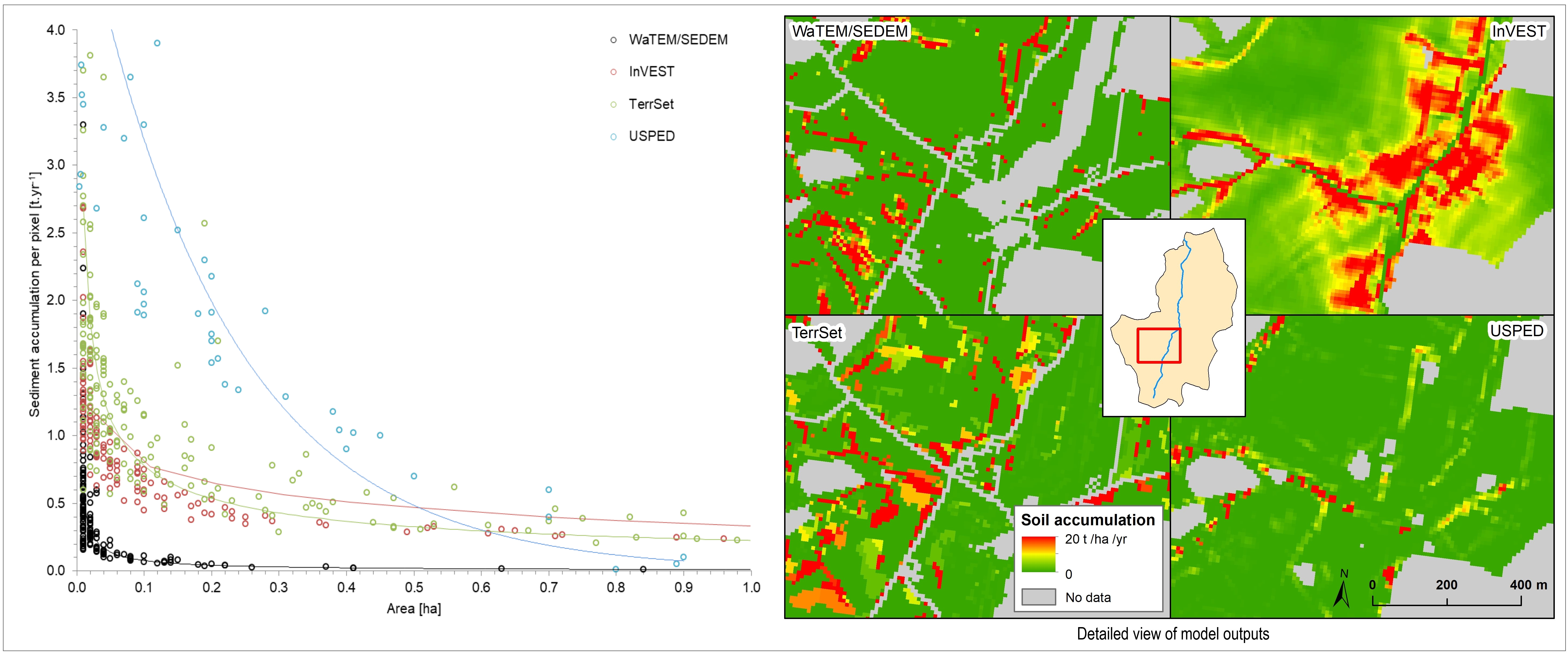
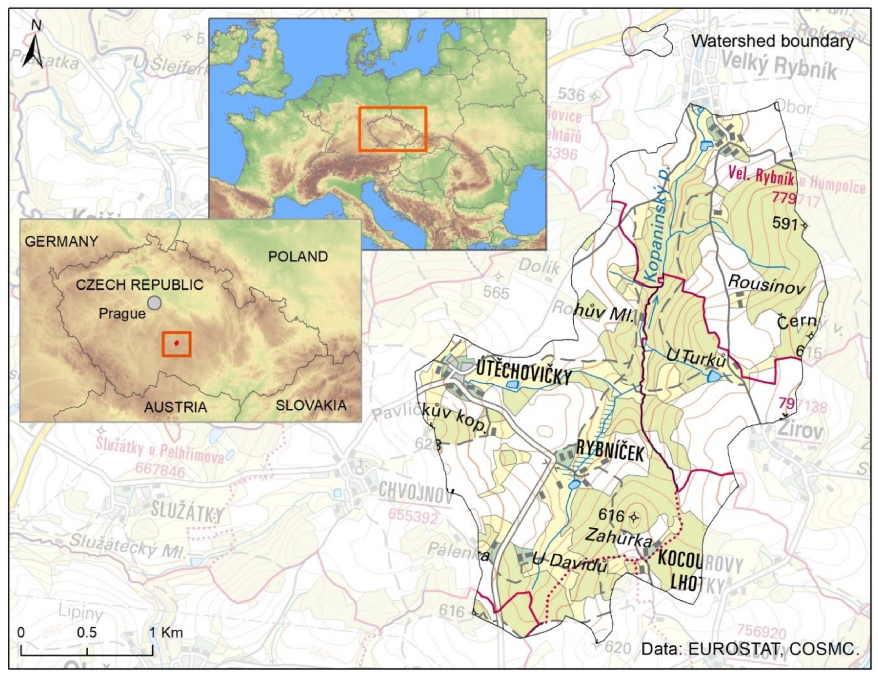
2.1. Case Study Area
2.2. Data Sources
2.3. Approaches Used to Soil Loss and Sediment Accumulation Modelling
2.3.1. InVEST
2.3.2. USPED
2.3.3. TerrSet
2.3.4. WaTEM/SEDEM
3. Results
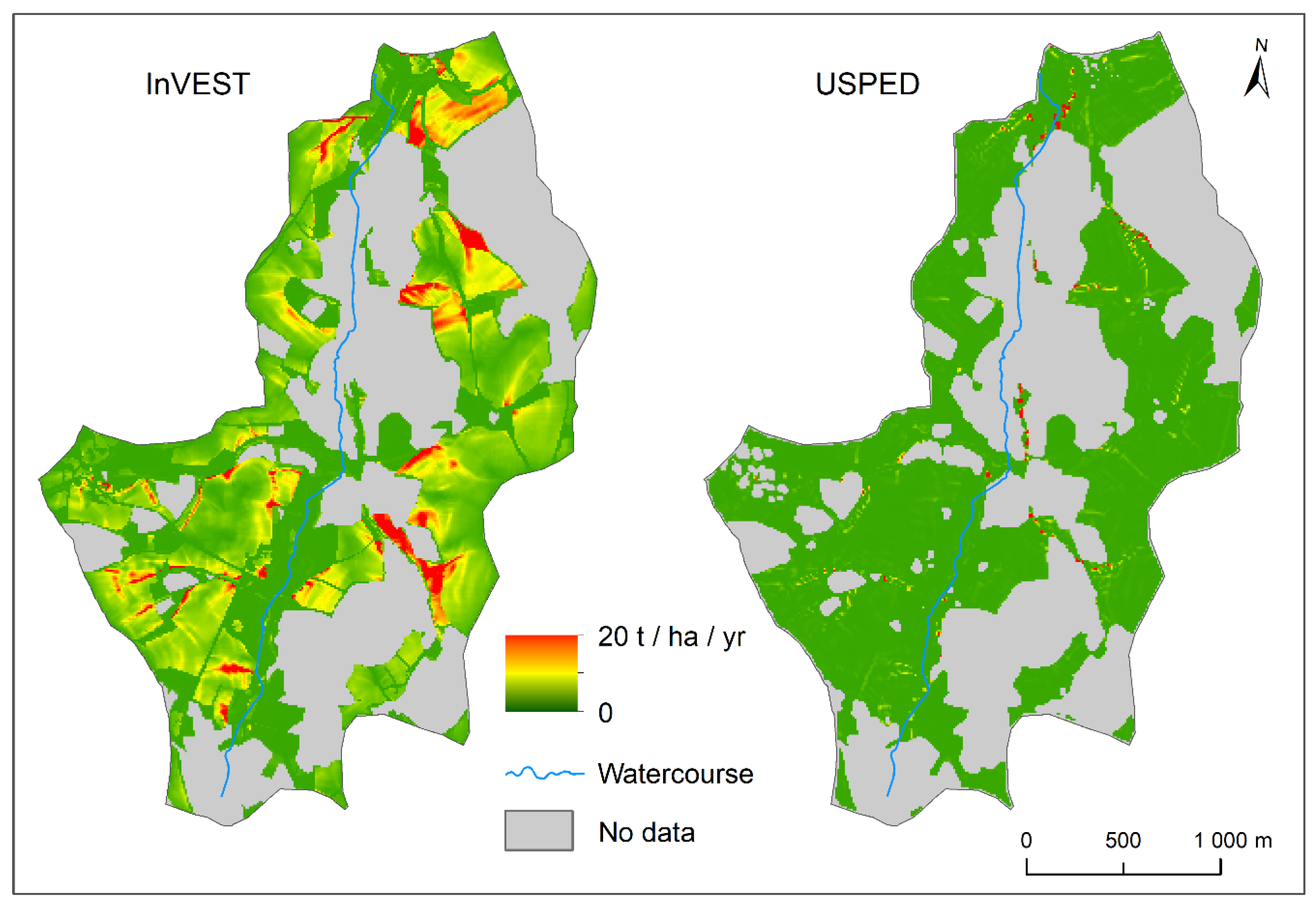
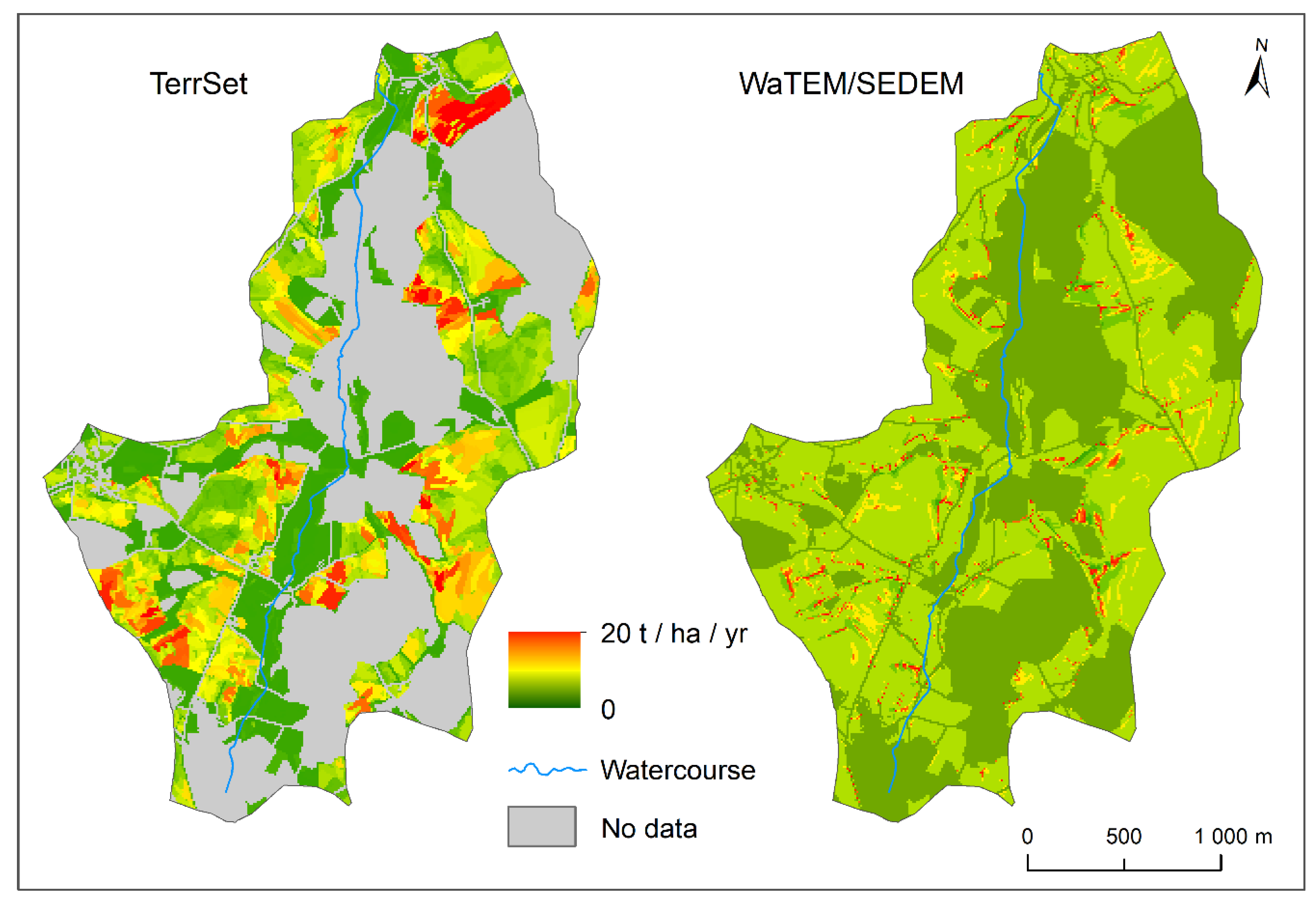
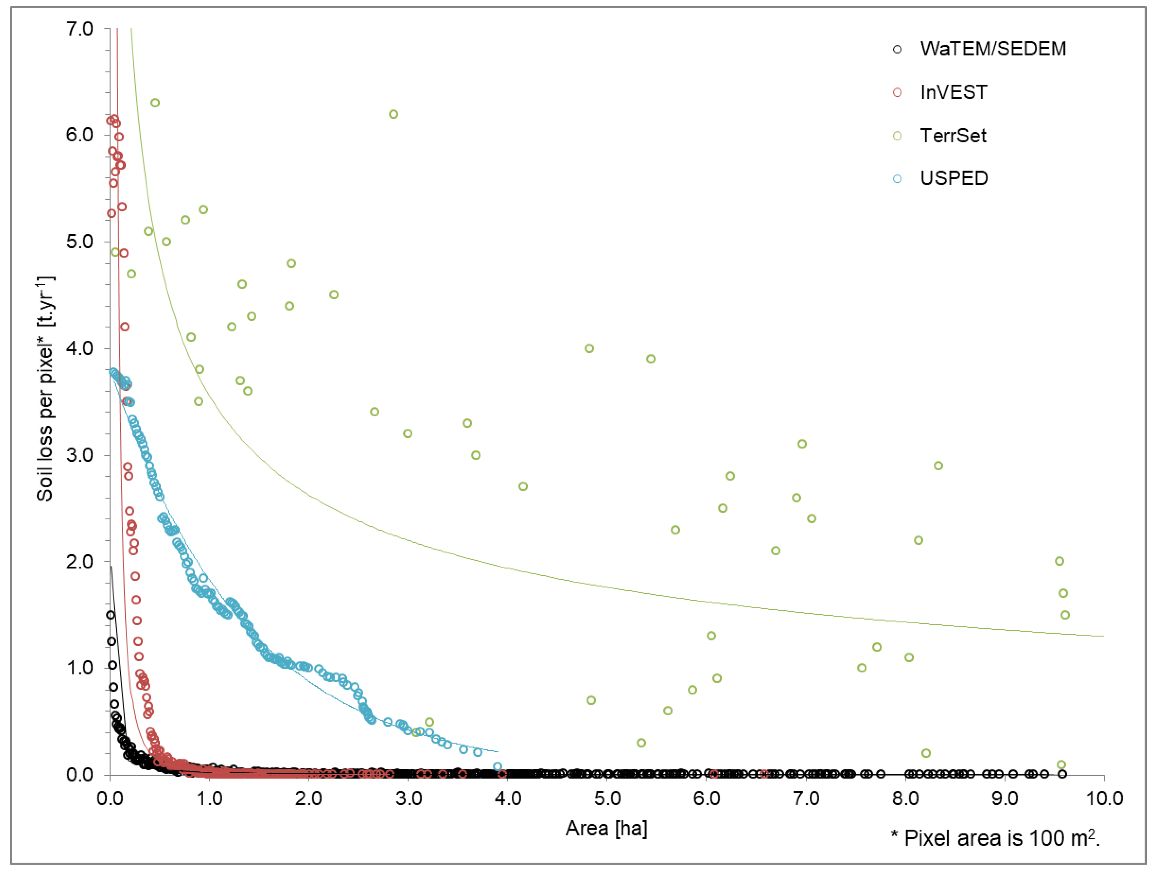
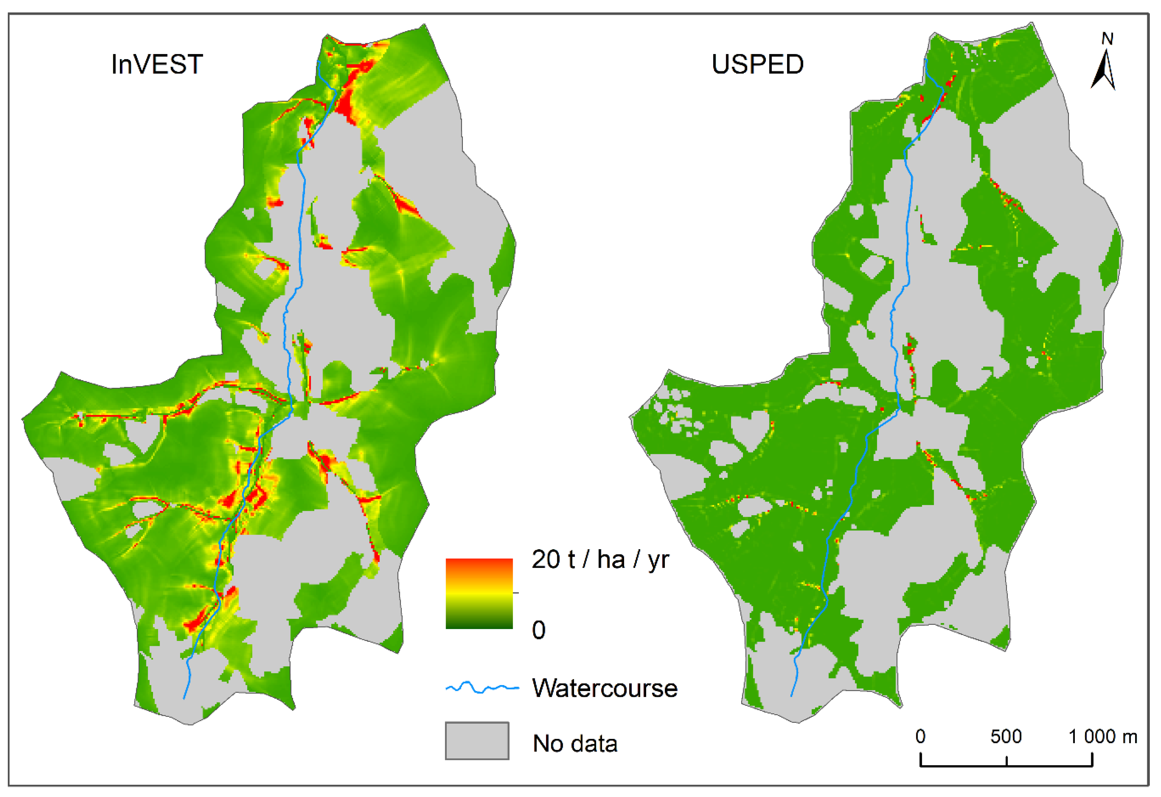
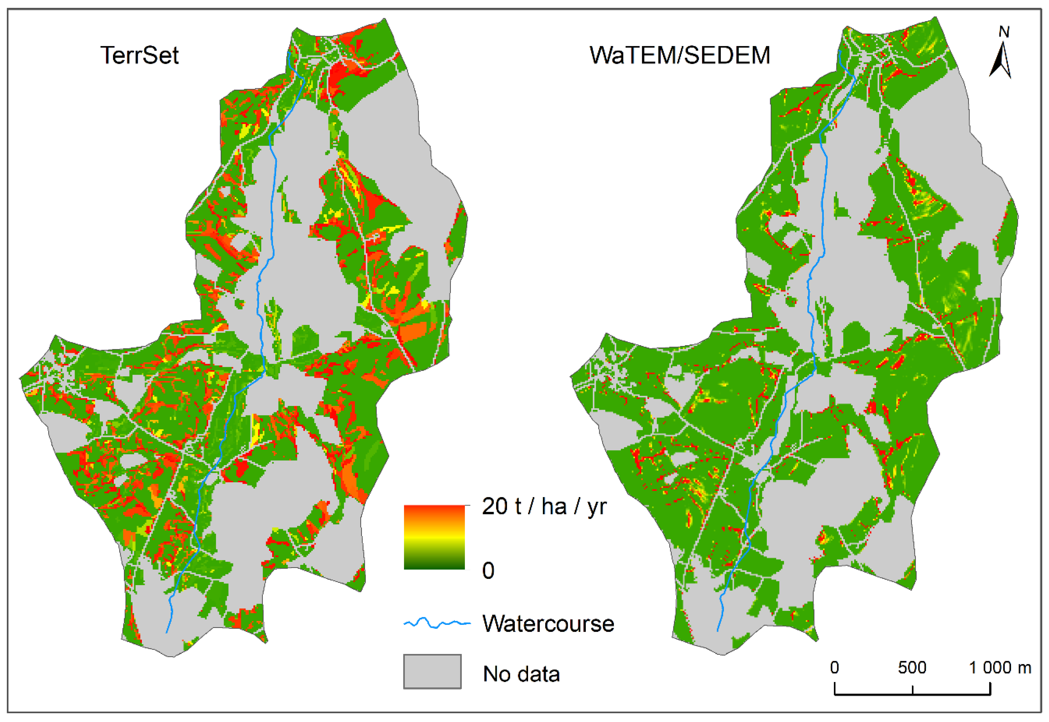
3.1. Analysis of Soil Loss Caused by Water Erosion
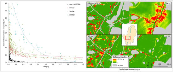
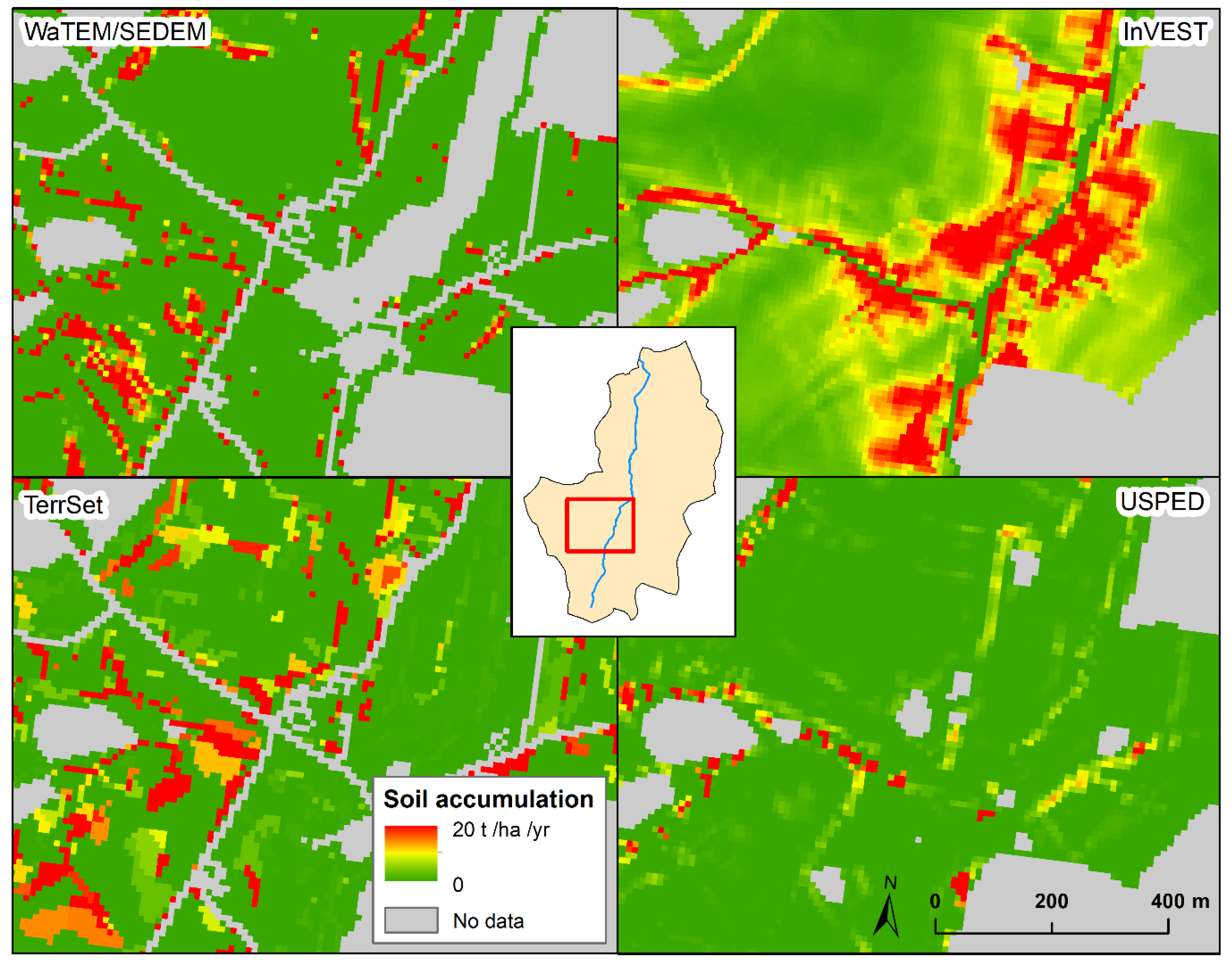
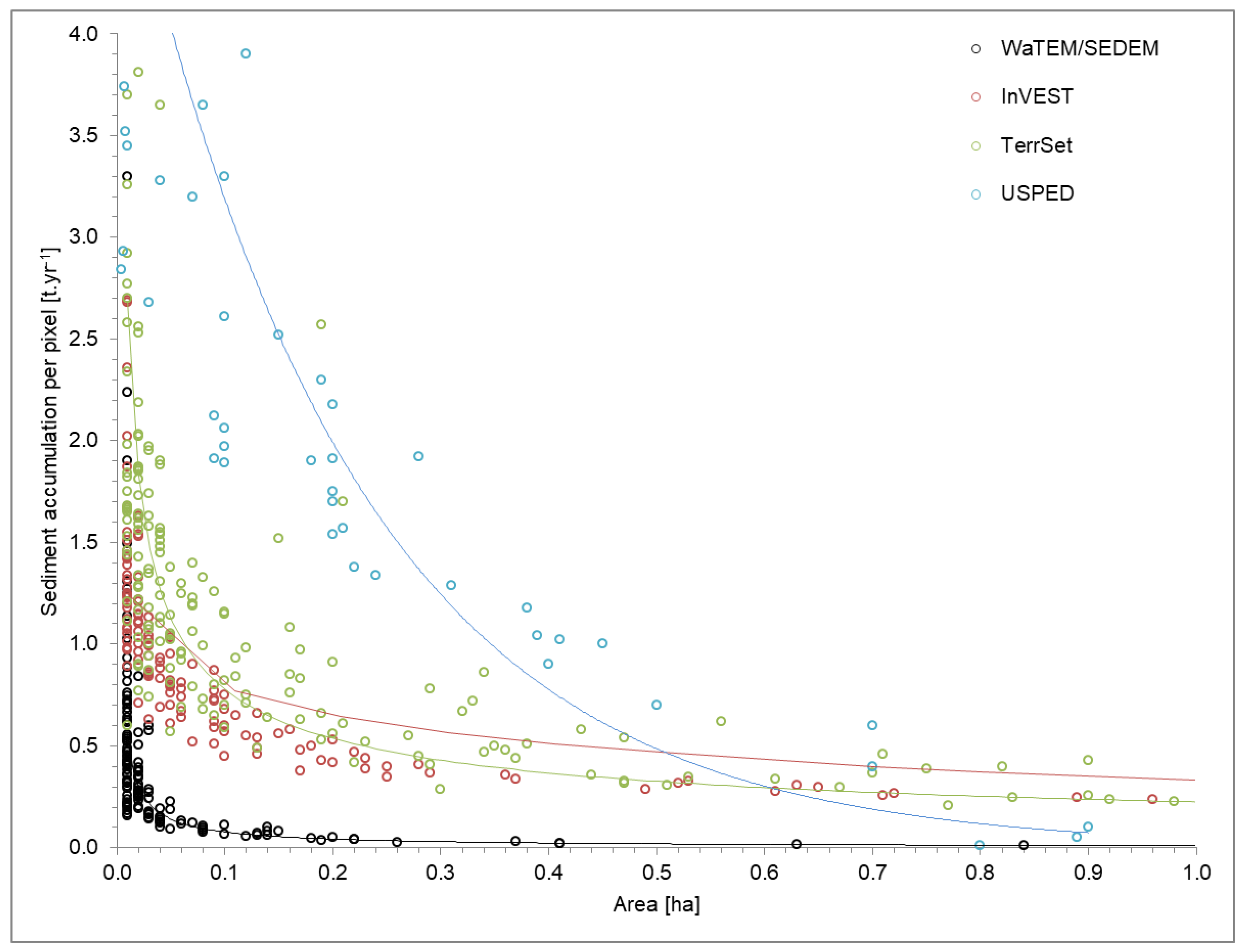
3.2. Analysis of Sediment Accumulation as a Consequence of Soil Loss by Water Erosion
4. Discussion and Conclusions
Author Contributions
Funding
Acknowledgments
Conflicts of Interest
References
- Pimentel, D. Soil erosion: A food and environmental threat. Environ. Dev. Sustain. 2006, 8, 119–137. [Google Scholar] [CrossRef]
- Kibblewhite, M.G.; Miko, L.; Montanarella, L. Legal frameworks for soil protection: Current development and technical information requirements. Curr. Opin. Environ. Sustain. 2012, 4, 573–577. [Google Scholar] [CrossRef]
- Communication from the Commission to the Council, the European Parliament, the European Economic and Social Committee and the Committee of the Regions—Thematic Strategy for Soil Protection. Brussels 2006. Available online: https://eur-lex.europa.eu/legal-content/EN/TXT/?uri=CELEX:52006DC0231 (accessed on 17 November 2018).
- Panagos, P.; Van Liedekerke, M.; Jones, A.; Montanarella, L. European Soil Data Centre (ESDAC): Response to European policy support and public data requirements. Land Use Policy 2012, 29, 329–338. [Google Scholar] [CrossRef]
- Morgan, R.P.C.; Quinton, J.N. Erosion modeling. In Landscape Erosion and Evolution Modeling; Springer: Boston, MA, USA, 2001; pp. 117–143. [Google Scholar]
- Nunes, J.P.; Seixas, J.; Pacheco, N.R. Vulnerability of water resources, vegetation productivity and soil erosion to climate change in Mediterranean watersheds. Hydrol. Process. Int. J. 2008, 22, 3115–3134. [Google Scholar] [CrossRef]
- Lorencová, E.; Frélichová, J.; Nelson, E.; Vačkář, D. Past and future impacts of land use and climate change on agricultural ecosystem services in the Czech Republic. Land Use Policy 2013, 33, 183–194. [Google Scholar] [CrossRef]
- Panagos, P.; Borrelli, P.; Poesen, J.; Ballabio, C.; Lugato, E.; Meusburger, K.; Montanarella, L.; Alewell, C. The new assessment of soil loss by water erosion in Europe. Environ. Sci. Policy 2015, 54, 438–447. [Google Scholar] [CrossRef] [Green Version]
- Nearing, M.A.; Pruski, F.F.; O’Neal, M.R. Expected climate change impacts on soil erosion rates: A review. J. Soil Water Conserv. 2004, 59, 43–50. [Google Scholar]
- Pruski, F.F.; Nearing, M.A. Runoff and soil-loss responses to changes in precipitation: A computer simulation study. J. Soil Water Conserv. 2002, 57, 7–16. [Google Scholar]
- De Vente, J.; Poesen, J.; Verstraeten, G.; Van Rompaey, A.; Govers, G. Spatially distributed modelling of soil erosion and sediment yield at regional scales in Spain. Glob. Planet. Chang. 2008, 60, 393–415. [Google Scholar] [CrossRef] [Green Version]
- Verstraeten, G.; Poesen, J. The nature of small-scale flooding, muddy floods and retention pond sedimentation in central Belgium. Geomorphology 1999, 29, 275–292. [Google Scholar] [CrossRef]
- Montgomery, D.R. Soil erosion and agricultural sustainability. Proc. Natl. Acad. Sci. USA 2007, 104, 13268–13272. [Google Scholar] [CrossRef] [PubMed] [Green Version]
- Wischmeier, W.H.; Smith, D.D. Predicting Rainfall Erosion Losses—A Guide to Conservation Planning; Science and Education Administration, USDA: Hyattsville, MD, USA, 1978; 62p.
- Renard, K.G.; Foster, G.R.; Weesies, G.A.; McCool, D.K.; Yoder, D.C. Predicting Soil Erosion by Water: A Guide to Conservation Planning with the Revised Universal Soil Loss Equation (RUSLE); United States Department of Agriculture: Washington, DC, USA, 1997.
- Guerra, C.A.; Maes, J.; Geijzendorffer, I.; Metzger, M.J. An assessment of soil erosion prevention by vegetation in Mediterranean Europe: Current trends of ecosystem service provision. Ecol. Indic. 2016, 60, 213–222. [Google Scholar] [CrossRef] [Green Version]
- Grimm, M.; Jones, R.J.; Rusco, E.; Montanarella, L. Soil erosion risk in Italy: A revised USLE approach. Eur. Soil Bureau Res. Rep. 2003, 11, 23. [Google Scholar]
- Van Rompaey, A.; Bazzoffi, P.; Jones, R.J.; Montanarella, L. Modeling sediment yields in Italian catchments. Geomorphology 2005, 65, 157–169. [Google Scholar] [CrossRef] [Green Version]
- Kouli, M.; Soupios, P.; Vallianatos, F. Soil erosion prediction using the revised universal soil loss equation (RUSLE) in a GIS framework, Chania, Northwestern Crete, Greece. Environ. Geol. 2009, 57, 483–497. [Google Scholar] [CrossRef]
- García-Ruiz, J.M. The effects of land uses on soil erosion in Spain: A review. Catena 2010, 81, 1–11. [Google Scholar] [CrossRef]
- Hallouz, F.; Meddi, M.; Mahé, G.; Toumi, S.; Rahmani, S.E.A. Erosion, Suspended Sediment Transport and Sedimentation on the Wadi Mina at the Sidi M’Hamed Ben Aouda Dam, Algeria. Water 2018, 10, 895. [Google Scholar] [CrossRef]
- Boardman, J.; Poesen, J. Soil erosion in Europe: Major processes, causes and consequences. Soil Erosion Eur. 2006, 4, 477–487. [Google Scholar]
- Scholz, G.; Quinton, J.N.; Strauss, P. Soil erosion from sugar beet in Central Europe in response to climate change induced seasonal precipitation variations. Catena 2008, 72, 91–105. [Google Scholar] [CrossRef]
- Mullan, D. Soil erosion under the impacts of future climate change: Assessing the statistical significance of future changes and the potential on-site and off-site problems. Catena 2013, 109, 234–246. [Google Scholar] [CrossRef]
- Jones, R.J.; Spoor, G.; Thomasson, A.J. Vulnerability of subsoils in Europe to compaction: A preliminary analysis. Soil Tillage Res. 2003, 73, 131–143. [Google Scholar] [CrossRef]
- Lieskovský, J.; Kenderessy, P. Modelling the effect of vegetation cover and different tillage practices on soil erosion in vineyards: A case study in Vráble (Slovakia) using WATEM/SEDEM. Land Degrad. Dev. 2014, 25, 288–296. [Google Scholar] [CrossRef]
- Novotný, I. Příručka Ochrany Proti Vodní Erozi; Ministerstvo Zemědělství: Praha, Czech Republic, 2014; 73p. (In Czech)
- Novotný, I. Příručka Ochrany Proti Erozi Zemědělské Půdy; Ministerstvo Zemědělství a Výzkumný ÚSTAV MELIOrací a Ochrany Půdy, v.v.i.: Praha, Czech Republic, 2017; 86p. (In Czech)
- Dostál, T.; Krása, J.; Váška, J.; Vrána, K. The map of soil erosion hazard and sediment transport in scale of the Czech Republic. Vodní Hospodářství 2002, 52, 46–48. (In Czech) [Google Scholar]
- Krása, J.; Dostál, T.; Vrána, K.; Plocek, J. Predicting spatial patterns of sediment delivery and impacts of land-use scenarios on sediment transport in Czech catchments. Land Degrad. Dev. 2010, 21, 367–375. [Google Scholar] [CrossRef]
- Van Rompaey, A.; Krása, J.; Dostál, T. Modelling the impact of land cover changes in the Czech Republic on sediment delivery. Land Use Policy 2007, 24, 576–583. [Google Scholar] [CrossRef]
- Konečná, J.; Karásek, P.; Fučík, P.; Podhrázská, J.; Pochop, M.; Ryšavý, S.; Hanák, R. Integration of Soil and Water Conservation Measures in an Intensively Cultivated Watershed – A Case Study of Jihlava River Basin (Czech Republic). Europ. Countrys. 2017, 1, 17–28. [Google Scholar]
- Doležal, F.; Kvítek, T.; Soukup, M.; Kulhavý, Z.; Tippl, M. Czech highlands and peneplains and their hydrological role, with special regards to the Bohemo-Moravian Highland. IHP HWRP-Berichte 2004, 2, 41–56. [Google Scholar]
- Janeček, M. Ochrana Zemědělské Půdy Před Erozí. Metodika; Česká Zemědělská Univerzita, Fakulta Životního Prostředí: Praha, Czech Republic, 2012; 113p. (In Czech) [Google Scholar]
- Desmet, P.J.J.; Govers, G. A GIS procedure for automatically calculating the USLE LS factor on topographically complex landscape units. J. Soil Water Conserv. 1996, 51, 427–433. [Google Scholar]
- Natural Capital Project. Available online: https://www.naturalcapitalproject.org/ (accessed on 5 May 2018).
- Borselli, L.; Cassi, P.; Torri, D. Prolegomena to sediment and flow connectivity in the landscape: A GIS and field numerical assessment. Catena 2008, 75, 268–277. [Google Scholar] [CrossRef]
- Cavalli, M.; Trevisani, S.; Comiti, F.; Marchi, L. Geomorphometric assessment of spatial sediment connectivity in small Alpine catchments. Geomorphology 2013, 188, 31–41. [Google Scholar] [CrossRef]
- Lopez-Vicente, M.; Poesen, J.; Navas, A.; Gaspar, L. Predicting runoff and sediment connectivity and soil erosion by water for different land use scenarios in the Spanish Pre-Pyrenees. Catena 2013, 102, 62–73. [Google Scholar] [CrossRef] [Green Version]
- Sougnez, N.; Wesemael, B.; Van Vanacker, V. Low erosion rates measured for steep, sparsely vegetated catchments in southeast Spain. Catena 2011, 84, 1–11. [Google Scholar] [CrossRef]
- Mitášová, H.; Hofierka, J.; Zlocha, M.; Iverson, L.R. Modelling topographic potential for erosion and deposition using GIS. Int. J. Geogr. Inf. Syst. 1996, 10, 629–641. [Google Scholar] [Green Version]
- Warren, S.D.; Mitášová, H.; Hohmann, M.G.; Landsberger, S.; Iskander, F.Y.; Ruzycki, T.S.; Senseman, G.M. Validation of a 3-D enhancement of the Universal Soil Loss Equation for prediction of soil erosion and sediment deposition. Catena 2005, 64, 281–296. [Google Scholar] [CrossRef]
- Pistocchi, A.; Cassani, G.; Zani, O. Use of the USPED model for mapping soil erosion and managing best land conservation practices. In Proceedings of the1st International Congress on Environmental Modelling and Software, Lugano, Switzerland, 24–27 June 2002. [Google Scholar]
- Pelacani, S.; Märker, M.; Rodolfi, G. Simulation of soil erosion and deposition in a changing land use: A modelling approach to implement the support practice factor. Geomorphology 2008, 99, 329–340. [Google Scholar] [CrossRef]
- Dotterweich, M.; Stankoviansky, M.; Minár, J.; Koco, Š.; Papčo, P. Human induced soil erosion and gully system development in the Late Holocene and future perspectives on landscape evolution: The Myjava Hill Land, Slovakia. Geomorphology 2013, 201, 227–245. [Google Scholar] [CrossRef]
- Bek, S.; Chuman, T.; Šefrna, L. The Usability of Contours in Erosion Modelling: A Case Study on ZABAGED, Czech Republic. Acta Universitatis Carolinae 2008, 1–2, 77–86. [Google Scholar]
- Vysloužilová, B.; Kliment, Z. Modelování erozních a sedimentačních procesů v malém povodí. Geografie 2012, 2, 170–191. (In Czech) [Google Scholar]
- CLARK LABS. Available online: https://clarklabs.org/about/ (accessed on 12 May 2018).
- Verstraeten, G.; Van Oost, K.; Van Rompaey, A.; Poesen, J.; Govers, G. Evaluating an integrated approach to catchment management to reduce soil loss and sediment pollution through modelling. Soil Use Manag. 2002, 18, 386–394. [Google Scholar] [CrossRef]
- WaTEM/SEDEM Homepage. Available online: http://geo.kuleuven.be/geography/modelling/erosion/watemsedem/index.htm (accessed on 5 May 2018).
- Hamel, P.; Falinski, K.; Sharp, R.; Auerbach, D.A.; Sánchez-Canales, M.; Dennedy-Frank, P.J. Sediment delivery modeling in practice: Comparing the effects of watershed characteristics and data resolution across hydroclimatic regions. Sci. Total Environ. 2017, 580, 1381–1388. [Google Scholar] [CrossRef] [PubMed]
- Notebaert, B.; Vaes, B.; Verstraeten, G.; Govers, G. WaTEM/SEDEM Version 2006 Manual; KU Leuven, Physical and Regional Geography Research Group: Leuven, Belgium, 2006. [Google Scholar]
- Bezak, N.; Rusjan, S.; Petan, S.; Sodnik, J.; Mikoš, M. Estimation of soil loss by the WaTEM/SEDEM model using an automatic parameter estimation procedure. Environ. Earth Sci. 2015, 74, 5245–5261. [Google Scholar] [CrossRef]
- Krása, J. Hodnocení Erozních Procesů Ve Velkých Povodních za Podpory GIS. Dizertační Práce; České Vysoké Učení Technické v Praze, Fakulta Stavební, Katedra Hydromeliorací a Krajinného Inženýrství: Praha, Czech Republic, 2004; 176p. (In Czech) [Google Scholar]
- Wolock, D.M.; McCabe, G.J. Comparison of Single and Multiple Flow Direction Algorithms for Computing Topographic Parameters in TOPMODEL. Water Resour. Res. 1995, 5, 1315–1324. [Google Scholar] [CrossRef]
- Pechanec, V.; Mráz, A.; Benc, A.; Cudlín, P. Analysis of spatiotemporal variability of C-factor derived from remote sensing data. J. Appl. Remote Sens. 2018, 12, 016022. [Google Scholar] [CrossRef]
- Doležal, F.; Kulhavý, Z.; Kvítek, T.; Soukup, M.; Čmelík, P.; Fučík, P.; Novák, J.; Peterková, E.; Pilná, P.; Pražák, M.; et al. Hydrologický výzkum v malých zemědělských povodích. J. Hydrol. Hydromech. 2006, 54, 217–229. (In Czech) [Google Scholar]
- Fučík, P.; Kaplická, M.; Kvítek, T.; Peterková, J. Dynamics of Stream Water Quality during Snowmelt and Rainfall—Runoff Events in a Small Agricultural Catchment. Clean Soil Air Water 2012, 40, 154–163. [Google Scholar] [CrossRef]
- Pavlík, F.; Dumbrovský, M.; Podhrázská, J.; Konečná, J. The influence of water erosion processes on sediment and nutrient transport from a small agricultural catchment area. Acta Univ. Agric. Silvic. Mendel. Brun. 2012, 60, 155–165. [Google Scholar] [CrossRef]
- Pechanec, V.; Burian, J.; Kiliánová, H.; Němcová, Z. Geospatial analysis of the spatial conflicts of flood hazard in urban planning. Morav. Geogr. Rep. 2011, 19, 41–49. [Google Scholar]


| Average Annual Values | Average Terrain Slope (°) | Average Stream Slope (°) | |||
|---|---|---|---|---|---|
| Precipitation (mm) | Discharge in Closing Profile (m3 s−1) | Specific Outflow (l.s−1 km-2) | Air Temperature (°C) | ||
| 665.0 | 0.027 | 3.802 | 7.1 | 18.3 | 2.6 |
| Factor | Factor description | Used Values | Unit | Data Source |
|---|---|---|---|---|
| R | Rainfall erosivity factor | 40.00 | MJ ha−1 cm h−1 | Janeček et al. [34] |
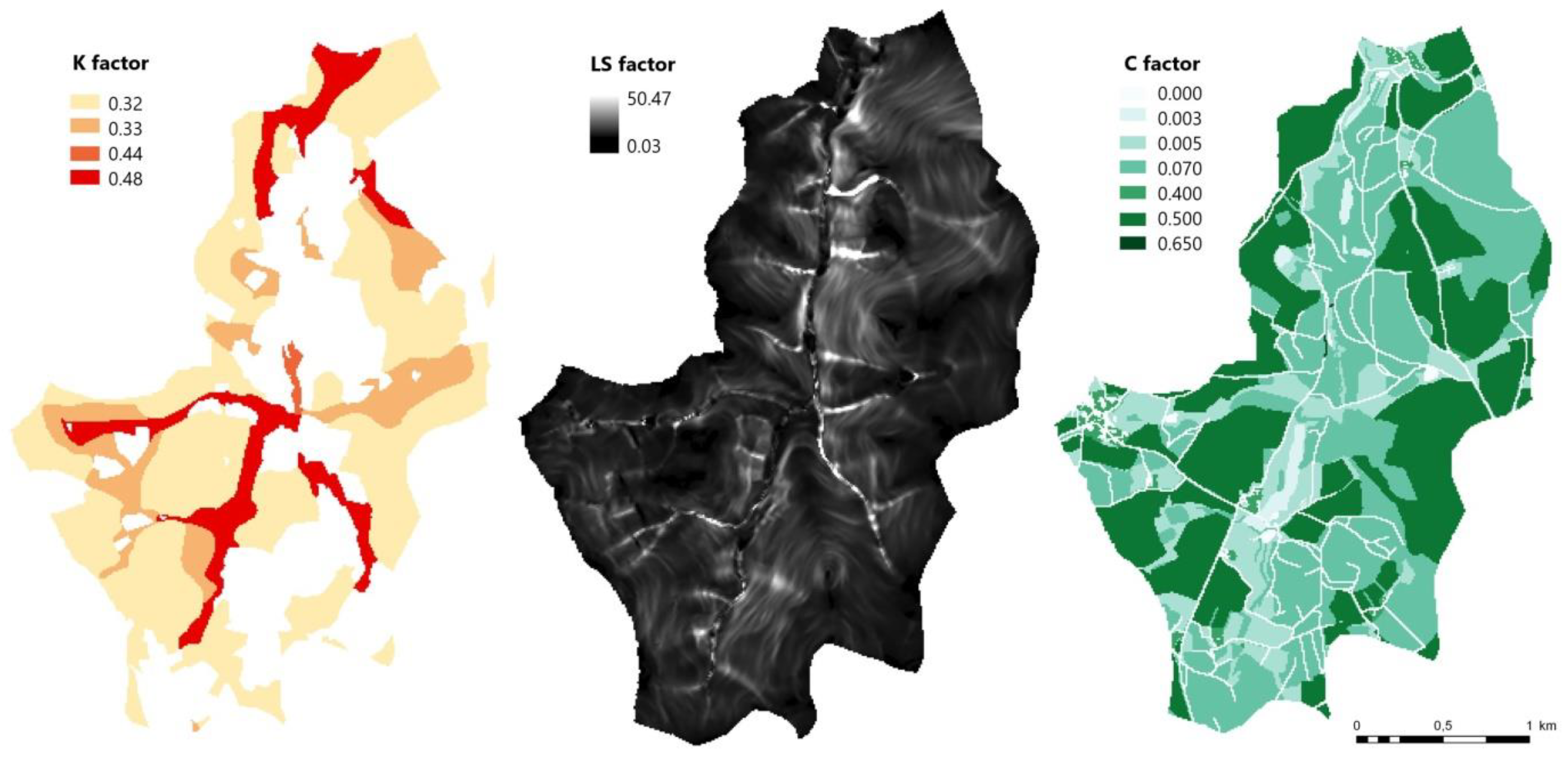
| K | Soil erodibility factor | 0.32–0.481 | t ha−1 | |
| LS | Topographic factor (slope length and steepness) | 0.03–50.471 | - | Own computation based on Desmet and Govers [35] |
| C | Cover and management factor | 0.00–0.651 | - | Janeček et al. [34] |
| P | Support practice factor | 1.00 | - |
| Model | InVEST | USPED | TerrSet | WaTEM/SEDEM | |
|---|---|---|---|---|---|
| Basic input parameters | DEM | Raster file | Raster file | Raster file | Raster file |
| R factor | Raster file | Numerical value | Raster file | Numerical value | |
| K factor | Raster file | Raster file | Raster file | Raster file or value | |
| LS factor | Numerical value | Raster file | Numerical value | Numerical value | |
| C factor | Numerical values (for each land-use category) | Raster file | Raster file | Raster file or value | |
| P factor | Numerical value | Numerical value | Raster file | Not included | |
| Other inputs (compulsory) | River basin layer (shapefile), Biophysical parameters, Land-use and land cover data, Flow accumulation threshold, Calibration parameters | Not included | Terrain properties to identify areas with similar erosion rates, SDR values | Watercourse layer (shapefile), Land-use and land cover data, Ptef, Parcel Connectivity Data, Calibration parameters | |
| Optional inputs | Information on drainage systems | Calibration parameters | No data value, Units used, Land fragmentation | Algorithm of LS factor computation, Retention ponds, Ploughing direction, Soil roughness, Units used | |
| Geodata format | Common raster file, Shapefile (.SHP), .CSV file (biophysical parameters only) | Common raster file | Idrisi file (.RST) | Idrisi file (.RST) | |
| Model Used | InVEST | USPED | TerrSet | WaTEM/SEDEM |
|---|---|---|---|---|
| Total soil loss in the basin (t year−1) | 43.78 | 76.03 | 55.38 | 41.96 |
| Total area with soil loss (ha) | 349.38 | 186.2 | 354.77 | 305.10 |
| Average soil loss (t ha−1 year−1) | 0.062 | 0.107 | 0.078 | 0.059 |
| Model Used | InVEST | USPED | TerrSet | WaTEM/SEDEM |
|---|---|---|---|---|
| Total soil accumulation in the basin (t year−1) | 21.24 | 80.84 | 22.42 | 39.86 |
| Total area with accumulation (ha) | 320.58 | 123.87 | 93.10 | 46.65 |
| Average soil accumulation (t ha−1 year−1) | 0.030 | 0.114 | 0.032 | 0.056 |
| Model Used | InVEST | USPED | TerrSet | WaTEM/SEDEM |
|---|---|---|---|---|
| Data pre-processing requirements | ++ | - | + | -- |
| User-friendly interface | ++ | 0 | + | + |
| Claims for prior user experiences | + | ++ | - | - |
| Failure sensitivity (including the difficulty of error detecting) | + | + | - | - |
© 2019 by the authors. Licensee MDPI, Basel, Switzerland. This article is an open access article distributed under the terms and conditions of the Creative Commons Attribution (CC BY) license (http://creativecommons.org/licenses/by/4.0/).
Share and Cite
Jakubínský, J.; Pechanec, V.; Procházka, J.; Cudlín, P. Modelling of Soil Erosion and Accumulation in an Agricultural Landscape—A Comparison of Selected Approaches Applied at the Small Stream Basin Level in the Czech Republic. Water 2019, 11, 404. https://doi.org/10.3390/w11030404
Jakubínský J, Pechanec V, Procházka J, Cudlín P. Modelling of Soil Erosion and Accumulation in an Agricultural Landscape—A Comparison of Selected Approaches Applied at the Small Stream Basin Level in the Czech Republic. Water. 2019; 11(3):404. https://doi.org/10.3390/w11030404
Chicago/Turabian StyleJakubínský, Jiří, Vilém Pechanec, Jan Procházka, and Pavel Cudlín. 2019. "Modelling of Soil Erosion and Accumulation in an Agricultural Landscape—A Comparison of Selected Approaches Applied at the Small Stream Basin Level in the Czech Republic" Water 11, no. 3: 404. https://doi.org/10.3390/w11030404