Optimizing the Water Treatment Design and Management of the Artificial Lake with Water Quality Modeling and Surrogate-Based Approach

Abstract
:1. Introduction
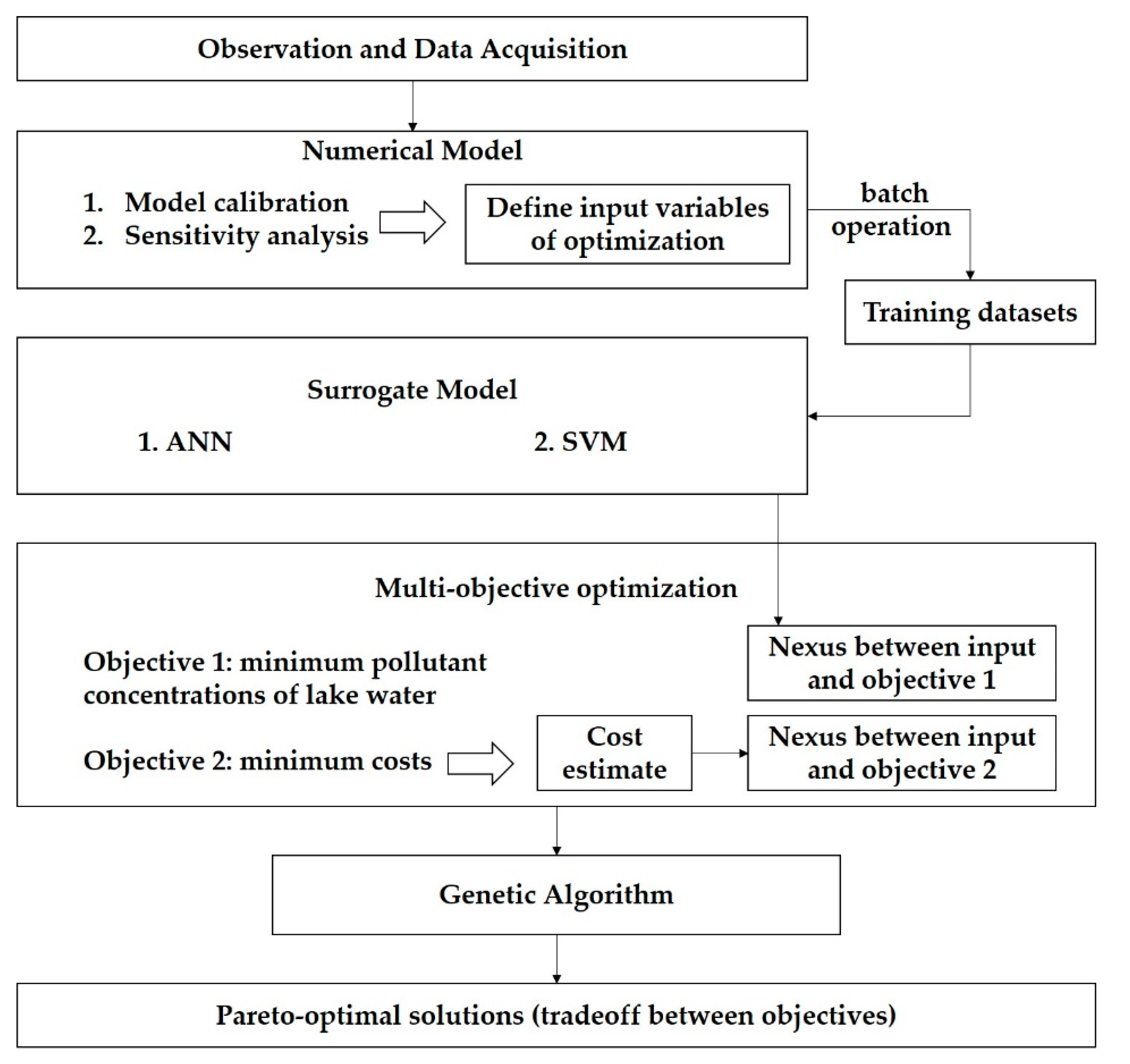
2. Modeling Roadmap
2.1. Introduction to MIKE21
2.2. ANN and SVM
3. Data and Methods
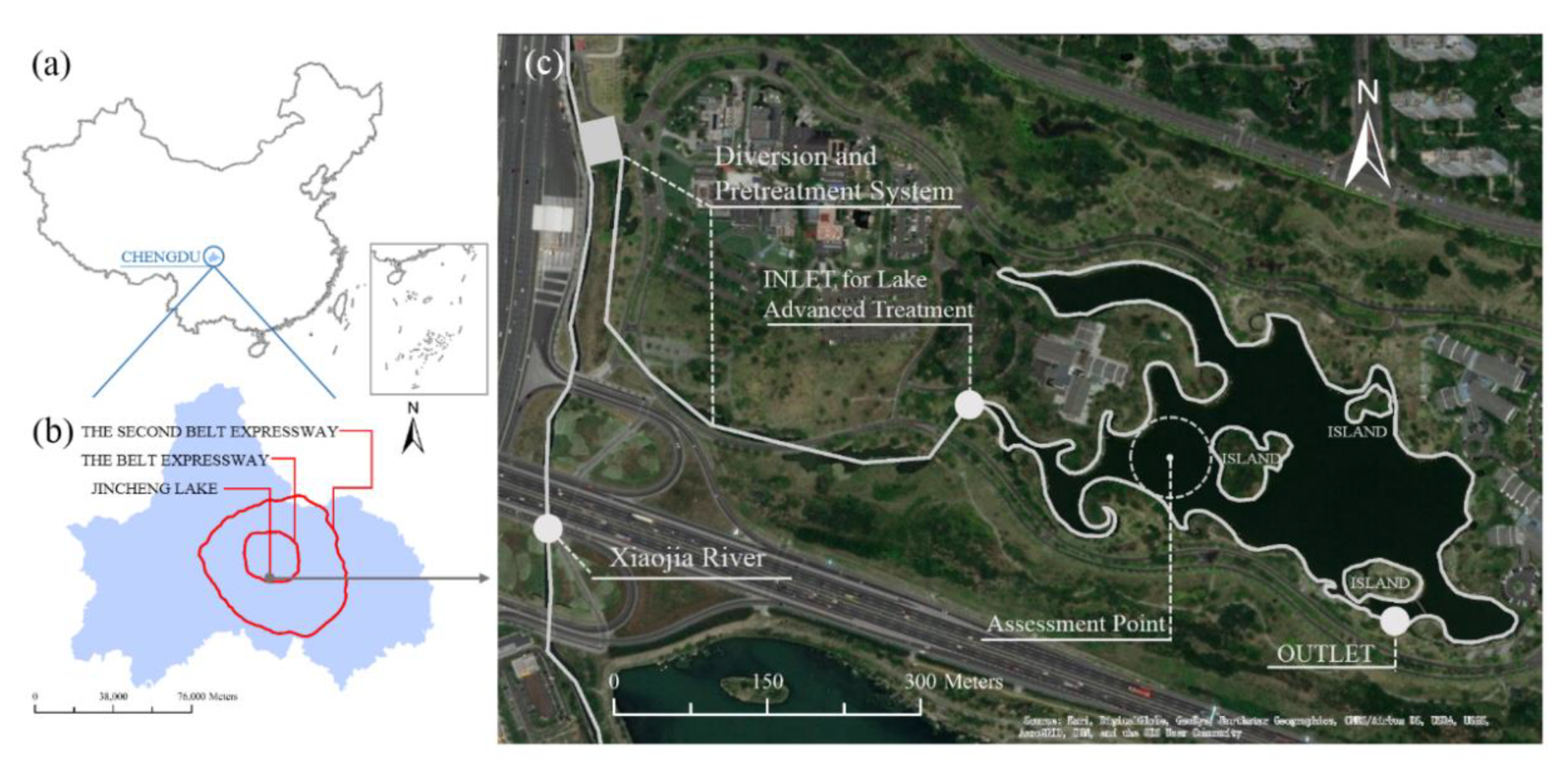
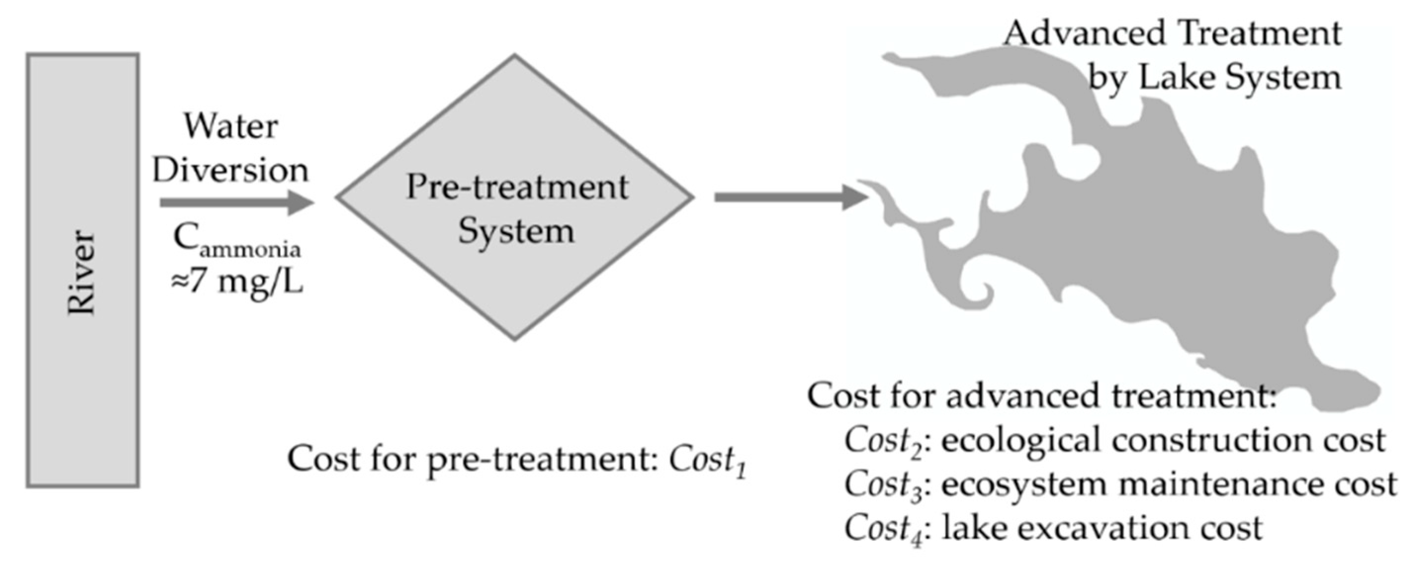
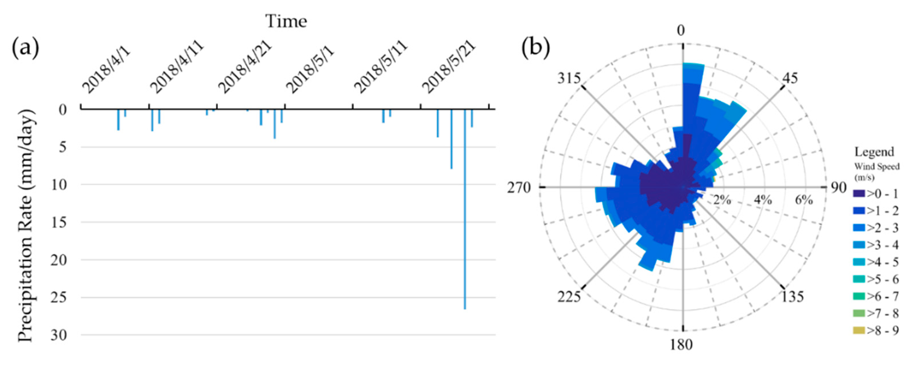
3.1. Study Site
3.2. Numerical Model Calibration and Sensitivity Analysis
3.3. Surrogate Model Training
3.4. Multi-Objective Optimization
4. Results and Discussion
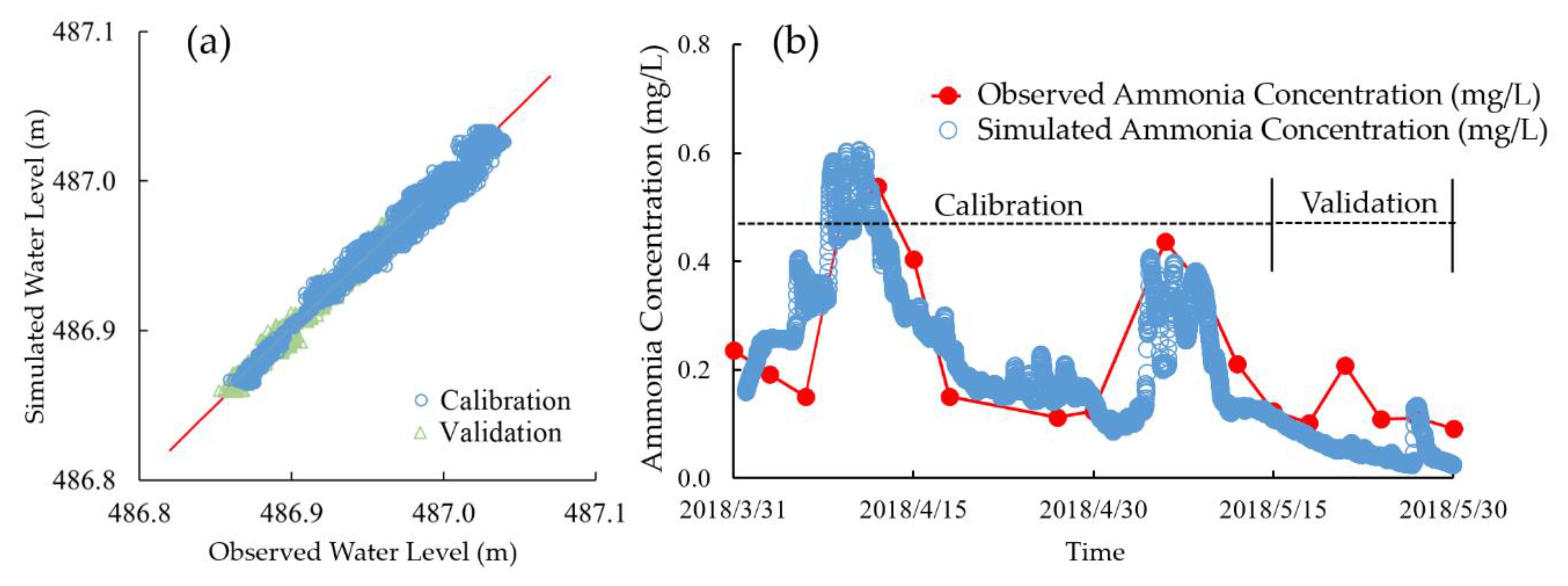
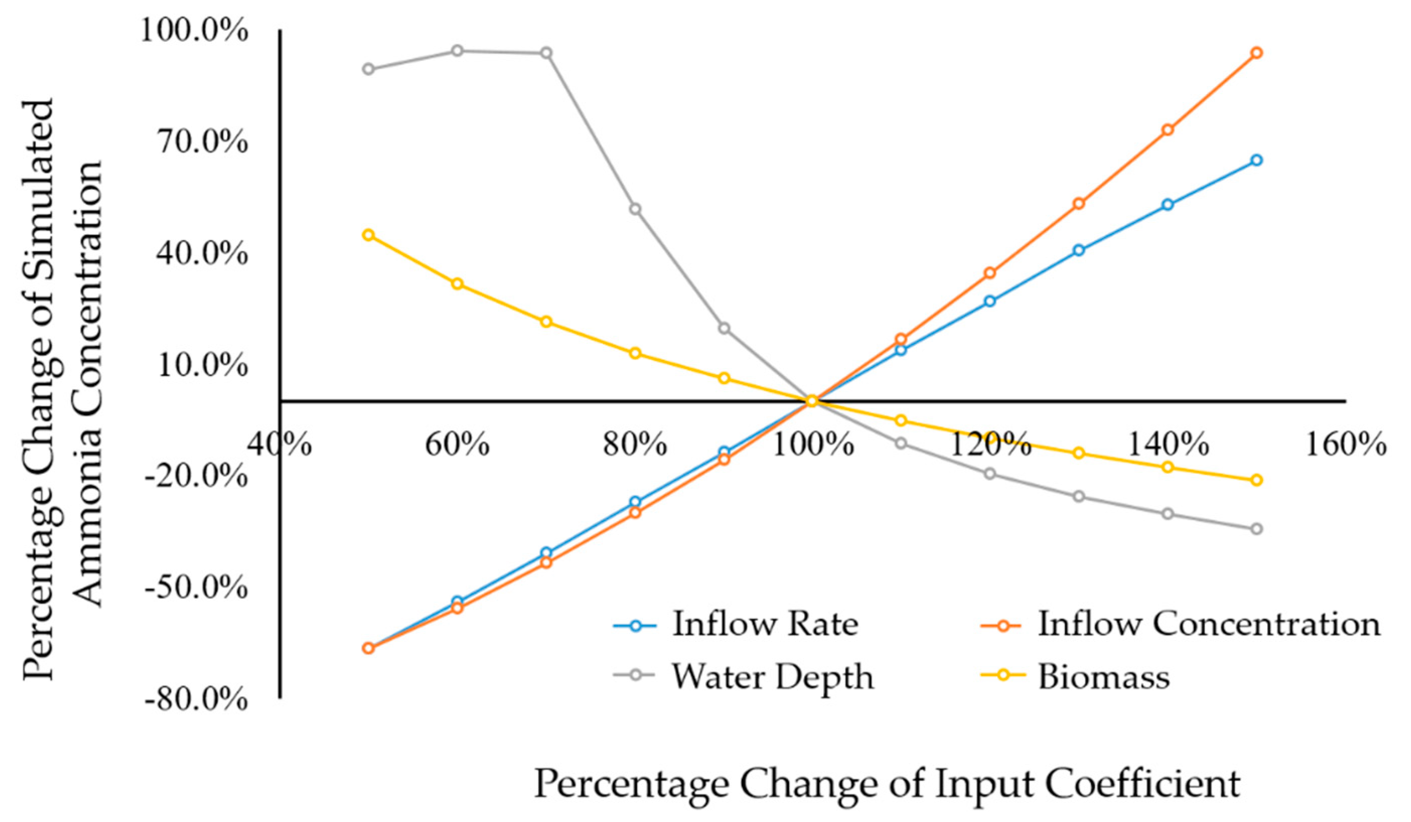
4.1. Model Calibration and Sensitivity Analysis
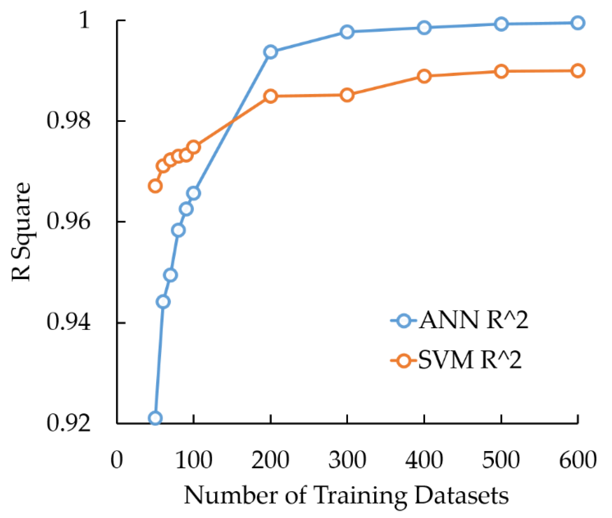
4.2. Surrogate Model Performances and Comparisons
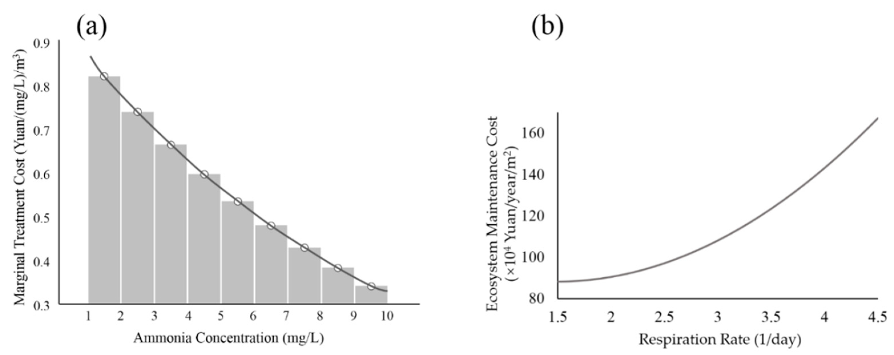
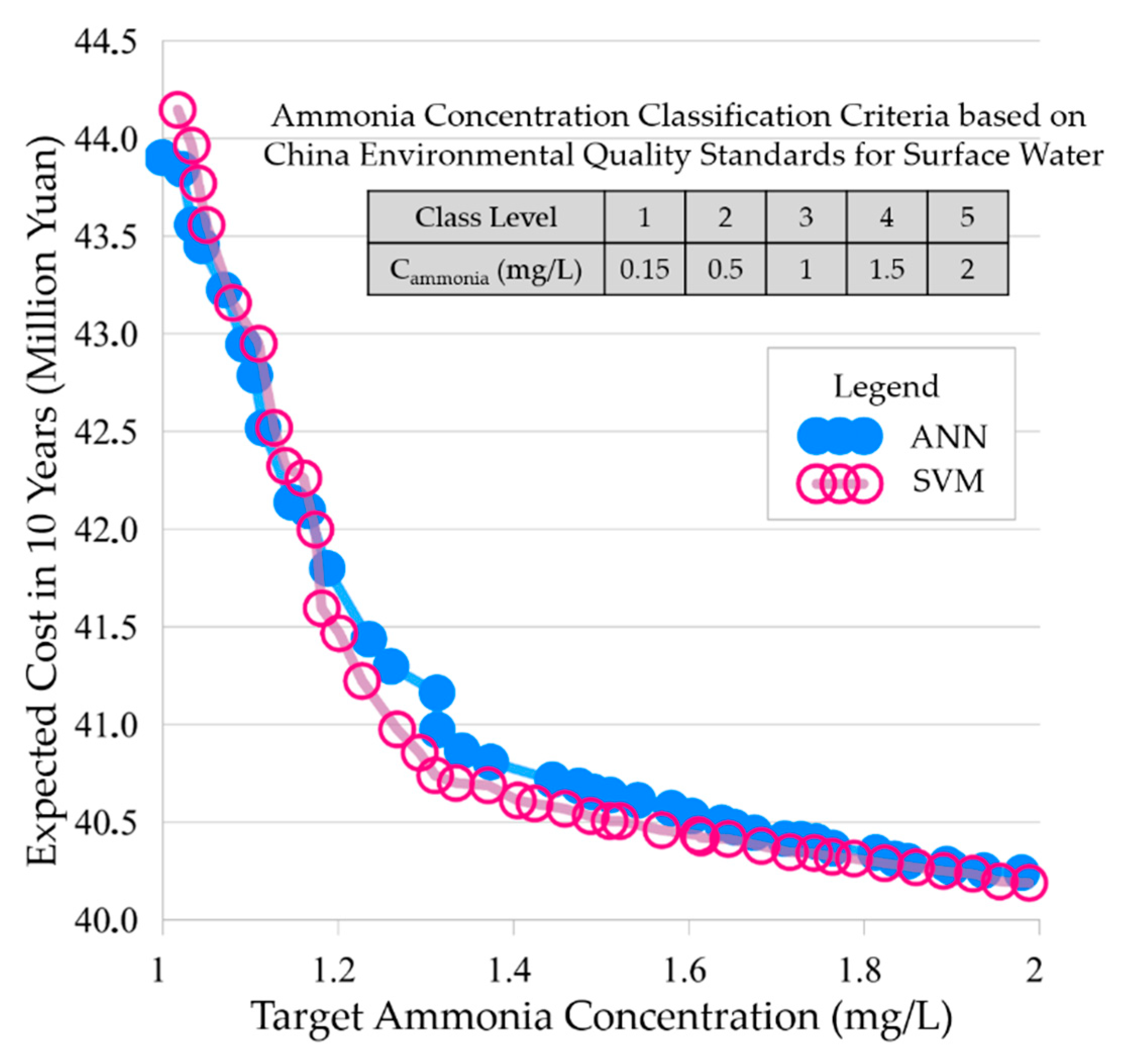
4.3. Multi-Objective Optimization of the Lake Design and Operation
5. Conclusions
Author Contributions
Funding
Conflicts of Interest
References
- Mortimer, C.H. Chemical Exchanges between Sediments and Water in the Great Lakes-speculations on Probable Regulatory Mechanisms. Limnol. Oceanogr. 1971, 16, 387–404. [Google Scholar] [CrossRef]
- Shutes, R.B.E. Artificial wetlands and water quality improvement. Environ. Int. 2001, 26, 441–447. [Google Scholar] [CrossRef]
- Moon, H.B.; Choi, M.; Yu, J.; Jung, R.H.; Choi, H.G. Contamination and potential sources of polybrominated diphenyl ethers (PBDEs) in water and sediment from the artificial Lake Shihwa, Korea. Chemosphere 2012, 88, 837–843. [Google Scholar] [CrossRef] [PubMed]
- Razavi, S.; Tolson, B.A.; Burn, D.H. Review of surrogate modeling in water resources. Water Resour. Res. 2012, 48, W07401. [Google Scholar] [CrossRef]
- Cai, X.; Zeng, R.; Kang, W.H.; Song, J.; Valocchi, A.J. Strategic planning for drought mitigation under climate change. J. Water Res. Plan. Manag. 2015, 141, 04015004. [Google Scholar] [CrossRef]
- Maier, H.R.; Kapelan, Z.; Kasprzyk, J.; Kollat, J.; Matott, L.S.; Cunha, M.C.; Marchi, A. Evolutionary algorithms and other metaheuristics in water resources: Current status, research challenges and future directions. Environ. Model. Softw. 2014, 62, 271–299. [Google Scholar] [CrossRef] [Green Version]
- Wang, C.; Duan, Q.; Gong, W.; Ye, A.; Di, Z.; Miao, C. An evaluation of adaptive surrogate modeling based optimization with two benchmark problems. Environ. Model. Softw. 2014, 60, 167–179. [Google Scholar] [CrossRef] [Green Version]
- Malekmohamadi, I.; Bazargan-Lari, M.R.; Kerachian, R.; Nikoo, M.R.; Fallahnia, M. Evaluating the efficacy of SVMs, BNs, ANNs and ANFIS in wave height prediction. Ocean Eng. 2011, 38, 487–497. [Google Scholar] [CrossRef]
- ASCE Task Committe. Artificial neural networks in hydrology. I: Preliminary concepts. J. Hydrol. Eng. 2000, 5, 115–123. [Google Scholar] [CrossRef]
- ASCE Task Committe. Artificial neural networks in hydrology. II: Hydrologic applications. J. Hydrol. Eng. 2000, 5, 124–137. [Google Scholar] [CrossRef]
- Ostad-Ali-Askari, K.; Shayannejad, M.; Ghorbanizadeh-Kharazi, H. Artificial neural network for modeling nitrate pollution of groundwater in marginal area of Zayandeh-rood River, Isfahan, Iran. KSCE J. Civ. Eng. 2017, 21, 134–140. [Google Scholar] [CrossRef]
- Sarkar, A.; Pandey, P. River water quality modelling using artificial neural network technique. Aquat. Procedia 2015, 4, 1070–1077. [Google Scholar] [CrossRef]
- Su, J.; Wang, X.; Zhao, S.; Chen, B.; Li, C.; Yang, Z. A structurally simplified hybrid model of genetic algorithm and support vector machine for prediction of chlorophyll a in reservoirs. Water 2015, 7, 1610–1627. [Google Scholar] [CrossRef]
- Gong, Y.; Wang, Z.; Xu, G.; Zhang, Z. A comparative study of groundwater level forecasting using data-driven models based on ensemble empirical mode decomposition. Water 2018, 10, 730. [Google Scholar] [CrossRef]
- Mohanty, S.; Jha, M.K.; Raul, S.; Panda, R.; Sudheer, K. Using artificial neural network approach for simultaneous forecasting of weekly groundwater levels at multiple sites. Water Resour. Manag. 2015, 29, 5521–5532. [Google Scholar] [CrossRef]
- Pan, C.C.; Chen, Y.W.; Chang, L.C.; Huang, C.W. Developing a Conjunctive Use Optimization Model for Allocating Surface and Subsurface Water in an Off-Stream Artificial Lake System. Water 2016, 8, 315. [Google Scholar] [CrossRef]
- Karahan, H.; Ayvaz, M.T. Simultaneous parameter identification of a heterogeneous aquifer system using artificial neural networks. Hydrogeol. J. 2008, 16, 817–827. [Google Scholar] [CrossRef]
- Cristianini, N.; Shawe-Taylor, J. An Introduction to Support Vector Machines; Cambridge University Press: Cambridge, UK, 2000. [Google Scholar]
- Liu, M.; Lu, J. Support vector machine—An alternative to artificial neuron network for water quality forecasting in an agricultural nonpoint source polluted river? Environ. Sci. Pollut. Res. 2014, 21, 11036–11053. [Google Scholar] [CrossRef] [PubMed]
- Lin, J.Y.; Cheng, C.T.; Chau, K.W. Using support vector machines for long-term discharge prediction. Hydrol. Sci. J. 2006, 51, 599–612. [Google Scholar] [CrossRef] [Green Version]
- Khalil, A.; Almasri, M.N.; McKee, M.; Kaluarachchi, J.J. Applicability of statistical learning algorithms in groundwater quality modeling. Water Resour. Res. 2005, 41, W05010. [Google Scholar] [CrossRef]
- Asefa, T.; Kemblowski, M.; Lall, U.; Urroz, G. Support vector machines for nonlinear state space reconstruction: Application to the Great Salt Lake time series. Water Resour. Res. 2005, 41, W12422. [Google Scholar] [CrossRef]
- Granata, F.; Gargano, R.; Marinis, G. Support vector regression for rainfall-runoff modeling in urban drainage: A comparison with the EPA’s storm water management model. Water 2016, 8, 69. [Google Scholar] [CrossRef]
- Tsoukalas, I.; Makropoulos, C. Multiobjective optimisation on a budget: Exploring surrogate modelling for robust multi-reservoir rules generation under hydrological uncertainty. Environ. Model. Softw. 2015, 69, 396–413. [Google Scholar] [CrossRef]
- Galán-Martín, Á.; Vaskan, P.; Antón, A.; Esteller, L.J.; Guillén-Gosálbez, G. Multi-objective optimization of rainfed and irrigated agricultural areas considering production and environmental criteria: A case study of wheat production in Spain. J. Clean. Prod. 2017, 140, 816–830. [Google Scholar] [CrossRef]
- Makropoulos, C.; Butler, D. A multi-objective evolutionary programming approach to the ‘object location’ spatial analysis and optimisation problem within the urban water management domain. Civ. Eng. Environ. Syst. 2005, 22, 85–101. [Google Scholar] [CrossRef]
- Brockhoff, D.; Zitzler, E. Objective reduction in evolutionary multiobjective optimization: Theory and applications. Evol. Comput. 2009, 17, 135–166. [Google Scholar] [CrossRef] [PubMed]
- Warren, I.; Bach, H.K. MIKE 21: A modelling system for estuaries, coastal waters and seas. Environ. Model. Softw. 1992, 7, 229–240. [Google Scholar] [CrossRef]
- Iturrarán-Viveros, U.; Parra, J.O. Artificial Neural Networks applied to estimate permeability, porosity and intrinsic attenuation using seismic attributes and well-log data. J. Appl. Geophys. 2014, 107, 45–54. [Google Scholar] [CrossRef]
- Shawe-Taylor, J.; Bartlett, P.L.; Williamson, R.C.; Anthony, M. Structural risk minimization over data-dependent hierarchies. IEEE Trans. Inf. Theory 1998, 44, 1926–1940. [Google Scholar] [CrossRef] [Green Version]
- Yao, Y.; Huang, X.; Liu, J.; Zheng, C.; He, X.; Liu, C. Spatiotemporal variation of river temperature as a predictor of groundwater/surface-water interactions in an arid watershed in China. Hydrogeol. J. 2015, 23, 999–1007. [Google Scholar] [CrossRef]
- Stein, M. Large sample properties of simulations using Latin hypercube sampling. Technometrics 1987, 29, 143–151. [Google Scholar] [CrossRef]
- Stephens, D.; Gorissen, D.; Crombecq, K.; Dhaene, T. Surrogate based sensitivity analysis of process equipment. Appl. Math. Model. 2011, 35, 1676–1687. [Google Scholar] [CrossRef] [Green Version]
- Zhang, X.; Srinivasan, R.; Van Liew, M. Approximating SWAT Model Using Artificial Neural Network and Support Vector Machine. J. Am. Water Resour. Assoc. 2009, 45, 460–474. [Google Scholar] [CrossRef] [Green Version]
- Behzad, M.; Asghari, K.; Eazi, M.; Palhang, M. Generalization performance of support vector machines and neural networks in runoff modeling. Expert Syst. Appl. 2009, 36, 7624–7629. [Google Scholar] [CrossRef]
- China EPA. Environmental Quality Standards for Surface Water; National Environmental Protection Agency of China: Beijing, China, 2002. (In Chinese)


| Item | Value | Unit | Item | Value | Unit |
|---|---|---|---|---|---|
| No. of time steps | 43200 | - | Ammonia decay rate at 20 °C | 0.5 | day−1 |
| Time step interval | 120 | s | Recharge rate | 0.033 | m3/s |
| Simulation start date | 2018/4/1 0:00:00 | - | Recharge ammonia concentration | 0.58 | mg/L |
| Simulation end date | 2018/5/31 0:00:00 | - | Water depth at the assessment point | 1.95 | m |
| Smagorinsky eddy viscosity | 0.28 | - | Respiration rate of animals and plants | 0.5 | day−1 |
| Manning coefficient | 32 | m1/3/s | Max. oxygen production by photosynthesis | 0.7 | day−1 |
| The ration of ammonia released at BOD decay | 0.29 | gNH4/gBOD | Uptake of ammonia in bacteria | 0.02 | - |
| Uptake of ammonia in plants | 0.03 | - |
| The Ammonia Concentration of Upstream River Water (mg/L) | The Optimal Target Ammonia Concentration (million yuan) | The Fractional Costs of the Pre-Treatment System | The Ammonia Concentration of Upstream River Water (mg/L) | The Optimal Target Ammonia Concentration (million yuan) | The Fractional Costs of the Pre-Treatment System |
|---|---|---|---|---|---|
| 4 | 21.9 | 28% | 8 | 46.5 | 54% |
| 5 | 28.8 | 39% | 9 | 51.4 | 57% |
| 6 | 35.2 | 45% | 10 | 55.7 | 59% |
| 7 | 41.2 | 50% |
© 2019 by the authors. Licensee MDPI, Basel, Switzerland. This article is an open access article distributed under the terms and conditions of the Creative Commons Attribution (CC BY) license (http://creativecommons.org/licenses/by/4.0/).
Share and Cite
Liu, C.; Hu, Y.; Yu, T.; Xu, Q.; Liu, C.; Li, X.; Shen, C. Optimizing the Water Treatment Design and Management of the Artificial Lake with Water Quality Modeling and Surrogate-Based Approach. Water 2019, 11, 391. https://doi.org/10.3390/w11020391
Liu C, Hu Y, Yu T, Xu Q, Liu C, Li X, Shen C. Optimizing the Water Treatment Design and Management of the Artificial Lake with Water Quality Modeling and Surrogate-Based Approach. Water. 2019; 11(2):391. https://doi.org/10.3390/w11020391
Chicago/Turabian StyleLiu, Chuankun, Yue Hu, Ting Yu, Qiang Xu, Chaoqing Liu, Xi Li, and Chao Shen. 2019. "Optimizing the Water Treatment Design and Management of the Artificial Lake with Water Quality Modeling and Surrogate-Based Approach" Water 11, no. 2: 391. https://doi.org/10.3390/w11020391