Article

Exploring the Influence Mechanism of Meteorological Conditions on the Concentration of Suspended Solids and Chlorophyll-a in Large Estuaries Based on MODIS Imagery

1
Department of Environmental Science and Engineering, Fudan University, Shanghai 200433, China
2
Shanghai Institute of Eco-Chongming (SIEC), Shanghai 200062, China
3
Big Data Institute for Carbon Emission and Environmental Pollution, Fudan University, Shanghai 200433, China
4
School of Environment, Nanjing Normal University, Nanjing 210023, China
5
Shanghai Investigation, Design & Research Institute Co., Ltd., Shanghai 200434, China
*
Authors to whom correspondence should be addressed.
Water 2019, 11(2), 375; https://doi.org/10.3390/w11020375
Submission received: 22 November 2018 / Revised: 14 February 2019 / Accepted: 16 February 2019 / Published: 21 February 2019
(This article belongs to the Section Water Quality and Contamination)

Abstract

:
In estuary areas, meteorological conditions have become unstable under the continuous effects of climate change, and the ecological backgrounds of such areas have strongly been influenced by anthropic activities. Consequently, the water quality of these areas is obviously affected. In this research, we identified periods of fluctuation of the general meteorological conditions in the Yangtze River Estuary using a wavelet analysis. Additionally, we performed a spatiotemporal evaluation of the water quality in the fluctuating period by using remote sensing modeling. Then, we explored how the fluctuating meteorological factors affect the distribution of total suspended solids (TSS) and chlorophyll-a (Chla) concentration. (1) The results show that from 2000 to 2015, temperature did not present significant fluctuations, while wind speed (WS) and precipitation (PR) presented the same fluctuation period from January 2012 to December 2012. (2) Based on the measured water sample data associated with Moderate Resolution Imaging Spectroradiometer (MODIS) imagery, we developed a water quality algorithm and depicted the TSS and Chla concentrations within the WS and PR fluctuating period. (3) We found that the TSS concentration decreased with distance from the shore, while the Chla concentration showed an initially decreasing trend followed by an increasing trend; moreover, these two water quality parameters presented different inter-annual variations. Then, we discussed the correlation between the changes in the TSS and Chla concentrations and the WS and PR variables. The contribution of this research is reflected in two aspects: 1. variations in water quality parameters over a wide range of water bodies can be evaluated based on MODIS data; 2. data from different time periods showed that the fluctuations of meteorological elements had different impacts on water bodies based on the distance from the shore. The results provide new insights for the management of estuary water environments.

1. Introduction

Estuaries are areas that interface with the ocean and represent destinations of watershed material; thus, they represent important natural regions that exchange many types of matter and energy between continents and oceans [1]. Consequently, such regions exert an extensive influence on the surrounding ecological environment. Unfortunately, recent studies have shown that water-quality problems in many estuaries are becoming serious due to the effects of human activities and climate change [2]. Industrialization and urbanization have negatively affected water quality, and the over-fertilization of agricultural activities and domestic wastes have led to an over-enrichment of nutrients in estuary water bodies [3,4]. Moreover, as the consequences of climate change become more visible, many researchers have recognized the increasing instability of weather conditions [5], which affect water and nutrient cycling, especially in vulnerable areas, such as estuaries.
The Yangtze River Estuary is located in eastern China, and as a nationally important sediment transport port, it plays an important role in social and economic development over the Yangtze River Delta [6]. According to long-term observation data from the Datong hydrological station, the average runoff of this river basin is greater than 9.05 × 10¹¹ m3 per year [7]. At the same time, the Yangtze River Estuary has also faced water-quality problems as observed in other estuaries around the world [8], especially under the rapid urbanization and industrialization process in the Yangtze River Delta, where anthropic activities are exacerbating water-quality problems [9]. Consequently, these water-quality problems have severely affected coastal reclamation and fishery production [10]. Therefore, monitoring the water-quality problems (especially those of sediment and eutrophication), identifying their spatiotemporal dynamics, and describing their influencing factors and mechanisms of interaction are important for water quality management in estuary areas.
Although field observation methods generate accurate measurements, they are time consuming and costly. Satellite remote sensing is a powerful monitoring tool for depicting spatial and temporal variations in water quality [11,12], especially for water-quality problems related to sedimentation and eutrophication, since these problems directly affect a water body’s spectral response in the visible and near infrared regions [13,14]. For water quality monitoring, total suspended solids (TSS) and chlorophyll-a (Chla) are widely used to control the sedimentation and eutrophication processes, respectively [15,16]. Specifically, TSS is a key variable for describing sediment dynamics [17] while Chla is an important proxy for phytoplankton biomass in aquatic ecosystems [18].
A number of satellite sensors have been used for water quality monitoring [19,20,21,22,23,24]. Several studies have proposed reliable algorithms for depicting water quality variables based on MODIS imagery [13,20,21,25]. Other recent studies have shown that water quality variables are obviously influenced by meteorological conditions [11,26]. Therefore, it is important to take the meteorological conditions into account in water-quality studies based on remote sensing methods.
Hence, the main aims of this study are as follows: (1) to identify the fluctuation periods of meteorological conditions during the study period, (2) to model the TSS and Chla concentrations in the Yangtze River Estuary based on MODIS images, and (3) to describe the influence of fluctuating meteorological conditions on water-quality variables.

2. Data and Methods

2.1. Data Pre-Processing

2.1.1. Collection of Water Samples and Laboratory Analysis

Water samples were collected from the water surface (approximately 50 cm) using Niskin bottles. All samples were placed in boxes and transported to the laboratory and filtered within 3 h to avoid the risk of degradation. The analysis of the TSS and Chla concentrations in all samples was completed within three days after collection.
From each water sample, 1 L was extracted to determine the TSS concentration, and sample filtration was performed with pre-weighed filters of 45-µm porosity and 47-mm diameter. The TSS concentration of every water sample was obtained as a function of the filtered water volume in mg/L by comparing the weight before and after filtration [27].
To analyze the content of Chla in the water samples, 1-L water samples were also extracted; these samples were filtered using 0.45-µm GF/F filters (Soochow Mary Precision Manufacture CO., LTD., Suzhou, China) at first and stored in the dark for 24 h at 4 °C. Subsequently, the samples were ground and centrifuged and then extracted with acetone. Then, the extinction rate of one drop of 1 mol/L hydrochloric acid before and after acidification was measured at 665 nm and 750 nm using a Shimadzu UV-2501 instrument (SHIMADZU Co.,LTD., Kyoto, Japan). Finally, the concentration of Chla was obtained according to the concentration calculation formula proposed by Chen [28]:
C C h l a = 27.9 V a c e t o n e [ ( E 665 E 750 ) ( A 665 A 750 ) ] / V s a m p l e
where Cchla is the concentration of chlorophyll-a (mg/m3); Vacetone is the volume of the volumetric solution of the extraction solution (mL); Vsample is the volume of filtered water (L); E665 and E750 are the extinction rates at 665 nm and 750 nm, respectively, before hydrochloric acid acidification; and A665 and A750 are the extinction rates at 665 nm and 750 nm, respectively, after hydrochloric acid acidification.

2.1.2. MODIS Satellite Data Pre-Processing
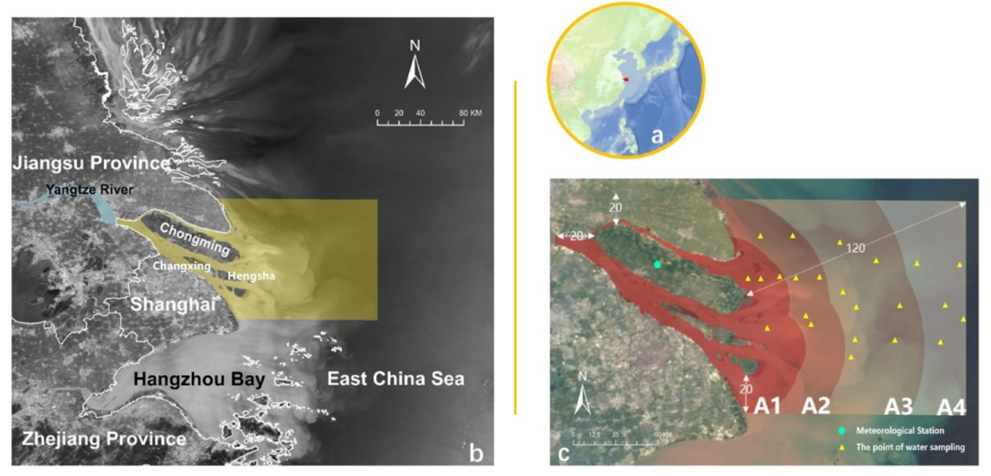
Considering the large area and the large variation in water quality, MODIS data are ideal because of their higher band resolution and shorter data period (approximately one-day intervals) [29]. MODIS/Terra 500-m resolution data were used in the data analysis because of the multi-band combination and spatial resolution. A total of five cloud-free MODIS/Terra 500-m resolution images from Level-1, which were captured from the Atmosphere Archive & Distribution System (LAADS) [30], were used to develop the MODIS-based evaluation model for TSS and Chla. Among the five remote sensing images, two of them had the same collection time as the water sample collection, and the difference between the other three and the time of the water sample collection was less than or equal to 4 days in order to avoid the influence of cloud occlusion and to ensure the synchronization between remote sensing data and measured data.
Cloud cover was extracted for each image using the MODIS cloud mask product MOD35. Then, considering the BOW-TIE phenomenon in the initial MODIS data [31], we calibrated the data using geometric correction based on the IDL (Interactive Data Language) and MRT (MODIS Reprojection Tool) software. The position accuracy of the corrected image was less than 0.5 pixels after processing. The radiometric calibration of data was carried out by offsets, scales, and other parameters in the original data. Then, referring to the relevant study, we used the Fast Line-of-sight Atmospheric Analysis of Spectral Hypercubes (FLAASH) atmospheric correction model to correct the data and reduce the radiation errors caused by atmospheric effects at the same time [32,33]. In addition, a constant amount of water vapor was considered for all pixels of the scene according to the atmospheric model, and depending on the water vapor content, different atmospheric models had different values. Here, the MODIS dates correspond to each sample collection event based on the Mid-Latitude Winter and Mid-Latitude Summer atmospheric model [34]. The rural aerosol model was selected according to the regional context, and the initial visibility was 25 km [35]. Finally, the elevation of the field was approximately 0 km, which was observed using Advanced Spaceborne Thermal Emission and Reflection Radiometer Global Digital Elevation Model (ASTER-GDEM) data.

2.2. Study Area

The Yangtze River Estuary is located in southeastern China (Figure 1a), and the spatial form is in the shape of a trumpet (Figure 1b). Water bodies in this area are mainly divided into three channels by Chongming Island in the north and ChangXing Island and HengSha Island in the south (Figure 1b) [6]. In this area, according to the observation data from hydrological stations, the annual average discharge and sediment transport are approximately 924 billion m2 and 486 million tons per year, respectively. Many observation results have shown that the spatial distribution of suspended sediment concentrations is not even in this area and ranges from 20 mg/L to 2500 mg/L [36,37]. According to the relevant research in this area, non-uniform wind, water waves, nutrient sources and other related natural and socio-economic conditions around this estuary area result in this uneven distribution of suspended sediment concentrations and eutrophication concentrations [6,38,39]. Consequently, other studies have pointed out that the uneven distribution patterns of water quality will impact the surrounding estuary ecosystem, especially the habitats related to bird and vegetation resources along Chongming Island [40].
The selected study area is shown in Figure 1b. The normalized difference water index (NDWI) [41] was used to identify the water body distribution around the Yangtze River Estuary from the 20-km buffer zone to the 120-m buffer zone from Chongming Island, Hengsha Island, and Changxing Island. Then, the rectangular region from the tangential line between the 20-km buffer on the north side and the 120-km buffer on the east side was considered the final research area based on a consideration of the trumpet shape and to facilitate future analyses. Water sample collection in this area was performed on two occasions: from 20 to 22 November 2012, and from 29 May to 1 June 2013. In total, 46 water samples were collected. We tried to keep the spatial distribution of the sampling sites fixed throughout the study area as shown in Figure 1c.

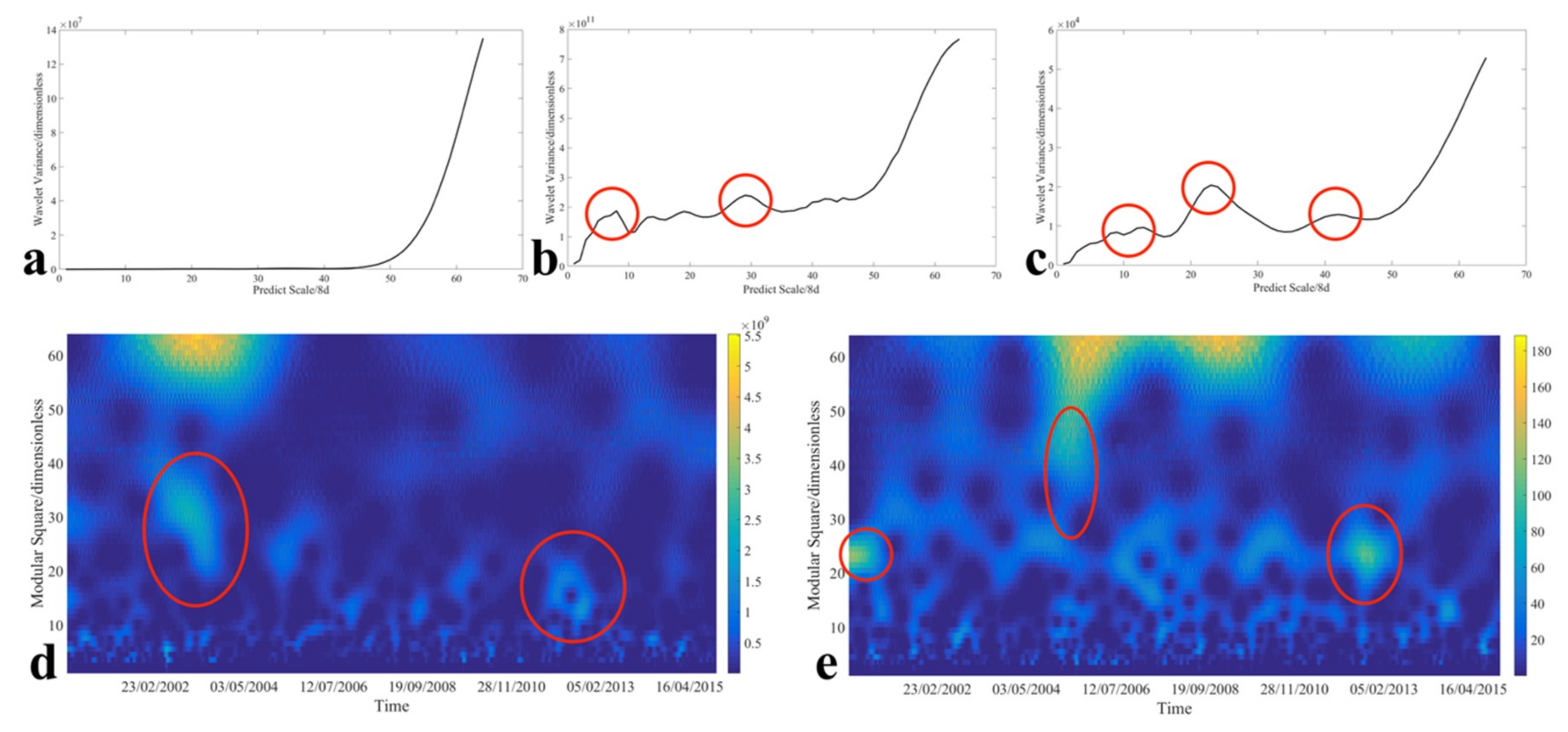
2.3. Meteorological Data Analysis

Referring to the relevant studies [42,43,44], temperature, precipitation (PR) and wind speed (WS) were selected. The daily temperature, PR and WS data from the Chongming meteorological station (shown in Figure 1c) were collected from the National Meteorological Information Center [45]. The time span of data is from 1 January 2000 to 31 December 2015. To simplify the calculation process and make the results more intuitive, the three meteorological variables were calculated over an average period of eight days. Then, these three variables in all eight-day periods were assessed for further analysis.
In addition, to identify the abnormal time periods for meteorological conditions, wavelet analysis was used in this study to describe the fluctuation and attenuation characteristics and mark the abnormal time period. Specifically, we used the continuous wavelet transform (CWT) method [46,47], and the formula of this method is as follows:
W f ( a ,   b ) = | a | 1 2 R f ( t ) ψ ¯ ( t b a ) d t
where W f ( a ,   b ) represents the wavelet transform coefficient, f(t) represents the signal or square integrable function, b represents the translation parameter, and ψ ¯ ( t b a ) represents the complex conjugate function of ψ ( t b a ) [48,49].
The variation of the wavelet (Var(a)) is as follows:
Var ( a ) = | W f ( a , b ) | 2 d b
This equation can be used to determine the relative intensity of the different mesoscale disturbances of the study period.

2.4. Model Development and Accuracy Evaluation

Before the model development, it is necessary to determine which band reflectance or band combination is most suitable for predicting the TSS and Chla. We used the Pearson correlation index to test the correlation relationship between the water quality and the band value [50].
Subsequently, to calculate and determine which model is most suitable for local water quality assessments, different studies have used different methods of measuring the accuracy of the model. In this study, the R2, mean absolute percentage error (MAPE), and root mean square error (RMSE) were used, and the formulas for calculating the MAPE and RMSE are as follows:
MAPE = 1 n i = 1 n | W Q m e a s i W Q p r e d i W Q m e a s i | × 100 %
R M S E = i = 1 n ( W Q m e a s i W Q p r e d i ) 2 n
where W Q m e a s i and W Q p r e d i represent the measured and predicted water quality concentrations for the i-th sample, respectively. The closer the MAPE and RMSE values are to 0, the better the prediction of the model. The prediction effect of the model is greater as the R2 value approaches 1.

3. Results

3.1. Meteorological Time Series

The results of the meteorological data analysis are shown in Figure 2. Among them, Figure 2a confirms that a significant fluctuation phenomenon did not occur for air temperature within the study period. In contrast, Figure 2b shows that PR fluctuated and presented a main fluctuation cycle on the 25–35 time scale and a second fluctuation cycle on the 8–10 time scale. In Figure 2c, the WS fluctuated on the 10–15, 20–30, and 40–50 time scales, with the main fluctuating cycle on the 20–30 time scale and the second fluctuating cycle on the 40–50 time scale. Then, to determine the specific time of the fluctuation cycle of PR and WS, the wavelet power spectrum corresponding to the PR and WS variables was obtained based on the CWT method. According to Figure 2d, the main fluctuation cycle of PR occurred within the 100–200th 8-day period and the 550–600th 8-day period of the study period. Figure 2e indicates that the main fluctuation cycle of WS appeared in the 0–50th 8-day period and the 550–600th 8-day period of the study period. These two variables both fluctuated during the 550–600th 8-day period, and this time period corresponds to the actual time from January 2012 to December 2012 as shown in Figure 2d,e. Therefore, this study chose the period from spring to the end of winter of 2012 as the research time period to explore the impact of exceptionally strong fluctuations of PR and WS on water quality.

3.2. Algorithm Development and Accuracy Evaluation

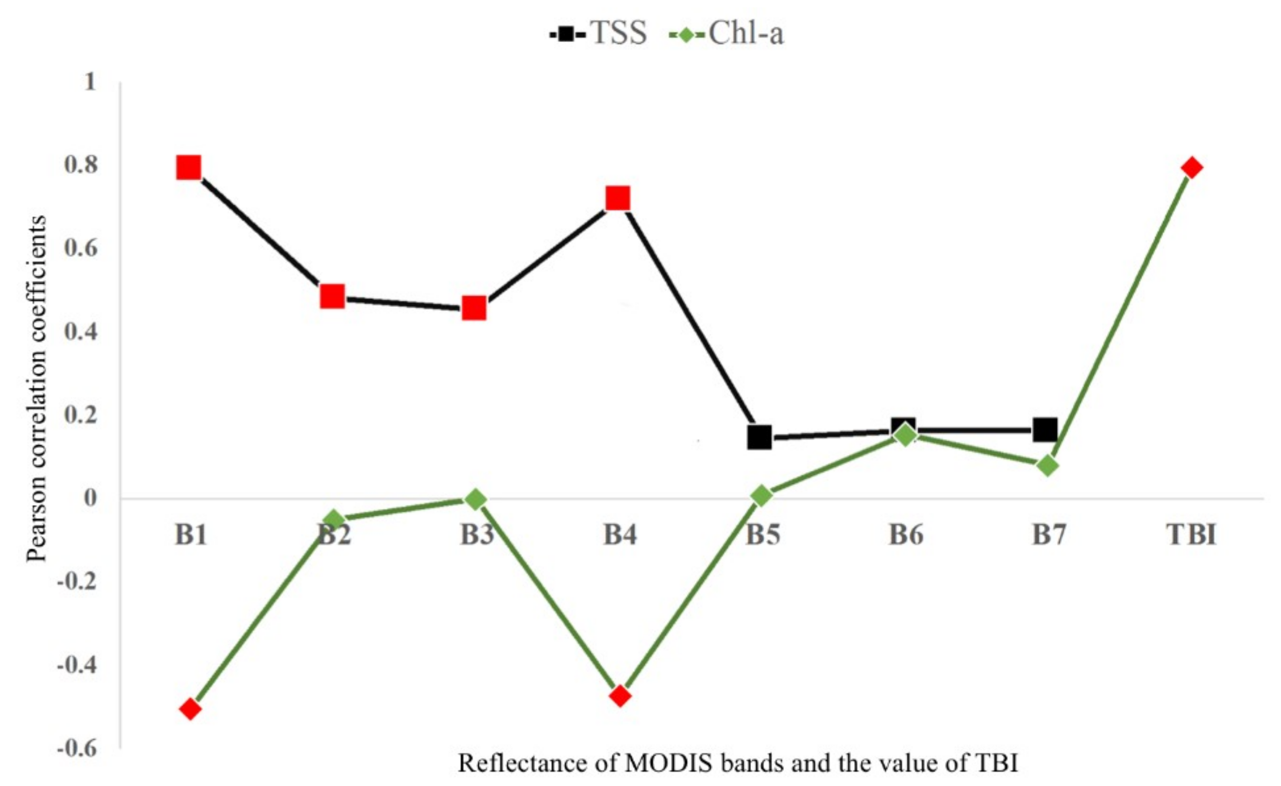
3.2.1. Band Selection for the Algorithm Development

Figure 3 shows the Pearson correlation results between the band values of MODIS data and the in situ TSS and Chla concentration measures. The relationship between TSS concentrations and single band data is high. High concentrations of suspended solids generally enhance the scattering value of each band and absorb a considerable amount of light [51], weakening the correlation between single band value anc Chla-concentrations [52].
According to these characteristics, we developed the model to evaluate TSS and Chla from a different point of view. Band 1 and band 4 were used to develop the TSS evaluation model because of the higher Pearson correlation values. Through the use of multiple linear regression models, we incorporated both band 1 and band 4 to build the TSS evaluation model. For the evaluation of Chla, many studies have been carried out using single-band numerical modelling [12,53]. Considering the need to reduce the effect of TSS on the Chla spectra, we chose the three-band index (TBI) to evaluate the concentration of Chla. Based on the feature of MODIS data, we selected the optimized TBI model from related research [54]. The calculation process of this model is as follows:
TBI = [ R 1 ( b 1 ) R 1 ( b 3 ) × R 1 ( b 4 ) ] × R ( b 2 )
where bi represents the i band of MODIS, and R(bi) represents the reflectivity of the i band. This method has been widely used in other studies under the condition of higher suspended solids concentration [55], especially in estuaries and other turbid water bodies [54,56,57,58]. We analyzed the correlation between the TBI and Chla measured data. The Pearson correlation index was 0.81, which indicated that this index could reduce the effect of high TSS concentrations on the Chla under the condition of high suspended solids concentration and improve the accuracy of the Chla evaluation model in the study area.

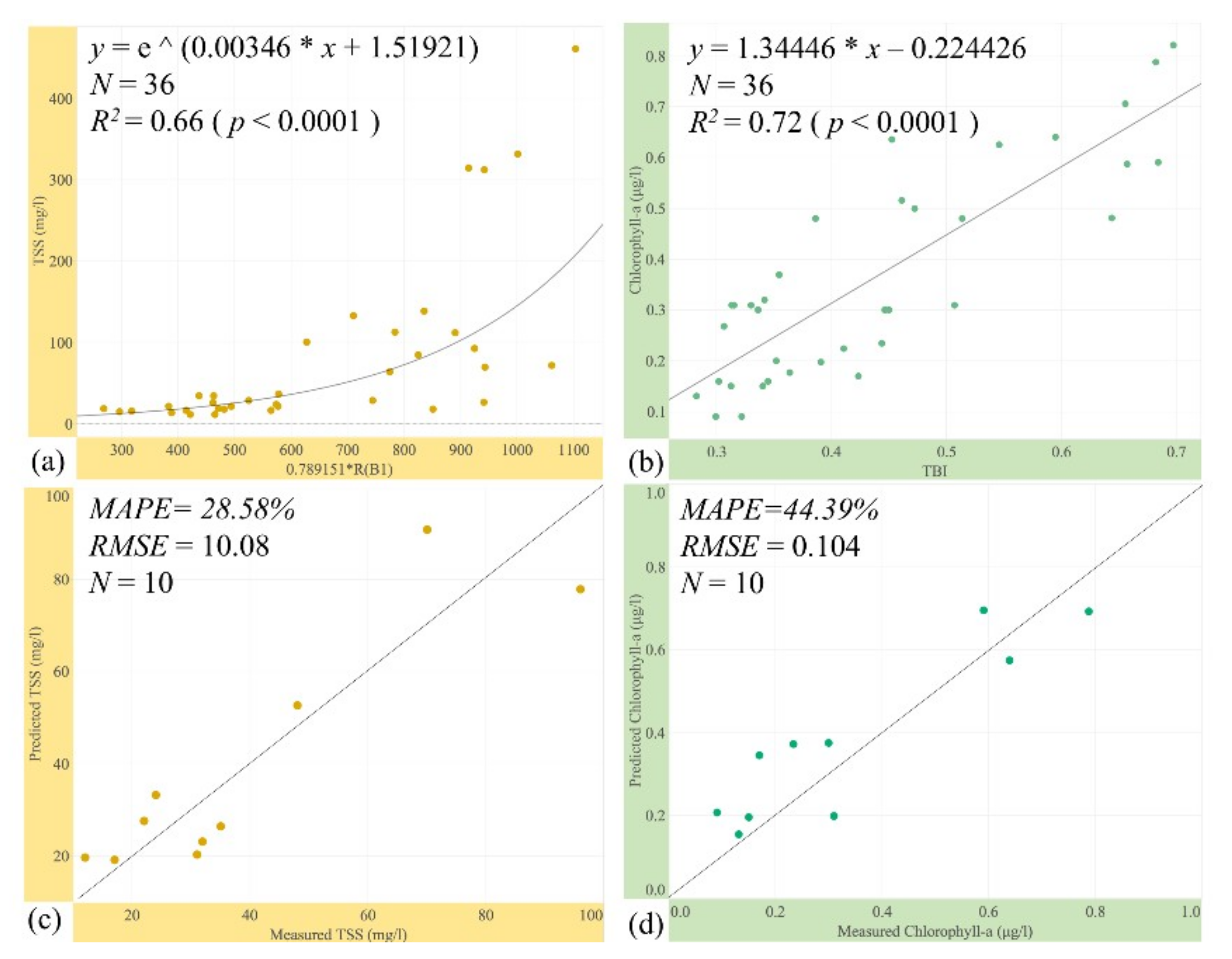
3.2.2. Algorithm Development

We developed the TSS and Chla evaluation algorithm model based on the in situ data and the MODIS band reflectance after correction. Specifically, all water sample databases were divided into two groups to develop the remote sensing algorithm models: one group was used to control the algorithm development (36 water samples, accounting for approximately 80% of all data) and the other water sample group (10 water samples, accounting for approximately 20% of all data) was used as an independent dataset to verify the accuracy of the algorithm. In addition, the previous section showed that the spectral properties of TSS and Chla are quite different. Therefore, two random groupings of all data were generated in aiming to evaluate the concentrations of TSS and Chla.
Based on the high correlation index (i.e., the index obtained by the multiple linear regression for TSS and by the TBI for Chla), linear, nonlinear and exponential correlations (linear, power low, exponential, quadratic, etc.) were used to analyze the relationship between the model results and the measured concentrations of TSS and Chla to determine which model had the best fit. Two models were finally developed:
C T S S = e ( 0.00346 × ( 0.78915 × R ( b 1 ) ) + 1.51921 )
C C h l a = 1.34446 × T B I 0.224426
CTSS and CChla represent the concentration of TSS and Chla, bi represents the i band of MODIS, and R(bi) represents the band reflectivity of bi. It is important to note that although band 4 had a high correlation with the TSS concentration, band 4 was not considered in the results of the TSS evaluation algorithm because in the multiple linear regression, the probability of the Student’s t test corresponding to band 4 was 0.15 >0.1; therefore, the regression analysis did not consider band 4. In Fábio’s study, only band 1 was considered when calculating the TSS concentration [12].
As shown in Figure 4, to demonstrate the accuracy of the model predictions, we evaluated the accuracy of each model and found that each evaluation index performed well. The MAPE and RMSE values of the TSS remote estimation model were 28.58% and 10.08, respectively (Figure 4c). The MAPE and RMSE values of the Chla remote estimation model were 44.39% and 0.104, respectively (Figure 4d). Although the accuracy of these algorithm results is limited, the evaluation results revealed, in consideration of the large study area, the data quasi-synchronization problem, and the RMSE value of these two models are less than the accuracy results from other studies in similar research areas [12,23,24]; therefore, we considered the accuracy of our model to adequately meet our requirements in depicting the water quality distribution in this large estuary area. Thus, MODIS data for other time periods can be input into these models to evaluate the concentrations of TSS and Chla across time scales.

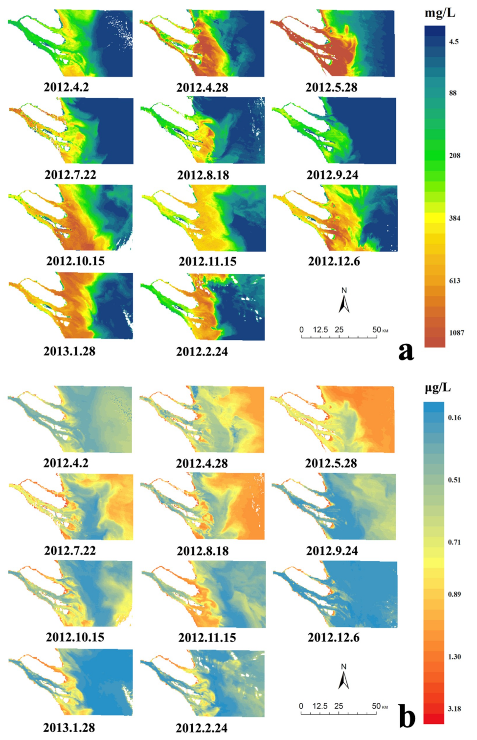
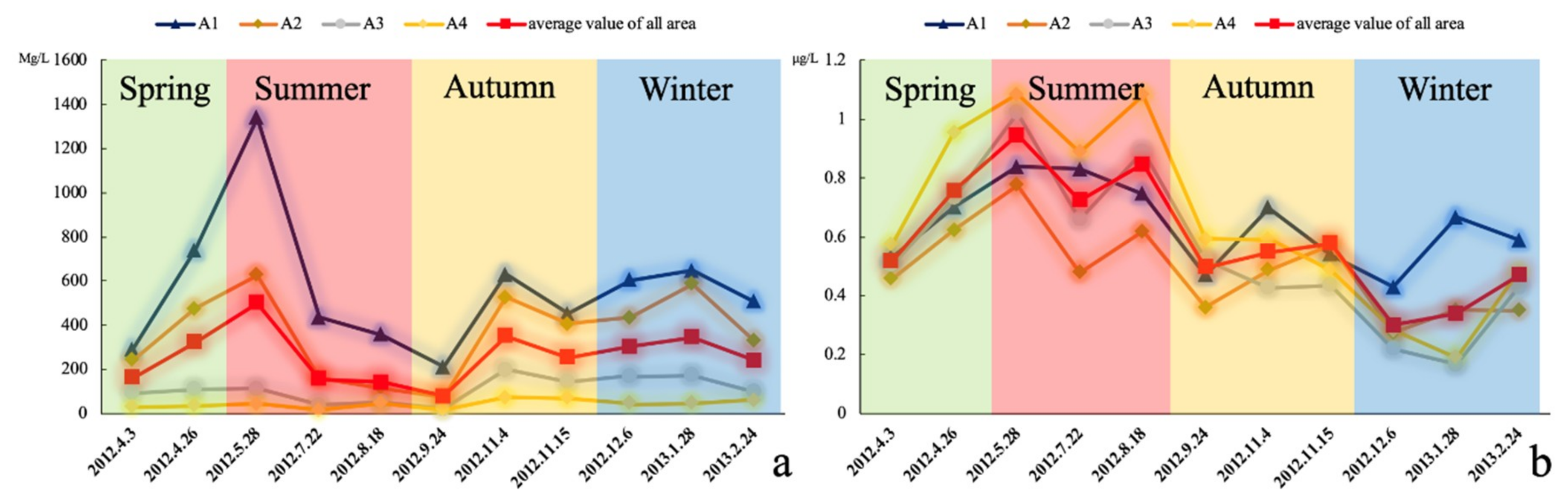
3.3. Spatiotemporal Variations

We obtained MODIS images with low cloud cover throughout the study area during the period from March 2012 to February 2013, when the PR and WS have the greatest fluctuations. All images (a total of 45 MODIS images) were then screened on the condition that the interval was greater than 15 days (a total of 11 images was finally selected), considering the distinct characteristics of the four seasons in the subtropical region: spring is from March to May, summer is from June to August, autumn is from September to November, and winter is from December to February of the next year. These selected images were then pre-processed.
Figure 5 intuitively reflects the changing trends of the TSS and Chla concentrations in different spaces and times, which is similar to other relevant evaluation results in this area [15,59]. Figure 6 shows the average concentration of the evaluation results of each region in each period.
Overall, as shown in Figure 5, there are obvious differences between the TSS and Chla concentration. The concentration of TSS ranged from 4.5 mg/L to 2039.01 mg/L, with a mean value of 259.89 mg/L, and the value decreased from the land to the sea. Seasonally, the mean values of winter and summer were significantly higher than those of spring and autumn, which is consistent with Wu’s study results [60]. Specifically, the high TSS concentration value was mainly located in the coastal areas in summer, while the TSS concentration values in winter were more scattered. The concentration of Chla showed an obvious band-gap distribution, in which the mean value of the area farther offshore (A4) was the highest (0.66 ± 0.29 μg/L) and the mean value of the middle region (A2) was the lowest (0.49 ± 0.14 μg/L). Seasonally, the average values in spring and summer were higher than that in winter, and the values were more dispersed in spring and summer than in winter.

4. Discussion

In this study, we selected the influence of three meteorological factors: (1) Temperature: the water surface temperature is directly related to the growth of aquatic plants and microorganisms in the water body [61,62]. (2) PR: a high level of PR increases the surface water flow into the estuary area, representing an important source for sediment and nutrient contents [62,63]. (3) WS: the WS not only affects the water surface flow and sediments but also affects the strength of the ocean currents near the estuary area [64,65].
The results of this study confirm the usefulness of MODIS data to evaluate water quality indicators in aquatic ecosystems [66,67].
In terms of model accuracy, the MAPE and RMSE values were relatively small for the model in this study, indicating that the results are better than those of other TSS and Chla evaluation studies based on MODIS data.
The use of remote sensing to evaluate the water quality is mainly based on the principle that the water spectral characteristics are affected by the material activity in the water body. Therefore, combining different bands can obtain more information about active substances in the water bodies. Considering that the spectral characteristics of Chla were affected by the high TSS concentration in the estuary, the single-band model was not satisfactory. Thus, we considered applying more complex band combinations to reduce the impact of TSS on the development of the Chla evaluation model.
Based on the results of spatiotemporal variations, we found that there are obvious differences in the amplitude of the seasonal variations in the different regions, which may be due to the different effects of PR and WS in the different regions. We further discuss the impact factors of different types of water quality.

4.1. Factors Affecting TSS concentration

First, we calculated the mean WS and accumulated PR over the 15 days before the corresponding date of each MODIS data point acquisition time. We used the Pearson correlation index to evaluate the correlation between the TSS mean value with the mean WS and cumulative PR values in the entire study area and four sub-regions. As shown in Table 1, a significant correlation was observed between the mean TSS concentration and the mean WS (Pearson correlation index = −0.67, p <0.05) and the accumulated PR (Pearson correlation index = −0.554, p <0.05) in the study area. A positive correlation was observed between the TSS concentration and PR (Pearson correlation index >0), although a negative correlation was observed between the TSS and WS (Pearson correlation index <0). These results were obtained for several reasons. 1. In addition to the large amount of sediment carried by the upper reaches of the Yangtze River, the inflow of peripheral runoff is also an important source of sediment, and the PR process will rapidly increase the sediment content in the suspended matter of rivers, and this content is transmitted to the estuary’s water body via runoff from the surrounding area, such as the Huangpu River [68]. 2. According to relevant studies, the particle size of suspended solids in the Yangtze Estuary is larger than that in other areas [69]. Therefore, when the WS increases, the flow velocity of the surface water also increases, and the subsidence rate of suspended solids in the Yangtze Estuary increases, which reduces the residence time of large-sized suspended solids in the surface water and reduces the content of particulate matter finally in the surface water.
Overall, the correlation between these two indexes and the TSS concentration also explains why the TSS concentration reached its peak in spring and winter. 1. The study area backs the largest continent (Eurasia) and faces the largest ocean (Pacific). The strong monsoon characteristics cause PR to be concentrated in spring and summer. Especially in spring, the PR begins to increase after winter. The runoff from the Yangtze River’s upper reaches introduces a high quantity of sediment into the study area, which causes the concentration of TSS to peak in spring. 2. Although PR decreases in winter, the WS on the ocean surface is still higher. Therefore, some particles with smaller sizes and slower subsidence rates extend to the east, and suspended solids in surface waters have more area in which to diffuse, which increases the concentration of suspended solids in some areas that are farther away from the shore.
Regionally, the correlations between the TSS concentration and the PR and WS in the A1 and A2 regions are relatively consistent because most of the particles in the surface waters of these regions are made up of large or medium sized particles, according to related research [70]. The large particles in these surface waters are mainly sourced from surface runoff in the surrounding area. Therefore, the influence of PR on the surrounding water is mainly distributed in A1, in which the runoff directly flows into the study area. Therefore, the diffusion of these PR-induced suspended solids gets weaker as the particles get farther from the shoreline. As the offshore distance increases, the subsidence rate of these large particles also increases, which results in a stronger correlation between the concentration of TSS and PR in A1 than in A2 and A3. The negative correlation with WS is also consistent with this result because the sinking velocity of these particulates increases with the increase in WS, although this cannot explain the changes in the A4 region. Because the total amount of TSS in the surface water layer is lower and the diameter is smaller, the TSS is mainly sourced from long-distance transport from the nearshore area. The fine sediment carried by the current from the nearshore increases the concentration of TSS in this area as the WS increases. Therefore, there is a positive correlation between the TSS concentration and WS in A4. In addition, PR not only increases the amount of large particles in the suspended particulate matter but also increases the amount of fine particulate matter transported along with the flow. Overall, the TSS concentration in this area is closely related to the PR. Seasonally, the TSS concentrations in the A1 and A2 regions reached their maximum values in spring due to the increase of PR. However, in A4 and A3, although the nearshore particulate matter increases, the fine particles transferred into this area are limited due to the limited WS. Most of the TSS concentration is distributed near the west side of the study area. The spatial difference of the TSS concentration in the study area is large in spring. In autumn, the PR decreased but the WS remained higher, causing the difference in the particulate matter in the study area to weaken. In winter, the PR continued to decrease but the WS was still higher, causing the concentration of TSS to increase in A3 and A4. The peak value of the TSS concentration moved eastward, increasing the average TSS concentration of the study area.

4.2. Factors Affecting the Chla Concentration

There are many factors that contribute to changes in the Chla concentration [70], and the concentration of suspended solids should be considered in this region because of the large amount of sediment in the water body of the study area. Although suspended solids in water can promote Chla content because nutrients, such as nitrogen and phosphorus, sometimes occur as larger suspended solids or are adsorbed on the surface of particulate matter in the water, suspended solids also inhibit the concentration of Chla by blocking sunlight when the concentration of TSS exceeds a certain threshold. The relationship between these two variables has been previously discussed [55]. In this section, the TSS concentration is also considered in the Chla concentration analysis.
The Pearson correlation analysis results are shown in Table 2. The average Chla concentration in the study area has a significant correlation with the cumulative PR (Pearson correlation index = 0.576, p <0.05) and a weak correlation with WS. This result is mainly because the amount of nutrients directly determines the concentration of Chla in the estuary water body. The nutrients in the water of the Yangtze Estuary are mainly sourced from the surrounding farmland and the populated areas. These nutrients will be transferred into the water body by increases in surface runoff caused by PR. Therefore, when the PR increases, the Chla concentration of the surface water will inevitably increase, which explains why the Chla is mainly distributed in spring and summer.
Regionally, the correlation between the Chla concentration and the various indexes showed obvious differences, especially in terms of the correlation with TSS. There is a significant positive correlation between Chla and TSS in A1 because the nutrients along the coast, such as phosphorus, are mostly in the form of larger particles. Therefore, as the TSS concentration increases, the nutrient conditions in the water body are enhanced, which promotes the growth of Chla. However, this effect weakens with increasing offshore distance, especially in A3. The deposition of large-sized nutrients in the TSS decreases with increasing offshore distance, and the amount of nutrients brought by TSS decreased significantly. Moreover, the absorption of light by suspended solids inhibits the growth of Chla. Therefore, there is a negative correlation between TSS and Chla in these regions.
Seasonally, because PR and TSS are concentrated in spring and summer, there are more nutrients entering the water body in A1 and A2 from land sources. In winter, with the decrease in PR, the content of nutrients in the TSS decreased, and the total nutrients from coastal areas decreased significantly. This change caused the Chla concentrations in spring and summer to be significantly higher than those in autumn and winter. In A3 and A4, the Chla concentrations were higher in spring and summer because of the increased PR. In autumn and winter, because the PR decreased, the amount of TSS from the coastal area decreased, and the Chla in this area can thus receive more light, resulting in higher levels of Chla. The Chla concentration in this area showed a smaller fluctuation throughout the year.
In terms of model construction, according to the time period of data measurements (from 2012 to 2013), five MODIS image dates with a resolution of 500 m were adopted in the process of model construction and evaluation, and 46 sample points were shared to build and evaluate the accuracy of the final evaluation model. Under ideal conditions, additional MODIS data should be used to improve the accuracy of the model because the overall study area is large and cloud cover is frequent, which affects the amount of data that cannot be used. The point data of the water samples collected at sea are also limited; thus, the MODIS data used in the model development are limited. However, considering the large study area, the water quality evaluation model based on MODIS data was ultimately adopted.
An important objective of this study was to explore the influence of meteorological conditions on regional water quality using a wide range of water quality assessments in the model. Therefore, in the study of time series, more MODIS data should be used to evaluate the corresponding water quality distribution to improve our understanding of the impact of meteorological conditions on water quality. However, due to limited data availability, only 11 images representing different periods were obtained. Considering the obvious differences in time and values among the 11 data, the water quality in different time stages can be represented by these results; thus, these 11 image evaluation results were finally adopted.
Additional meteorological and hydrological indicators should be used in the model to better understand the mechanism underlying differences in the concentration of TSS and Chl. In this study, only three meteorological indexes over the long time series were analyzed.

5. Conclusions

This study mainly explored the effects of meteorological conditions on changes in TSS and Chla concentrations in the water body of the Yangtze River Estuary around Chongming Island. First, we analyzed the changes in the meteorological conditions observed on Chongming Island and found that there were no abnormal fluctuations in air temperature between 2000 and 2015 whereas different degrees of fluctuation were observed for PR and WS, which fluctuated simultaneously from 2012 to 2013. Therefore, this period was used as the main study year to represent the abnormal fluctuations over the past 15 years in the study area. Then, two acceptable models for evaluating the concentrations of TSS and Chla in water bodies were constructed based on MODIS data, and the accuracy was evaluated by different indexes in the area of the estuary of the Yangtze River surrounding Chongming Island.
Between 2012 and 2013, the concentrations of TSS and Chla in the water body of the study area showed significant spatial and temporal differences. Spatially, the concentration of TSS decreased as the distance from the shoreline increased, and the PR and WS were significantly correlated with the change in this factor. Due to the difference in the TSS concentration and the particle size of particulate matter in each region, the two meteorological elements have different effects in different offshore regions. The concentration distribution of Chla in the offshore direction showed a trend of decreasing first and then increasing, and the highest value area appeared in A4. A strong correlation was observed between the overall distribution of the Chla concentration and WS, whereas the correlation was quite different in the four sub-regions. In particular, a significant positive correlation was observed in the nearshore region (A1 and A2) and a negative correlation was observed in the A3 region. Temporally, the TSS was mainly distributed in summer and winter, with considerable variations observed in summer and relatively stable concentrations observed in winter. The high concentration of Chla was mainly distributed in spring and summer. The reasons for these time characteristics were discussed based on changes of the meteorological conditions.
This research provides intuitive results for understanding the influence of meteorological conditions on the distribution of water quality within areas located of varying distances offshore.

Author Contributions

W.M. and L.Z. conceived and designed the experiments; C.H., X.L. and L.Z. performed the experiments; C.H., Y.Y. and X.L. analyzed the data; M.C. contributed materials; C.H. and L.Z. wrote the paper.

Funding

This work was jointly funded by National Key Research and Development Program of China (2016YFC0502706), the Natural Science Foundation of Shanghai (Grant No. 15ZR1404000), and the National Natural Science Foundation of China (No. 41001234).

Conflicts of Interest

The authors declare no conflict of interest.

References

  1. Yang, P.; Lai, D.Y.F.; Jin, B.S.; Bastviken, D.; Tan, L.S.; Tong, C. Dynamics of dissolved nutrients in the aquaculture shrimp ponds of the Min River estuary, China: Concentrations, fluxes and environmental loads. Sci. Total Environ. 2017, 603, 256–267. [Google Scholar] [CrossRef] [PubMed]
  2. Cheng, L.Y.; AghaKouchak, A.; Gilleland, E.; Katz, R.W. Non-stationary extreme value analysis in a changing climate. Clim. Chang. 2014, 127, 353–369. [Google Scholar] [CrossRef]
  3. Rabalais, N.N.; Turner, R.E.; Diaz, R.J.; Justic, D. Global change and eutrophication of coastal waters. ICES J. Mar. Sci. 2009, 66, 1528–1537. [Google Scholar] [CrossRef] [Green Version]
  4. Mo, Q.L.; Chen, N.W.; Zhou, X.P.; Chen, J.X.; Duan, S.W. Ammonium and phosphate enrichment across the dry-wet transition and their ecological relevance in a subtropical reservoir, China. Environ. Sci.-Processes Impacts 2016, 18, 882–894. [Google Scholar] [CrossRef] [PubMed]
  5. Watanabe, F.S.Y.; Alcantara, E.; Rodrigues, T.W.P.; Imai, N.N.; Barbosa, C.C.F.; Rotta, L.H.D. Estimation of Chlorophyll-a Concentration and the Trophic State of the Barra Bonita Hydroelectric Reservoir Using OLI/Landsat-8 Images. Int. J. Environ. Res. Public Health 2015, 12, 10391–10417. [Google Scholar] [CrossRef] [PubMed] [Green Version]
  6. Zhang, W.G.; Feng, H.; Chang, J.N.; Qu, J.G.; Xie, H.X.; Yu, L.Z. Heavy metal contamination in surface sediments of Yangtze River intertidal zone: An assessment from different indexes. Environ. Pollut. 2009, 157, 1533–1543. [Google Scholar] [CrossRef] [PubMed]
  7. He, X.Q.; Bai, Y.; Pan, D.L.; Huang, N.L.; Dong, X.; Chen, J.S.; Chen, C.T.A.; Cui, Q.F. Using geostationary satellite ocean color data to map the diurnal dynamics of suspended particulate matter in coastal waters. Remote Sens. Environ. 2013, 133, 225–239. [Google Scholar] [CrossRef]
  8. Lapointe, B.E.; Herren, L.W.; Paule, A.L. Septic systems contribute to nutrient pollution and harmful algal blooms in the St. Lucie Estuary, Southeast Florida, USA. Harmful Algae 2017, 70, 1–22. [Google Scholar] [CrossRef]
  9. Wang, G.P.; Liu, J.S.; Tang, H. The long-term nutrient accumulation with respect to anthropogenic impacts in the sediments from two freshwater marshes (Xianghai Wetlands, Northeast China). Water. Res. 2004, 38, 4462–4474. [Google Scholar] [CrossRef]
  10. Domangue, R.J.; Mortazavi, B. Nitrate reduction pathways in the presence of excess nitrogen in a shallow eutrophic estuary. Environ. Pollut. 2018, 238, 599–606. [Google Scholar] [CrossRef]
  11. Zhang, Y.B.; Zhang, Y.L.; Shi, K.; Zha, Y.; Zhou, Y.Q.; Liu, M.L. A Landsat 8 OLI-Based, Semianalytical Model for Estimating the Total Suspended Matter Concentration in the Slightly Turbid Xin’anjiang Reservoir (China). IEEE J.-Stars 2016, 9, 398–413. [Google Scholar] [CrossRef]
  12. Breunig, F.M.; Pereira, W.; Galvao, L.S.; Wachholz, F.; Cardoso, M.A.G. Dynamics of limnological parameters in reservoirs: A case study in South Brazil using remote sensing and meteorological data. Sci. Total Environ. 2017, 574, 253–263. [Google Scholar] [CrossRef] [PubMed]
  13. Dall’Olmo, G.; Gitelson, A.A.; Rundquist, D.C.; Leavitt, B.; Barrow, T.; Holz, J.C. Assessing the potential of SeaWiFS and MODIS for estimating chlorophyll concentration in turbid productive waters using red and near-infrared bands. Remote Sens. Environ. 2005, 96, 176–187. [Google Scholar] [CrossRef]
  14. Jiang, L.; Xia, M.; Ludsin, S.A.; Rutherford, E.S.; Mason, D.M.; Jarrin, J.M.; Pangle, K.L. Biophysical modeling assessment of the drivers for plankton dynamics in dreissenid-colonized western Lake Erie. Ecol. Model. 2015, 308, 18–33. [Google Scholar] [CrossRef]
  15. Feng, L.; Hu, C.M.; Chen, X.L.; Song, Q.J. Influence of the Three Gorges Dam on total suspended matters in the Yangtze Estuary and its adjacent coastal waters: Observations from MODIS. Remote Sens. Environ. 2014, 140, 779–788. [Google Scholar] [CrossRef]
  16. Shi, K.; Zhang, Y.L.; Zhu, G.W.; Liu, X.H.; Zhou, Y.Q.; Xu, H.; Qin, B.Q.; Liu, G.; Li, Y.M. Long-term remote monitoring of total suspended matter concentration in Lake Taihu using 250 m MODIS-Aqua data. Remote Sens. Environ. 2015, 164, 43–56. [Google Scholar] [CrossRef]
  17. Tyler, A.N.; Svab, E.; Preston, T.; Presing, M.; Kovacs, W.A. Remote sensing of the water quality of shallow lakes: A mixture modelling approach to quantifying phytoplankton in water characterized by high-suspended sediment. Int. J. Remote Sens. 2006, 27, 1521–1537. [Google Scholar] [CrossRef]
  18. Zhang, Y.Z.; Lin, H.; Chen, C.Q.; Chen, L.D.; Zhang, B.; Gitelson, A.A. Estimation of chlorophyll-a concentration in estuarine waters: Case study of the Pearl River estuary, South China Sea. Environ. Res. Lett. 2011, 6, 024016. [Google Scholar] [CrossRef]
  19. Palmer, S.C.J.; Kutser, T.; Hunter, P.D. Remote sensing of inland waters: Challenges, progress and future directions. Remote Sens. Environ. 2015, 157, 1–8. [Google Scholar] [CrossRef] [Green Version]
  20. Duan, H.T.; Feng, L.; Ma, R.H.; Zhang, Y.C.; Loiselle, S.A. Variability of particulate organic carbon in inland waters observed from MODIS Aqua imagery. Environ. Res. Lett. 2014, 9, 084011. [Google Scholar] [CrossRef]
  21. Park, E.; Latrubesse, E.M. Modeling suspended sediment distribution patterns of the Amazon River using MODIS data. Remote Sens. Environ. 2014, 147, 232–242. [Google Scholar] [CrossRef]
  22. Tan, J.; Cherkauer, K.A.; Chaubey, I.; Troy, C.D.; Essig, R. Water quality estimation of River plumes in Southern Lake Michigan using Hyperion. J. Great Lakes Res. 2016, 42, 524–535. [Google Scholar] [CrossRef]
  23. Tan, J.; Cherkauer, K.A.; Chaubey, I. Using hyperspectral data to quantify water-quality parameters in the Wabash River and its tributaries, Indiana. Int. J. Remote Sens. 2015, 36, 5466–5484. [Google Scholar] [CrossRef]
  24. Olmanson, L.G.; Brezonik, P.L.; Bauer, M.E. Airborne hyperspectral remote sensing to assess spatial distribution of water quality characteristics in large rivers: The Mississippi River and its tributaries in Minnesota. Remote Sens. Environ. 2013, 130, 254–265. [Google Scholar] [CrossRef]
  25. Lacava, T.; Ciancia, E.; Di Polito, C.; Madonia, A.; Pascucci, S.; Pergola, N.; Piermattei, V.; Satriano, V.; Tramutoli, V. Evaluation of MODIS-Aqua Chlorophyll-a Algorithms in the Basilicata Ionian Coastal Waters. Remote Sens. 2018, 10, 987. [Google Scholar] [CrossRef]
  26. Martellucci, R.; Pierattini, A.; de Mendoza, F.P.; Melchiorri, C.; Piermattei, V.; Marcelli, M. Physical and Biological Water Column Observations during Summer Sea/Land Breeze Winds in the Coastal Northern Tyrrhenian Sea. Water 2018, 10, 1673. [Google Scholar] [CrossRef]
  27. Li, Y.; Zhang, Y.L.; Shi, K.; Zhu, G.W.; Zhou, Y.Q.; Zhang, Y.B.; Guo, Y.L. Monitoring spatiotemporal variations in nutrients in a large drinking water reservoir and their relationships with hydrological and meteorological conditions based on Landsat 8 imagery. Sci. Total Environ. 2017, 599, 1705–1717. [Google Scholar] [CrossRef]
  28. Chen, Y.; Chen, K.; Hu, Y. Discussion on possible error for phytoplankton chlorophyll-a concentration analysis using hot-ethanol extraction method. Life Earth Health Sci. 2006, 18, 550–552. [Google Scholar]
  29. Huete, A.; Didan, K.; Miura, T.; Rodriguez, E.; Gao, X.; Ferreira, L. Overview of the radiometric and biophysical performance of the MODIS vegetation indices. Remote Sens. Environ. 2002, 83, 195–213. [Google Scholar] [CrossRef]
  30. LAADS. Available online: https://ladsweb.modaps.eosdis.nasa.gov/search/ (accessed on 5 June 2018).
  31. Sayer, A.M.; Hsu, N.C.; Bettenhausen, C. Implications of MODIS bowtie distortion on aerosol optical depth retrievals, and techniques for mitigation. Atmos. Meas. Tech. 2015, 8, 8727–8752. [Google Scholar] [CrossRef]
  32. Pope, E.L.; Willis, I.C.; Pope, A.; Miles, E.S.; Arnold, N.S.; Rees, W.G. Contrasting snow and ice albedos derived from MODIS, Landsat ETM+ and airborne data from Langjökull, Iceland. Remote Sens. Environ. 2016, 175, 183–195. [Google Scholar] [CrossRef] [Green Version]
  33. Cheng, T.; Riaño, D.; Koltunov, A.; Whiting, M.L.; Ustin, S.L.; Rodriguez, J. Detection of diurnal variation in orchard canopy water content using MODIS/ASTER airborne simulator (MASTER) data. Remote Sens. Environ. 2013, 132, 1–12. [Google Scholar] [CrossRef]
  34. Geospatial, H. Atmospheric Correction Module: QUAC and FLAASH User’s Guide; ITT Visual Information Solutions Inc.: Boulder, CO, USA, 2009. [Google Scholar]
  35. Satge, F.; Espinoza, R.; Zola, R.P.; Roig, H.; Timouk, F.; Molina, J.; Garnier, J.; Calmant, S.; Seyler, F.; Bonnet, M.P. Role of Climate Variability and Human Activity on Poopo Lake Droughts between 1990 and 2015 Assessed Using Remote Sensing Data. Remote Sens. 2017, 9, 218. [Google Scholar] [CrossRef]
  36. Yang, S.L.; Milliman, J.D.; Xu, K.H.; Deng, B.; Zhang, X.Y.; Luo, X.X. Downstream sedimentary and geomorphic impacts of the Three Gorges Dam on the Yangtze River. Earth-Sci. Rev. 2014, 138, 469–486. [Google Scholar] [CrossRef]
  37. Zhou, M.J.; Shen, Z.L.; Yu, R.C. Responses of a coastal phytoplankton community to increased nutrient input from the Changjiang (Yangtze) River. Cont. Shelf Res. 2008, 28, 1483–1489. [Google Scholar] [CrossRef]
  38. Li, M.T.; Xu, K.Q.; Watanabe, M.; Chen, Z.Y. Long-term variations in dissolved silicate, nitrogen, and phosphorus flux from the Yangtze River into the East China Sea and impacts on estuarine ecosystem. Estuar. Coast. Shelf Sci. 2007, 71, 3–12. [Google Scholar] [CrossRef]
  39. Li, D.J.; Daler, D. Ocean pollution from land-based sources: East China Sea, China. Ambio 2004, 33, 107–113. [Google Scholar]
  40. Fan, X.Z.; Zhang, L.Q. Spatiotemporal dynamics of ecological variation of waterbird habitats in Dongtan area of Chongming Island. Chin. J. Oceanol. Limn. 2012, 30, 485–496. [Google Scholar] [CrossRef]
  41. George, C.; Rowland, C.; Gerard, F.; Balzter, H. Retrospective mapping of burnt areas in Central Siberia using a modification of the normalised difference water index. Remote Sens. Environ. 2006, 104, 346–359. [Google Scholar] [CrossRef]
  42. Pei, S.F.; Shen, Z.L.; Laws, E.A. Nutrient Dynamics in the Upwelling Area of Changjiang (Yangtze River) Estuary. J. Coast. Res. 2009, 25, 569–580. [Google Scholar] [CrossRef]
  43. Yamaguchi, H.; Ishizaka, J.; Siswanto, E.; Son, Y.B.; Yoo, S.; Kiyomoto, Y. Seasonal and spring interannual variations in satellite-observed chlorophyll-a in the Yellow and East China Seas: New datasets with reduced interference from high concentration of resuspended sediment. Cont. Shelf Res. 2013, 59, 1–9. [Google Scholar] [CrossRef] [Green Version]
  44. Chen, J.; Liu, J.L. The spatial and temporal changes of chlorophyll-a and suspended matter in the eastern coastal zones of China during 1997-2013. Cont. Shelf Res. 2015, 95, 89–98. [Google Scholar] [CrossRef]
  45. National Meteorological Information Center. Available online: http://data.cma.cn/ (accessed on 6 June 2018).
  46. Zhao, J.Y.; Zhang, X.H. An Adaptive Noise Reduction Method for NDVI Time Series Data Based on S-G Filtering and Wavelet Analysis. J. Indian Soc. Remote Sens. 2018, 46, 1975–1982. [Google Scholar] [CrossRef]
  47. Rao, T.S.; Indukumar, K.C. Spectral and wavelet methods for the analysis of nonlinear and nonstationary time series. J. Frankl. I 1996, 333b, 425–452. [Google Scholar] [CrossRef]
  48. Singh, U.K.; Prajapati, R.; Kumar, T. Geological stratigraphy and spatial distribution of microfractures over the Costa Rica convergent margin, Central America—A wavelet-fractal analysis. Geosci. Instrum. Meth. 2018, 7, 179–187. [Google Scholar] [CrossRef]
  49. Khamedi, R.; Fallahi, A.; Oskouei, A.R. Effect of martensite phase volume fraction on acoustic emission signals using wavelet packet analysis during tensile loading of dual phase steels. Mater. Des. 2010, 31, 2752–2759. [Google Scholar] [CrossRef]
  50. Bonansea, M.; Rodriguez, M.C.; Pinotti, L.; Ferrero, S. Using multi-temporal Landsat imagery and linear mixed models for assessing water quality parameters in Rio Tercero reservoir (Argentina). Remote Sens. Environ. 2015, 158, 28–41. [Google Scholar] [CrossRef]
  51. Matthews, M.W. A current review of empirical procedures of remote sensing in inland and near-coastal transitional waters. Int. J. Remote Sens. 2011, 32, 6855–6899. [Google Scholar] [CrossRef]
  52. Zhang, B.; Li, J.; Shen, Q.; Chen, D. A bio-optical model based method of estimating total suspended matter of Lake Taihu from near-infrared remote sensing reflectance. Environ. Monit. Assess. 2008, 145, 339–347. [Google Scholar] [CrossRef]
  53. Ayana, E.K.; Worqlul, A.W.; Steenhuis, T.S. Evaluation of stream water quality data generated from MODIS images in modeling total suspended solid emission to a freshwater lake. Sci. Total Environ. 2015, 523, 170–177. [Google Scholar] [CrossRef]
  54. Hu, C.M.; Chen, Z.Q.; Clayton, T.D.; Swarzenski, P.; Brock, J.C.; Muller-Karger, F.E. Assessment of estuarine water-quality indicators using MODIS medium-resolution bands: Initial results from Tampa Bay, FL. Remote Sens. Environ. 2005, 94, 425–427. [Google Scholar] [CrossRef]
  55. Song, K.S.; Li, L.; Tedesco, L.P.; Li, S.; Duan, H.T.; Liu, D.W.; Hall, B.E.; Du, J.; Li, Z.C.; Shi, K.; et al. Remote estimation of chlorophyll-a in turbid inland waters: Three-band model versus GA-PLS model. Remote Sens. Environ. 2013, 136, 342–357. [Google Scholar] [CrossRef]
  56. Gitelson, A.A.; Dall’Olmo, G.; Moses, W.; Rundquist, D.C.; Barrow, T.; Fisher, T.R.; Gurlin, D.; Holz, J. A simple semi-analytical model for remote estimation of chlorophyll-a in turbid waters: Validation. Remote Sens. Environ. 2008, 112, 3582–3593. [Google Scholar] [CrossRef]
  57. Dall’Olmo, G.; Gitelson, A.A. Effect of bio-optical parameter variability on the remote estimation of chlorophyll-a concentration in turbid productive waters: Experimental results. Appl. Opt. 2005, 44, 412–422. [Google Scholar] [CrossRef] [PubMed]
  58. Dall’Olmo, G.; Gitelson, A.A.; Rundquist, D.C. Towards a unified approach for remote estimation of chlorophyll-a in both terrestrial vegetation and turbid productive waters. Geophys. Res. Lett. 2003, 30. [Google Scholar] [CrossRef]
  59. Pan, Y.Q.; Shen, F.; Wei, X.D. Fusion of Landsat-8/OLI and GOCI Data for Hourly Mapping of Suspended Particulate Matter at High Spatial Resolution: A Case Study in the Yangtze (Changjiang) Estuary. Remote Sens. 2018, 10, 158. [Google Scholar] [CrossRef]
  60. Wu, Y.; Liu, Z.G.; Hu, J.; Zhu, Z.Y.; Liu, S.M.; Zhang, J. Seasonal dynamics of particulate organic matter in the Changjiang Estuary and adjacent coastal waters illustrated by amino acid enantiomers. J. Mar. Syst. 2016, 154, 57–65. [Google Scholar] [CrossRef]
  61. Brestic, M.; Zivcak, M.; Kunderlikova, K.; Allakhverdiev, S.I. High temperature specifically affects the photoprotective responses of chlorophyll b-deficient wheat mutant lines. Photosynth. Res. 2016, 130, 251–266. [Google Scholar] [CrossRef]
  62. Watanabe, M. Simulation of temperature, salinity and suspended matter distributions induced by the discharge into the East China Sea during the 1998 flood of the Yangtze River. Estuar. Coast. Shelf Sci. 2007, 71, 81–97. [Google Scholar] [CrossRef]
  63. Robert, E.; Kergoat, L.; Soumaguel, N.; Merlet, S.; Martinez, J.M.; Diawara, M.; Grippa, M. Analysis of Suspended Particulate Matter and Its Drivers in Sahelian Ponds and Lakes by Remote Sensing (Landsat and MODIS): Gourma Region, Mali. Remote Sens. 2017, 9, 1272. [Google Scholar] [CrossRef]
  64. Fitch, D.T.; Moore, J.K. Wind speed influence on phytoplankton bloom dynamics in the southern ocean marginal ice zone. J. Geophys. Res. 2007, 112, C08006. [Google Scholar] [CrossRef]
  65. Kuang, C.P.; Lee, J.H.W.; Harrison, P.J.; Yin, K.D. Effect of Wind Speed and Direction on Summer Tidal Circulation and Vertical Mixing in Hong Kong Waters. J. Coast. Res. 2011, 27, 74–86. [Google Scholar] [CrossRef]
  66. Wu, M.; Zhang, W.; Wang, X.J.; Luo, D.G. Application of MODIS satellite data in monitoring water quality parameters of Chaohu Lake in China. Environ. Monit. Assess. 2009, 148, 255–264. [Google Scholar] [CrossRef] [PubMed]
  67. Chang, N.B.; Xuan, Z.M.; Yang, Y.J. Exploring spatiotemporal patterns of phosphorus concentrations in a coastal bay with MODIS images and machine learning models. Remote Sens. Environ. 2013, 134, 100–110. [Google Scholar] [CrossRef]
  68. Herbeck, L.S.; Unger, D.; Krumme, U.; Liu, S.M.; Jennerjahn, T.C. Typhoon-induced precipitation impact on nutrient and suspended matter dynamics of a tropical estuary affected by human activities in Hainan, China. Estuar. Coast. Shelf Sci. 2011, 93, 375–388. [Google Scholar] [CrossRef]
  69. Yao, Q.Z.; Wang, X.J.; Jian, H.M.; Chen, H.T.; Yu, Z.G. Behavior of suspended particles in the Changjiang Estuary: Size distribution and trace metal contamination. Mar. Pollut. Bull. 2016, 103, 159–167. [Google Scholar] [CrossRef] [PubMed]
  70. Gonzalez-Garcia, C.; Forja, J.; Gonzalez-Cabrera, M.C.; Jimenez, M.P.; Lubian, M. Annual variations of total and fractionated chlorophyll and phytoplankton groups in the Gulf of Cadiz. Sci. Total Environ. 2018, 613, 1551–1565. [Google Scholar] [CrossRef]
Figure 1. (a) The study area is distributed in eastern China and is backed by Eurasia and faces the Pacific Ocean. (b) Yangtze River runoff is divided into a northern tributary based on Chongming Island and a southern tributary, which is divided into two channels by ChangXing Island and HengSha Island. (c) Location of the water sampling points and meteorological observation point; we conducted water sample collection twice in November and June with the same spatial distribution shown in this figure.
Water 11 00375 g001
Figure 2. Results of the wavelet analysis of air temperature, precipitation, and wind speed, with eight days used as the time period. The curves of the wavelet variance for temperature (a), precipitation (b), and wind speed (c); the red circles represent prominent periods in this numerical region. The wavelet power spectrum for precipitation (d) and wind speed (e); the red circles represent prominent periods in this numerical region.
Water 11 00375 g002
Figure 3. Pearson correlation coefficients between total suspended solids (TSS) and chlorophyll-a (Chla) concentrations versus MODIS 1b bands. The red dot represents the P value obtained from the correlation calculation, and is less than 0.05.
Water 11 00375 g003
Figure 4. Scatter plot for the in situ measurement value and MODIS-based model-evaluated value of TSS (a) and Chla (b). Model accuracy test results for TSS (c) and Chla (d).
Water 11 00375 g004
Figure 5. The spatial variations of TSS (a) and Chla (b) concentrations in time series for the study area. The white part of the picture represents the land- and cloud-covered areas.
Water 11 00375 g005
Figure 6. The average values of TSS (a) and Chla (b) in all study areas and four regions from every model calculation based on 11 MODIS data in the time period of abnormal fluctuations of wind speed (WS) and precipitation (PR).
Water 11 00375 g006
Table 1. Pearson correlation coefficients between the mean total suspended solids (TSS) concentration value of four sub-regions and all study areas. Red font represents the correlation between the average value of the region’s TSS concentration and the variables (p <0.05).
A1A2A3A4Entire Study Area
WS−0.762−0.624−0.250.19−0.67
PR0.5260.3280.3560.6080.524
Table 2. Pearson correlation coefficients between the mean Chla concentration values of four sub-regions and the entire study area. Red font represents the correlation between the average regional Chla concentration value and the variables (p < 0.05).
A1A2A3A4Entire Study Area
WS0.1340.1630.2450.280.189
PR0.270.4610.4820.5750.576
TSS0.6210.22−0.53−0.290.165

