The Use of Large-Scale Climate Indices in Monthly Reservoir Inflow Forecasting and Its Application on Time Series and Artificial Intelligence Models


Abstract
:1. Introduction
2. Time Series and Artificial Intelligence Models
2.1. Seasonal AutoRegressive Integrated Moving Average (SARIMA) Model
2.2. SARIMA with eXogenous Variables (SARIMAX) Model
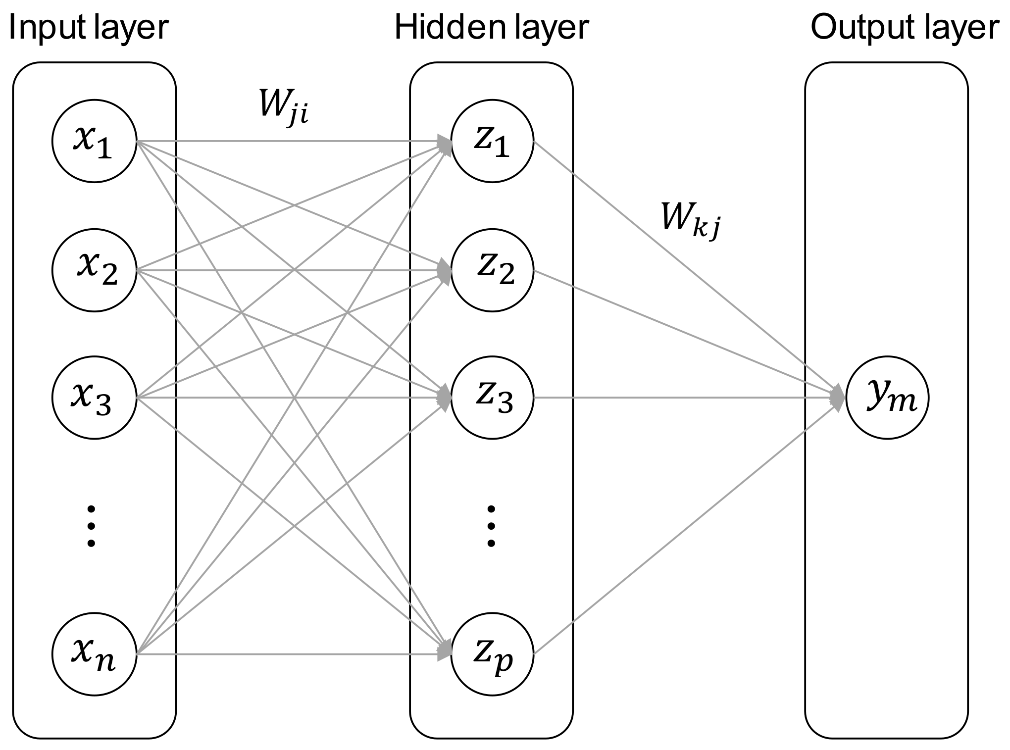
2.3. Artificial Neural Network (ANN) Model
2.4. Adaptive Neural-Based Fuzzy Inference System (ANFIS) Model
- Rule 1: if isandisthen
- Rule 2: ifisandisthen where and are the membership functions of each input and , and are the output functions and and are linear parameters. The ANFIS model consists of five layers as shown in Figure 2.
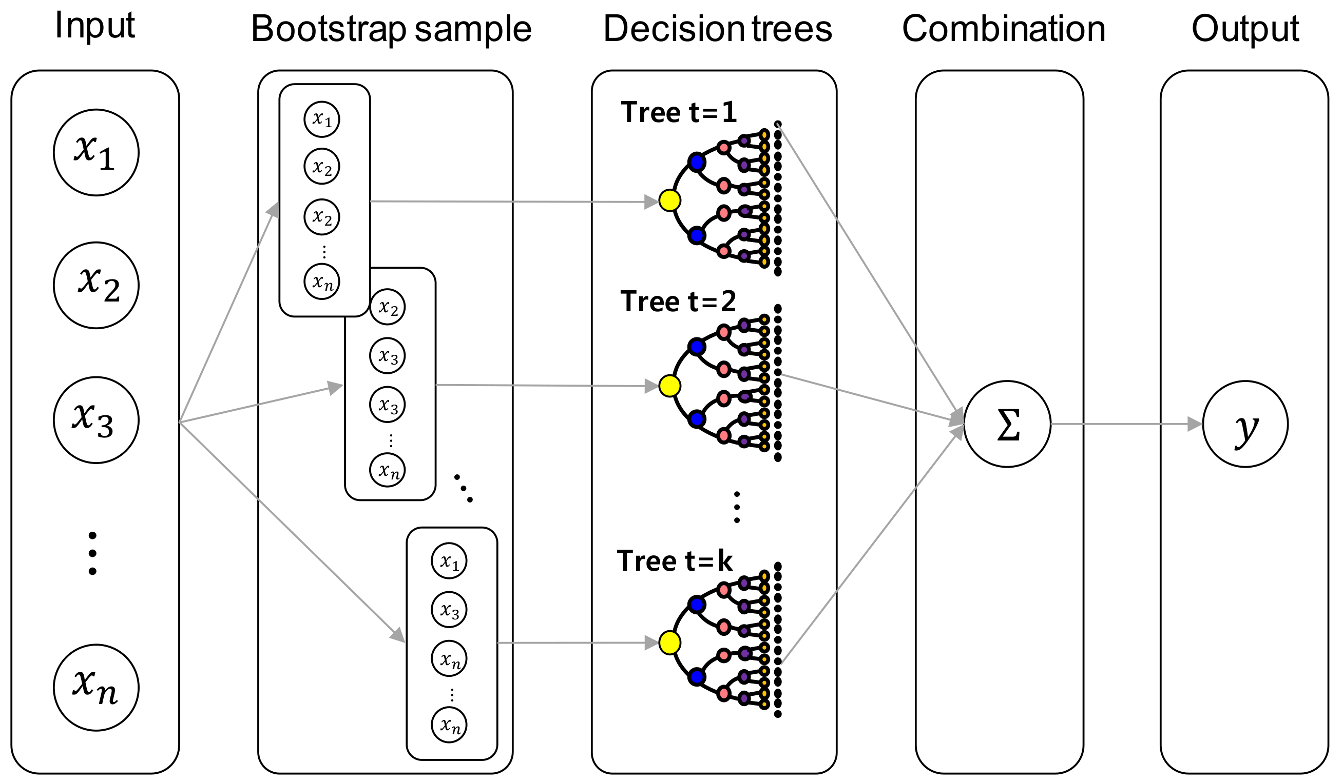
2.5. Random Forest (RF) Model
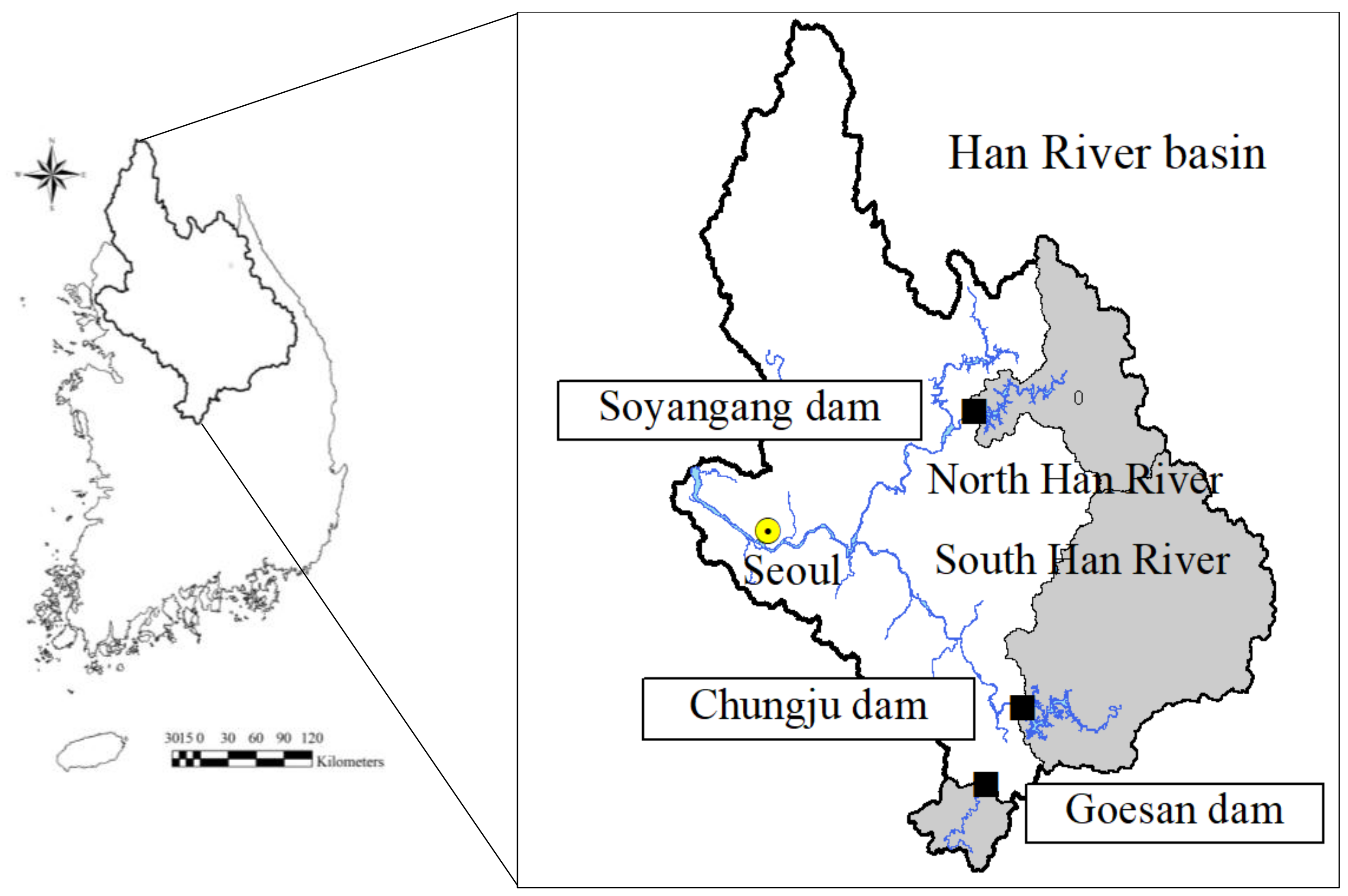
3. Data and Study Area
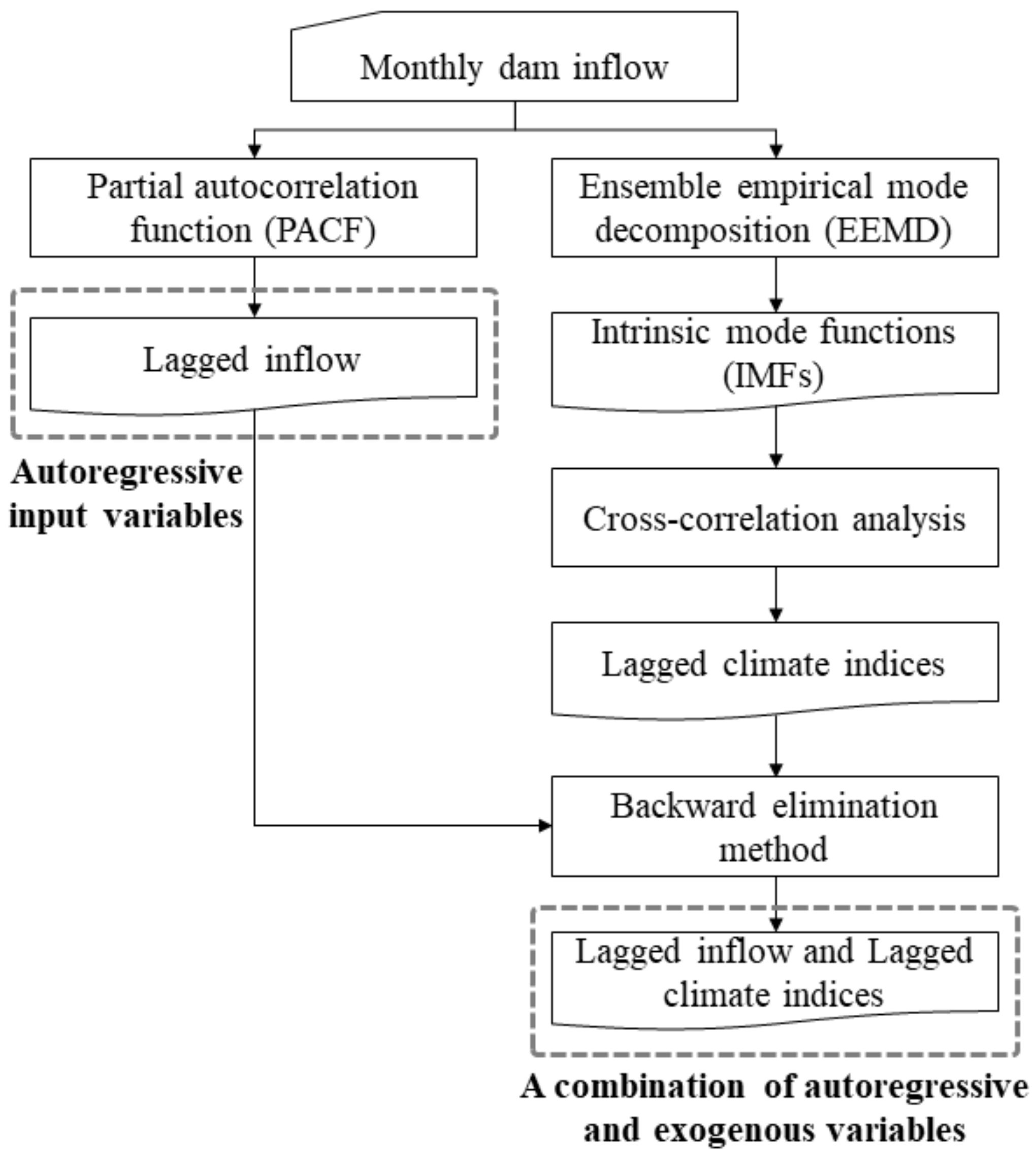
4. Input Variable Selection
4.1. Partial Autocorrelation Function (PACF)
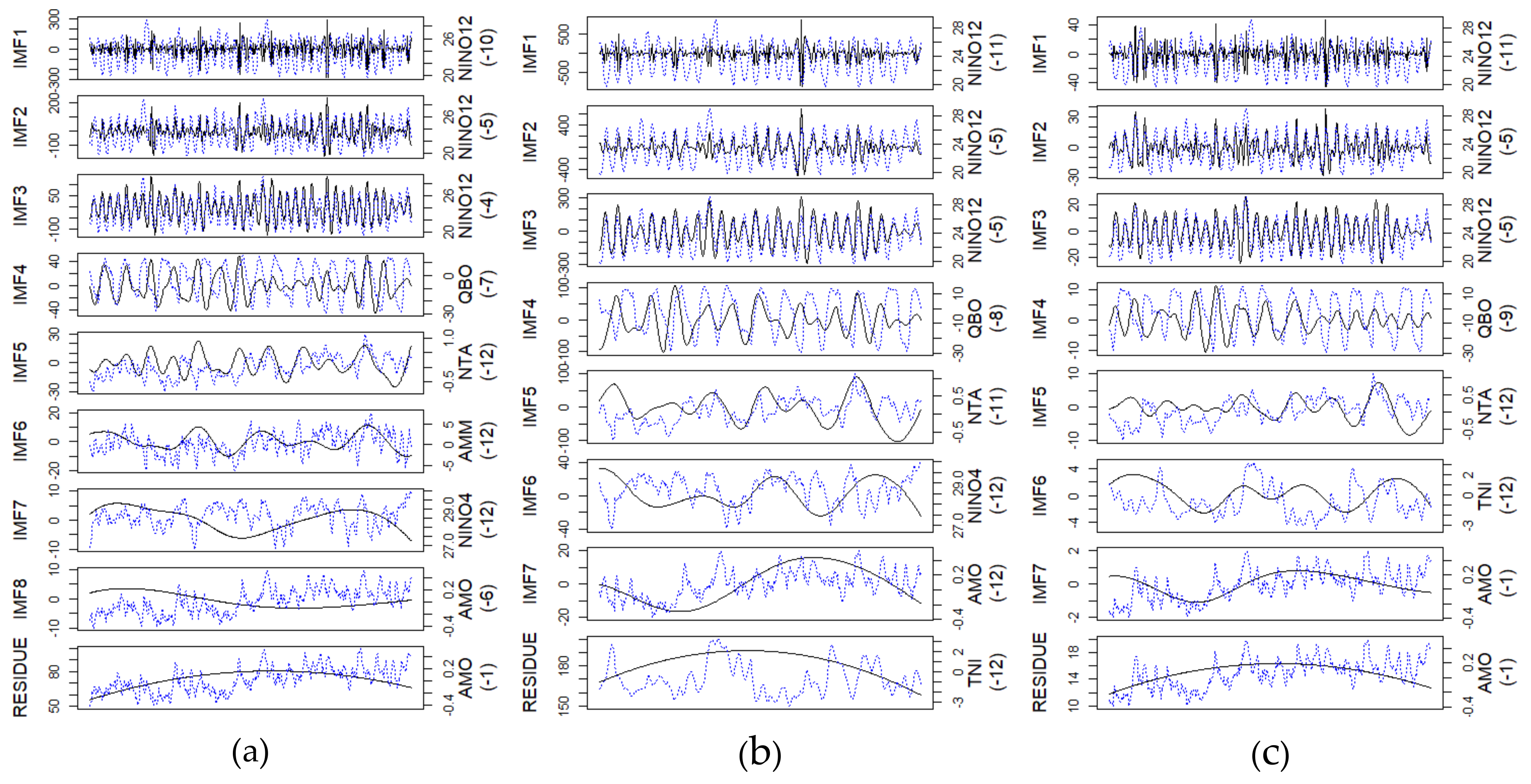
4.2. Ensemble Empirical Mode Decomposition (EEMD)
4.3. Cross-Correlation Analysis
4.4. Backward Elimination Method
5. Application and Results
5.1. Model Input Variables
5.2. Model Parameters and Setting
5.2.1. SARIMA and SARIMAX Models
5.2.2. ANN Models
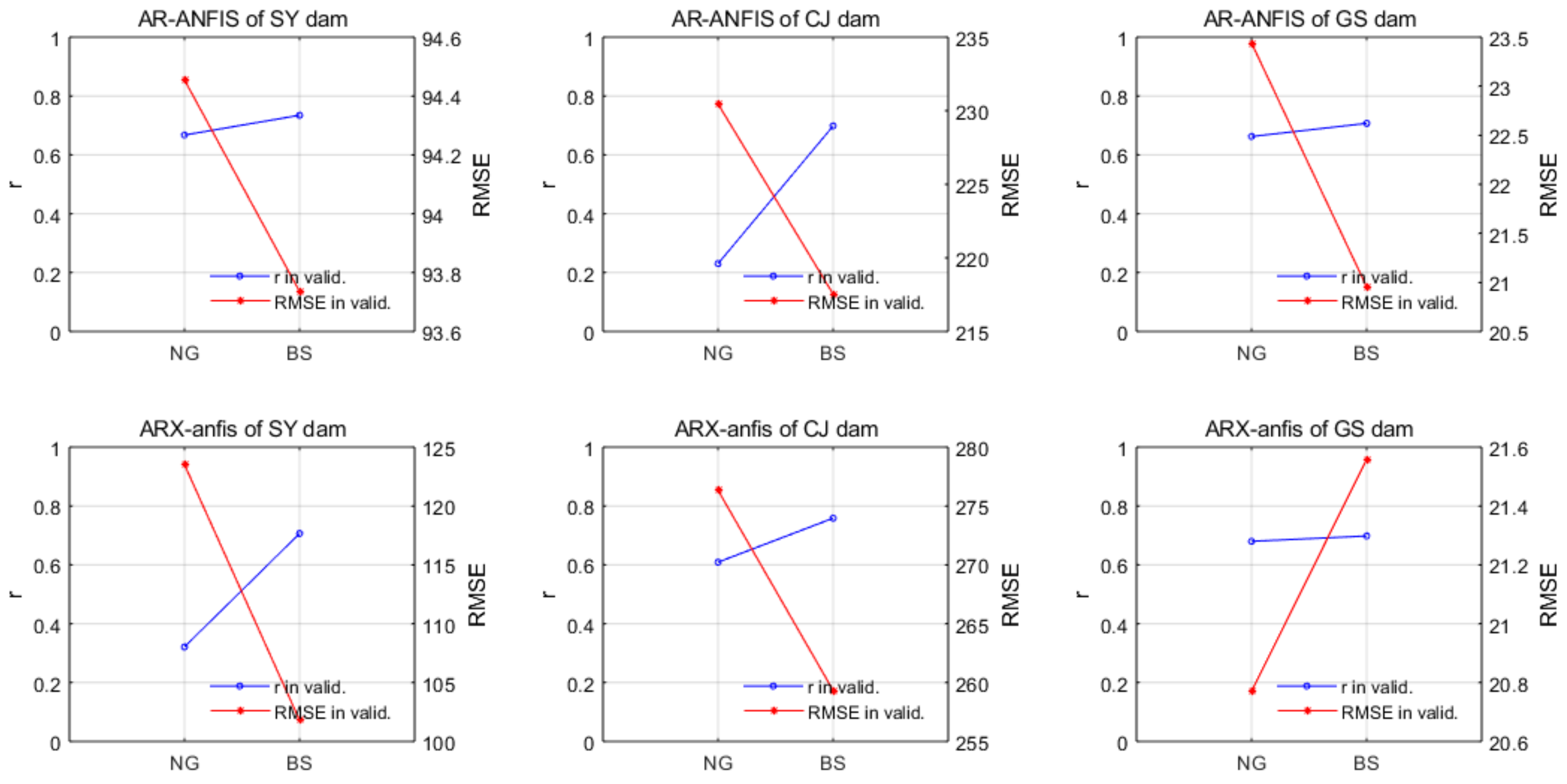
5.2.3. ANFIS Models
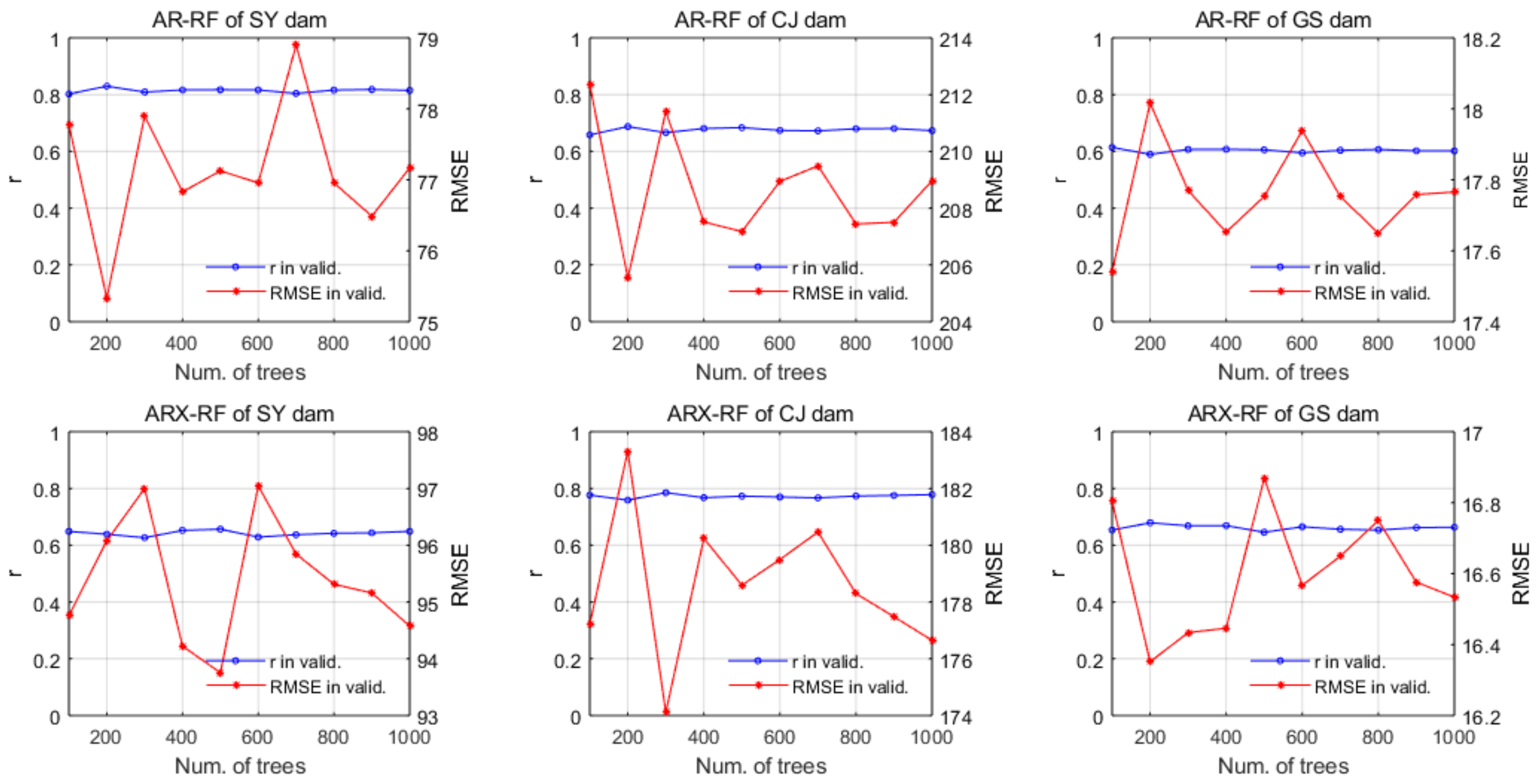
5.2.4. RF Models
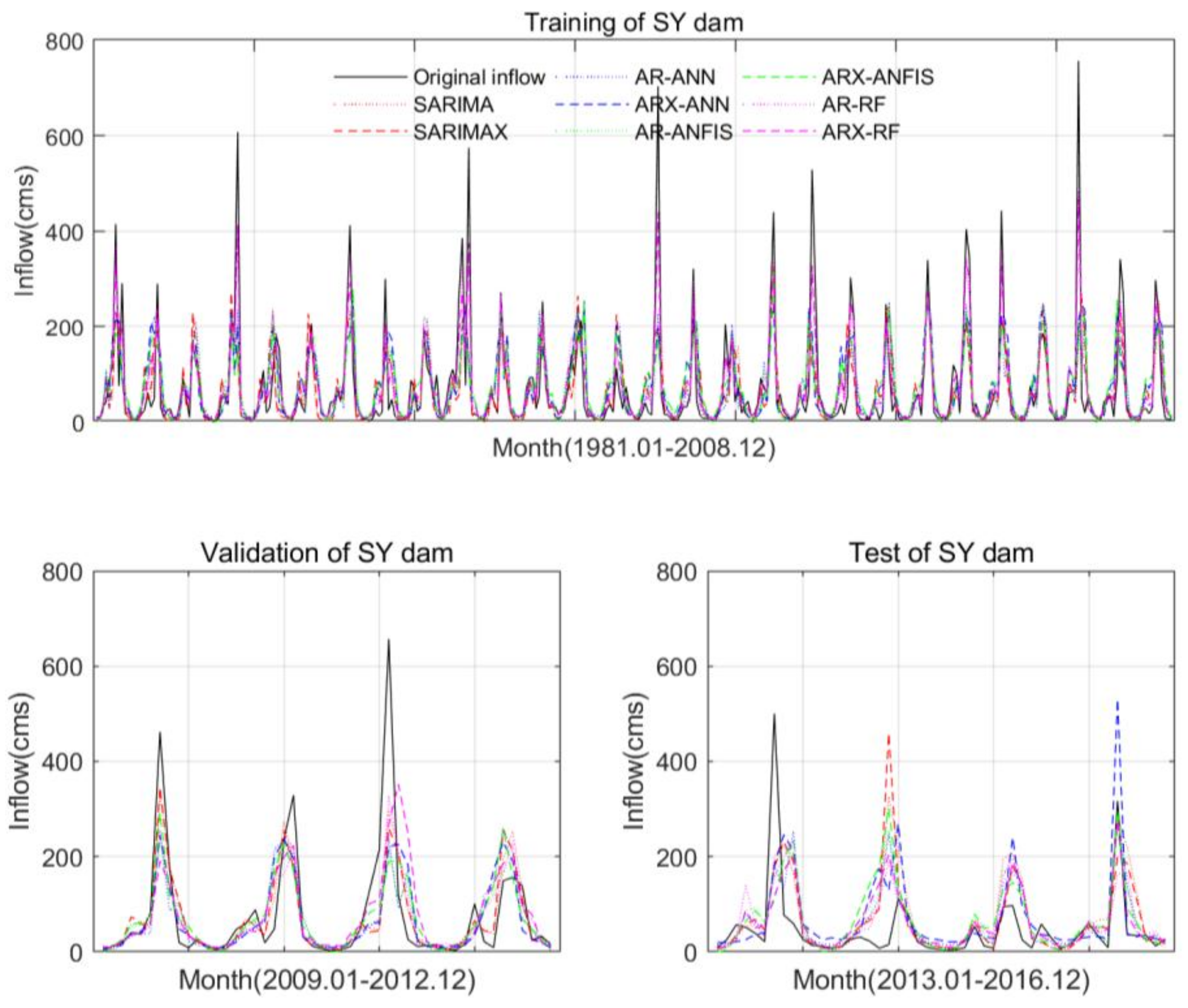
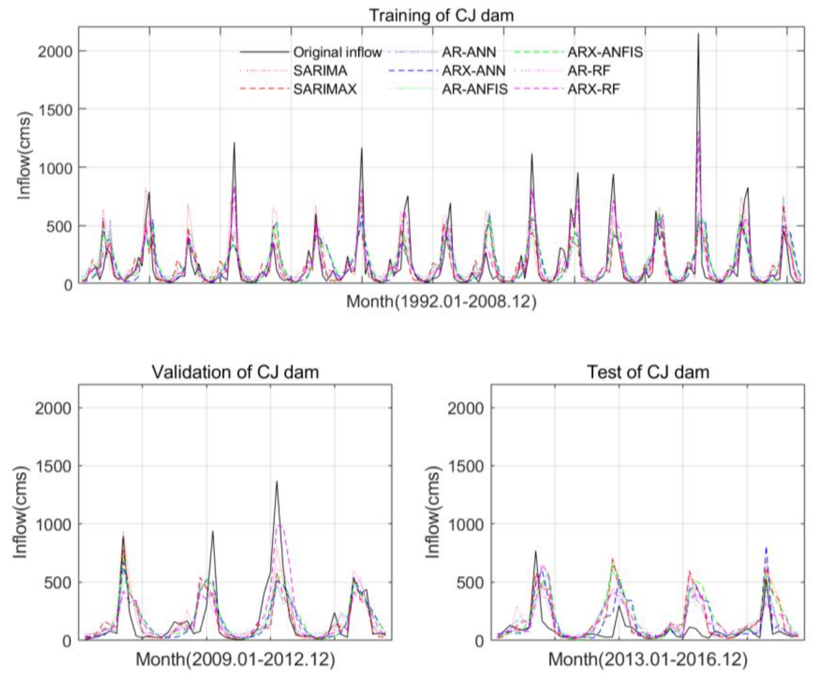
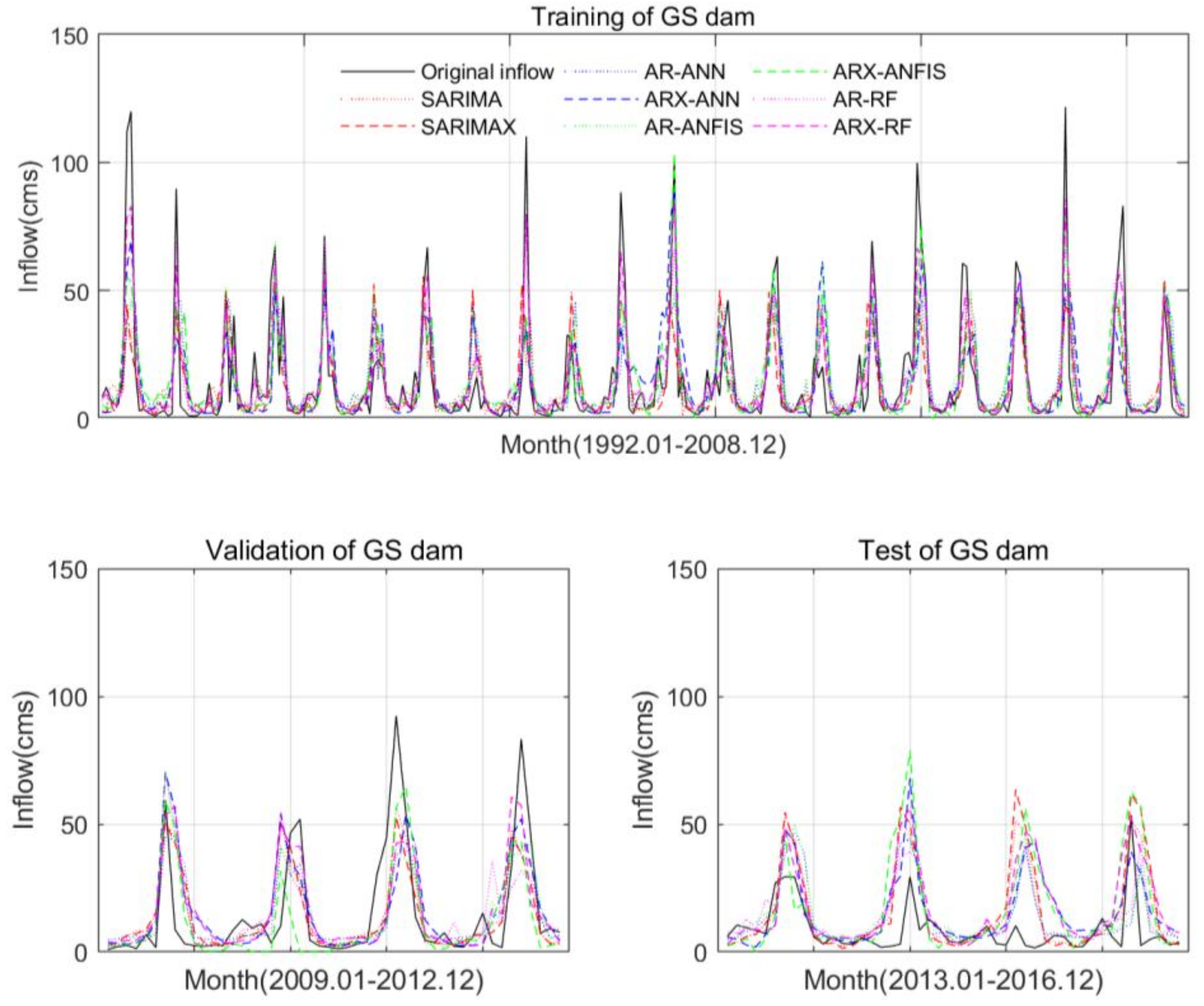
5.3. Model Performance
6. Discussion
7. Conclusions
Author Contributions
Funding
Acknowledgments
Conflicts of Interest
References
- Wang, W.-C.; Chau, K.-W.; Cheng, C.-T.; Qiu, L. A comparison of performance of several artificial intelligence methods for forecasting monthly discharge time series. J. Hydrol. 2009, 374, 294–306. [Google Scholar] [CrossRef] [Green Version]
- Wang, Y.; Guo, S.-L.; Chen, H.; Zhou, Y.-L. Comparative study of monthly inflow prediction methods for the Three Gorges Reservoir. Stoch. Environ. Res. Risk Assess. 2014, 28, 555–570. [Google Scholar] [CrossRef]
- Wang, W.C.; Chau, K.W.; Xu, D.M.; Chen, X.Y. Improving forecasting accuracy of annual runoff time series using ARIMA based on EEMD decomposition. Water Resour. Manag. 2015, 29, 2655–2675. [Google Scholar] [CrossRef]
- Valipour, M.; Banihabib, E.B.; Behbahani, S.M.R. Comparison of the ARMA, ARIMA, and the autoregressive artificial neural network models in forecasting the monthly inflow of Dez dam reservoir. J. Hydrol. 2013, 476, 433–441. [Google Scholar] [CrossRef]
- Awan, J.A.; Bae, D.-H. Improving ANFIS Based Model for Long-term Dam Inflow Prediction by Incorporating Monthly Rainfall Forecasts. Water Resour. Manag. 2014, 28, 1185–1199. [Google Scholar] [CrossRef]
- Kalteh, A.M. Wavelet Genetic Algorithm-Support Vector Regression (Wavelet GA-SVR) for Monthly Flow Forecasting. Water Resour. Manag. 2015, 29, 1283–1293. [Google Scholar] [CrossRef]
- Kisi, O. Streamflow Forecasting and Estimation Using Least Square Support Vector Regression and Adaptive Neuro-Fuzzy Embedded Fuzzy c-means Clustering. Water Resour. Manag. 2015, 29, 5109–5127. [Google Scholar] [CrossRef]
- Li, C.; Bai, Y.; Zeng, B. Deep Feature Learning Architectures for Daily Reservoir Inflow Forecasting. Water Resour. Manag. 2016, 30, 5145–5161. [Google Scholar] [CrossRef]
- Moeeni, H.; Bonakdari, H.; Ebtehai, I. Integrated SARIMA with Neuro-Fuzzy Systems and Neural Networks for Monthly Inflow Prediction. Water Resour. Manag. 2017, 31, 2141–2156. [Google Scholar] [CrossRef]
- Box, G.E.P.; Jenkins, G.M. Time Series Analysis Forecasting and Control; Holden-Day: San Francisco, CA, USA, 1970. [Google Scholar]
- Carlson, R.F.; MacCormick, A.J.A.; Watts, D.G. Application of linear random models to four annual streamflow series. Water Resour. Res. 1970, 6, 1070–1078. [Google Scholar] [CrossRef]
- Salas, J.D.; Tabios, G.Q.; Bartolini, P. Approaches to multivariate modeling of water resources time series. J. Am. Water Resour. Assoc. 1985, 21, 683–708. [Google Scholar] [CrossRef]
- Burlando, P.; Rosso, R.; Cadavid, L.G.; Salas, J.D. Forecasting of short-term rainfall using ARMA models. J. Hydrol. 1993, 144, 193–211. [Google Scholar] [CrossRef]
- Hipel, K.W.; McLeod, A.I. Time Series Modelling of Water Resources and Environmental Systems; Elsevier: Amsterdam, The Netherlands, 1994. [Google Scholar]
- Mohan, S.; Vedula, S. Multiplicative seasonal ARIMA model for longterm forecasting of inflows. Water Resour. Manag. 1995, 9, 115–126. [Google Scholar] [CrossRef]
- Papamichail, D.M.; Georgiou, P.E. Seasonal ARIMA inflow models for reservoir sizing. J. Am. Water Resour. Assoc. 2001, 37, 877–885. [Google Scholar] [CrossRef]
- Campolo, M.; Soldati, A.; Andreussi, P. Artificial neural network approach to flood forecasting in the River Arno. Hydrol. Sci. J. 2003, 48, 381–398. [Google Scholar] [CrossRef] [Green Version]
- Cheng, C.T.; Lin, J.Y.; Sun, Y.G.; Chau, K. Long-Term Prediction of Discharges in Manwan Hydropower Using Adaptive-Network-Based Fuzzy Inference Systems Models; Advances in Natural Computation; Springer: Berlin, Germany, 2005. [Google Scholar]
- Jain, A.; Kumar, A.M. Hybrid neural network models for hydrologic time series forecasting. Appl. Soft Comput. 2007, 7, 585–592. [Google Scholar] [CrossRef]
- Firat, M.; Gungör, M. Hydrological time-series modelling using an adaptive neuro-fuzzy inference system. Hydrol. Process. 2008, 22, 2122–2132. [Google Scholar] [CrossRef]
- Trichakis, I.; Nikolos, I.; Karatzas, G.P. Comparison of bootstrap confidence intervals for an ANN model of a karstic aquifer response. Hydrol. Process. 2011, 25, 2827–2836. [Google Scholar] [CrossRef]
- He, X.; Guan, H.; Zhang, X.; Simmons, C.T. A wavelet-based multiple linear regression model for forecasting monthly rainfall. Int. J. Climatol. 2014, 34, 1898–1912. [Google Scholar] [CrossRef]
- Nawaz, N.; Harun, S.; Talei, A. Application of Adaptive Network-Based Fuzzy Inference System (ANFIS) for River Stage Prediction in a Tropical Catchment. Appl. Mech. Mater. 2015, 735, 195–199. [Google Scholar] [CrossRef]
- Breiman, L. Random forest. Mach. Learn. 2001, 45, 5–32. [Google Scholar] [CrossRef]
- Yang, T.; Gao, X.; Sorooshian, S.; Li, X. Simulating California reservoir operation using the classification and regression-tree algorithm combined with a shuffled cross-validation scheme. Water Resour. Res. 2016, 52, 1626–1651. [Google Scholar] [CrossRef]
- Yang, T.; Asanjan, A.A.; Welles, E.; Gao, X.; Sorooshian, S.; Liu, X. Developing reservoir monthly inflow forecasts using artificial intelligence and climate phenomenon information. Water Rosour. Res. 2017, 53, 2786–2812. [Google Scholar] [CrossRef]
- Ahmed, J.A.; Sarma, A.K. Artificial neural network model for synthetic streamflow generation. Water Resour. Manag. 2007, 21, 1015–1029. [Google Scholar] [CrossRef]
- Noori, R.; Hoshyaripour, G.; Ashrafi, K.; Araabi, B.N. Uncertainty analysis of developed ANN and ANFIS models in prediction of carbon monoxide daily concentration. Atmos. Environ. 2010, 44, 476–482. [Google Scholar] [CrossRef]
- Valipour, M. Long-term runoff study using SARIMA and ARIMA models in the United States. Meteorol. Appl. 2015, 22, 592–598. [Google Scholar] [CrossRef] [Green Version]
- Emamgholizadeh, S.; Moslemi, K.; Karami, G. Prediction the groundwater level of Bastam Plain (Iran) by artificial neural network (ANN) and adaptive neuro fuzzy inference system (ANFIS). Water Resour. Manag. 2014, 28, 5433–5446. [Google Scholar] [CrossRef]
- Kashid, S.S.; Ghosh, S.; Maity, R. Streamflow prediction using multi-site rainfall obtained from hydroclimatic teleconnection. J. Hydrol. 2010, 395, 23–38. [Google Scholar] [CrossRef]
- Schepen, A.; Wang, Q.J.; Robertson, D. Evidence for using lagged climate indices to forecast Australian seasonal rainfall. J. Clim. 2012, 25, 1230–1246. [Google Scholar] [CrossRef]
- Mekanik, F.; Imteaz, M.A.; Gato-Trinidad, S.; Elmahdi, A. Multiple regression and artificial neural network for long-term rainfall forecasting using large scale climate modes. J. Hydrol. 2013, 503, 11–21. [Google Scholar] [CrossRef]
- Abbot, J.; Marohasy, J. Input selection and optimisation for monthly rainfall forecasting in Queensland, Australia, using artificial neural networks. Atmos. Res. 2014, 138, 166–178. [Google Scholar] [CrossRef]
- Li, J.; Liu, X.; Chen, F. Evaluation of nonstationarity in annual maximum flood series and the associations with large-scale climate patterns and human activities. Water Resour. Manag. 2015, 29, 1653–1668. [Google Scholar] [CrossRef]
- Wu, Z.; Huang, N.E.; Long, S.R.; Peng, C.K. On the trend, detrending, and variability of nonlinear and nonstationary time series. Proc. Natl. Acad. Sci. USA 2007, 104, 14889–14894. [Google Scholar] [CrossRef] [Green Version]
- Lee, T.; Ouarda, T.B.M.J. Long-term prediction of precipitation and hydrologic extremes with nonstationary oscillation processes. J. Geophys. Res. Atmos. 2010, 115, D13107. [Google Scholar] [CrossRef]
- Breaker, L.C.; Ruzmaikin, A. The 154-year record of sea level at San Francisco: Extracting the long-term trend, recent changes, and other tidbits. Clim. Dyn. 2011, 36, 545–559. [Google Scholar] [CrossRef]
- Shi, F.; Yang, B.; Gunten, L.; Qin, C.; Wang, Z. Ensemble empirical mode decomposition for tree-ring climate reconstructions. Theor. Appl. Climatol. 2012, 109, 233–243. [Google Scholar] [CrossRef]
- Castino, F.; Bookhagen, B.; Strecker, M.R. Oscillations and trends of river discharge in the southern Central Andes and linkages with climate variability. J. Hydrol. 2017, 555, 108–124. [Google Scholar] [CrossRef]
- Kim, T.; Shin, J.-Y.; Kim, S.; Heo, J.-H. Identification of relationships between climate indices and long-term precipitation in South Korea using ensemble empirical mode decomposition. J. Hydrol. 2018, 557, 726–739. [Google Scholar] [CrossRef]
- Yu, X.; Zhang, X.; Qin, H. A Data-driven Model Based on Fourier Transform and Support Vector Regression for Monthly Reservoir Inflow Forecasting. J. Hydro-Environ. Res. 2018, 18, 12–24. [Google Scholar] [CrossRef]
- Jalalkamali, A.; Moradi, M.; Moradi, N. Application of several artificial intelligence models and ARIMAX model for forecasting drought using the Standardized Precipitation Index. Int. J. Environ. Sci. Technol. 2015, 12, 1201–1210. [Google Scholar] [CrossRef]
- Yang, T.; Asanjan, A.A.; Faridzad, M.; Hayatbini, N.; Gao, X.; Sorooshian, S. An enhanced artificial neural network with a shuffled complex evolutionary global optimization with principal component analysis. Inform. Sci. 2017, 418–419, 302–316. [Google Scholar] [CrossRef]
- Avarideh, F. Application of Hydro-Informatics in Sediment Transport. Ph.D. Thesis, Amirkabir University of Technology, Tehran, Iran, 2012. [Google Scholar]
- Jang, J.S.R. ANFIS: Adaptive-Network-Based Fuzzy Inference System. IEEE Trans. Syst. Man. Cybern. 1993, 23, 665–685. [Google Scholar] [CrossRef]
- Wang, L.; Zhou, X.; Zhu, X.; Dong, Z.; Guo, W. Estimation of biomass in wheat using random forest regression algorithm and remote sensing data. Crop J. 2016, 4, 212–219. [Google Scholar] [CrossRef] [Green Version]
- Huang, N.E.; Shen, Z.; Long, S.R.; Wu, M.C.; Shih, H.H.; Zheng, Q.; Yen, N.C.; Tung, C.C.; Liu, H.H. The empirical mode decomposition method and the Hilbert spectrum for non-stationary time series analysis. Proc. Math. Phys. Eng. Sci. 1998, 354, 903–995. [Google Scholar] [CrossRef]
- Wu, Z.; Huang, N.E. Ensemble empirical mode decomposition: A noise-assisted data analysis method. Adv. Adapt. Data Anal. 2009, 1, 1–41. [Google Scholar] [CrossRef]
- May, R.; Dandy, G.; Maier, H. Review of Input Variable Selection Methods for Artificial Neural Networks. In Artificial Neural Networks-Methodological Advances and Biomedical Applications; Kenji, S., Ed.; InTechOpen: London, UK, 2011; ISBN 978-953-307-243-2. [Google Scholar] [Green Version]
- Cryer, J.D.; Chan, K.S. Time Series Analysis with Applications in R, 2nd ed.; Springer: New York, NY, USA, 2008; ISBN 978-0-387-75959-3. [Google Scholar]
- Sgurev, V.; Yager, R.R.; Kacprzyk, J.; Jotsov, V. Innovative Issues in Intelligent Systems; Springer: Cham, Switzerland, 2016; ISBN 978-3-319-27267-2. [Google Scholar]
- Lee, T.; Ouarda, T.B.M.J. Stochastic simulation of nonstationary oscillation hydro-climatic processes using empirical mode decomposition. Water Resour. Res. 2012, 48, W02514. [Google Scholar] [CrossRef]
- Kim, Y.; Cho, K. Sea level rise around Korea: Analysis of tide gauge station data with the ensemble empirical mode decomposition method. J. Hydro-Environ. Res. 2016, 11, 138–145. [Google Scholar] [CrossRef]
- Zhang, D.; Lin, J.; Peng, Q.; Wang, D.; Yang, T.; Sorooshian, S.; Liu, X.; Zhuang, J. Modeling and simulating of reservoir operation using the artificial neural network, support vector regression, deep learning algorithm. J. Hydrol. 2018, 565, 720–736. [Google Scholar] [CrossRef]


| Station | Type | Data Period | Basin Area (km2) | Volume (×103 m3) | Water Supply Capacity (×103 m3) | Mean Inflow (m3/s) | |
|---|---|---|---|---|---|---|---|
| Annual | Seasonal (JJAS) | ||||||
| Soyangang dam | Multi-purpose (E.C.R.Da) | January 1974–December 2016 | 2703 | 9600 | 1,900,000 | 68.28 | 221.99 |
| Chungju dam | Multi-purpose (C.G.Db) | January 1986–December 2016 | 6705 | 902 | 1,789,000 | 162.39 | 359.22 |
| Goesan dam | Hydro-power (C.G.Db) | January 1982–December 2016 | 671 | 19.6 | 5700 | 13.72 | 30.18 |
| Climate Index | Classification | Climate Index | Classification |
|---|---|---|---|
| NINO 1+2 (NINO12) | ENSO/SST:Pacific | Tropical Northern Atlantic Index (TNA) | SST:Atlantic |
| NINO 3 (NINO3) | ENSO/SST:Pacific | Tropical Southern Atlantic Index (TSA) | SST:Atlantic |
| NINO 4 (NINO4) | ENSO/SST:Pacific | Carribbean SST Index (CAR) | SST:Atlantic |
| NINO 3.4 (NINO34) | ENSO/SST:Pacific | Pacific Decadal Oscillation (PDO) | Teleconnections |
| Bivariate ENSO Timeseries (BEST) | ENSO | Northern Oscillation Index (NOI) | Teleconnections |
| Multivariate ENSO Index (MEI) | ENSO | Pacific North American Index (PNA) | Teleconnections |
| Trans-Nino Index (TNI) | SST:Pacific | Western Pacific Index (WP) | Teleconnections |
| Western Hemisphere Warm Pool (WHWP) | SST:Pacific/SST:Atlantic | Eastern Atlantic/Western Russia (EAWR) | Teleconnections |
| Oceanic Nino Index (ONI) | SST:Pacific | North Atlantic Oscillation (NAO) | Teleconnections |
| Atlantic Multidecadal Oscillation (AMO) | SST:Atlantic | Southern Oscillation Index (SOI) | Atmosphere |
| Atlantic Meridional Mode (AMM) | SST:Atlantic | Quasi-Biennial Oscillation (QBO) | Atmosphere |
| North Tropical Atlantic SST Index (NTA) | SST:Atlantic | Artic Oscillation (AO) | Atmosphere |
| Station | Autoregressive Variables (AR-) | A Combination of Autoregressive and Exogenous Variables (ARX-) |
|---|---|---|
| SY dam | Lag1, Lag12, Lag24, Lag36 | Lag12, Lag36, NTA(12), AMO(6), NINO4(12), NINO12(10), AMM(12) |
| CJ dam | Lag36, TNI(12), AMO(12), NINO12(11), NTA(11), NINO12(5) | |
| GS dam | Lag12, Lag36, NINO12(5), QBO(9), AMO(1) |
| SY Dam | CJ Dam | GS Dam | |||||||||
|---|---|---|---|---|---|---|---|---|---|---|---|
| IMFs | CI | Lag | r | IMFs | CI | Lag | r | IMFs | CI | Lag | r |
| IMF1 | NINO12 | 10 | 0.21 | IMF1 | NINO12 | 11 | 0.22 | IMF1 | NINO12 | 11 | 0.19 |
| IMF2 | NINO12 | 5 | 0.42 | IMF2 | NINO12 | 5 | 0.48 | IMF2 | NINO12 | 5 | 0.45 |
| IMF3 | NINO12 | 4 | 0.76 | IMF3 | NINO12 | 5 | 0.75 | IMF3 | NINO12 | 5 | 0.75 |
| IMF4 | QBO | 7 | −0.32 | IMF4 | QBO | 8 | −0.33 | IMF4 | QBO | 9 | −0.29 |
| IMF5 | NTA | 12 | −0.21 | IMF5 | NTA | 11 | −0.42 | IMF5 | NTA | 12 | −0.40 |
| IMF6 | AMM | 12 | −0.29 | IMF6 | NINO4 | 12 | −0.38 | IMF6 | TNI | 12 | 0.32 |
| IMF7 | NINO4 | 12 | −0.15 | IMF7 | AMO | 12 | 0.49 | IMF7 | AMO | 1 | 0.30 |
| IMF8 | AMO | 6 | −0.57 | RES | TNI | 12 | −0.21 | RES | AMO | 1 | 0.25 |
| RES | AMO | 1 | 0.47 | ||||||||
| Station | SARIMA (p, d, q)(P, D, Q)[s] | SARIMAX (p, d, q)(P, D, Q)[s] |
|---|---|---|
| SY dam | SARIMA(0,0,0)(2,1,2)[12] | SARIMAX(0,0,0)(3,1,1)[12]. Lag12 |
| −0.926, −0.271, −0.155, −0.732 | −0.117, −0.202, 0.148, −0.954, 0.326 | |
| CJ dam | SARIMA(0,0,0)(1,1,3)[12] | SARIMAX(0,0,0)(2,1,1)[12] Lag36 |
| −0.758, −0.147, −0.887, 0.148 | −0.071, 0.052, −0.949, 0.133 | |
| GS dam | SARIMA(0,0,1)(1,1,1)[12] | SARIMAX(0,0,0)(1,1,1)[12] Lag12 |
| 0.171, −0.066, −0.888 | 0.152, −0.937, −0.254 |
| Station | AR-ANN | ARX-ANN |
|---|---|---|
| SY dam | 3 | 5 |
| CJ dam | 4 | 4 |
| GS dam | 2 | 2 |
| Station | AR-ANFIS | ARX-ANFIS | ||||
|---|---|---|---|---|---|---|
| Optimal MF | Number of Input MF (Layer2) | Number of Rules (Layer3) | Optimal MF | Number of Input MF (Layer2) | Number of Rules (Layer3) | |
| SY dam | BS | 8 | 16 | BS | 14 | 128 |
| CJ dam | BS | 8 | 16 | BS | 12 | 64 |
| GS dam | BS | 8 | 16 | NG | 10 | 32 |
| Station | AR-RF | ARX-RF |
|---|---|---|
| SY dam | 200 | 500 |
| CJ dam | 200 | 300 |
| GS dam | 100 | 200 |
| Station | Model | r | RMSE | NSE | ||||||
|---|---|---|---|---|---|---|---|---|---|---|
| Train. | Vali. | Test | Train. | Vali. | Test | Train. | Vali. | Test | ||
| SY dam | SARIMA | 0.65 | 0.53 | 84.17 | 83.69 | 0.42 | −0.04 | |||
| SARIMAX | 0.65 | 0.38 | 84.52 | 93.82 | 0.42 | −0.31 | ||||
| AR-ANN | 0.66 | 0.70 | 0.58 | 82.89 | 89.18 | 72.28 | 0.44 | 0.49 | 0.22 | |
| ARX-ANN | 0.64 | 0.68 | 0.63 | 85.56 | 91.63 | 80.64 | 0.40 | 0.46 | 0.03 | |
| AR-ANFIS | 0.65 | 0.73 | 0.53 | 84.54 | 88.49 | 74.97 | 0.42 | 0.49 | 0.16 | |
| ARX-ANFIS | 0.61 | 0.71 | 0.41 | 87.93 | 89.53 | 86.96 | 0.37 | 0.48 | −0.13 | |
| AR-RF | 0.94 | 0.83 | 0.47 | 42.61 | 75.33 | 77.78 | 0.85 | 0.63 | 0.10 | |
| ARX-RF | 0.95 | 0.66 | 0.50 | 42.45 | 93.76 | 75.71 | 0.85 | 0.43 | 0.15 | |
| CJ dam | SARIMA | 0.65 | 0.57 | 203.35 | 179.26 | 0.41 | −0.93 | |||
| SARIMAX | 0.63 | 0.57 | 205.62 | 180.51 | 0.40 | −0.96 | ||||
| AR-ANN | 0.64 | 0.71 | 0.52 | 204.71 | 202.42 | 162.32 | 0.40 | 0.48 | −0.58 | |
| ARX-ANN | 0.61 | 0.74 | 0.67 | 209.49 | 191.73 | 151.26 | 0.37 | 0.53 | −0.37 | |
| AR-ANFIS | 0.63 | 0.70 | 0.46 | 205.29 | 208.25 | 162.20 | 0.40 | 0.45 | −0.58 | |
| ARX-ANFIS | 0.64 | 0.76 | 0.41 | 203.89 | 186.34 | 203.91 | 0.41 | 0.56 | −1.50 | |
| AR-RF | 0.93 | 0.68 | 0.42 | 110.41 | 207.17 | 157.52 | 0.83 | 0.46 | −0.49 | |
| ARX-RF | 0.93 | 0.79 | 0.40 | 108.83 | 174.11 | 169.53 | 0.83 | 0.62 | −0.73 | |
| GS dam | SARIMA | 0.65 | 0.52 | 17.44 | 15.55 | 0.42 | −1.56 | |||
| SARIMAX | 0.67 | 0.51 | 17.14 | 17.86 | 0.44 | −2.38 | ||||
| AR-ANN | 0.62 | 0.72 | 0.37 | 17.88 | 15.37 | 13.67 | 0.39 | 0.51 | −0.98 | |
| ARX-ANN | 0.69 | 0.63 | 0.51 | 16.48 | 17.41 | 14.21 | 0.48 | 0.37 | −1.14 | |
| AR-ANFIS | 0.65 | 0.71 | 0.35 | 17.31 | 15.58 | 14.37 | 0.43 | 0.50 | −1.19 | |
| ARX-ANFIS | 0.77 | 0.68 | 0.42 | 14.77 | 16.69 | 19.40 | 0.58 | 0.42 | −2.99 | |
| AR-RF | 0.93 | 0.59 | 0.38 | 9.13 | 18.02 | 13.45 | 0.84 | 0.33 | −0.92 | |
| ARX-RF | 0.94 | 0.68 | 0.46 | 8.69 | 16.35 | 16.76 | 0.86 | 0.45 | −1.98 | |
| Station | Model | r | RMSE | NSE | |||||||||
|---|---|---|---|---|---|---|---|---|---|---|---|---|---|
| 2013 | 2014 | 2015 | 2016 | 2013 | 2014 | 2015 | 2016 | 2013 | 2014 | 2015 | 2016 | ||
| SY dam | SARIMA | 0.62 | 0.43 | 0.78 | 0.75 | 102.18 | 99.57 | 59.86 | 63.84 | 0.38 | −9.02 | −2.31 | 0.38 |
| SARIMAX | 0.53 | 0.10 | 0.67 | 0.69 | 110.61 | 131.76 | 43.73 | 60.81 | 0.28 | −16.54 | −0.77 | 0.44 | |
| AR-ANN | 0.53 | 0.18 | 0.75 | 0.93 | 110.56 | 75.68 | 43.94 | 31.80 | 0.28 | −4.79 | −0.79 | 0.85 | |
| ARX-ANN | 0.50 | 0.58 | 0.71 | 0.99 | 114.18 | 80.57 | 49.75 | 63.31 | 0.23 | −5.56 | −1.29 | 0.39 | |
| AR-ANFIS | 0.50 | 0.23 | 0.80 | 0.90 | 112.66 | 80.56 | 44.31 | 36.59 | 0.25 | −5.56 | −0.82 | 0.80 | |
| ARX-ANFIS | 0.27 | 0.14 | 0.75 | 0.96 | 130.77 | 104.71 | 39.43 | 25.02 | −0.01 | −10.08 | −0.44 | 0.91 | |
| AR-RF | 0.41 | 0.29 | 0.82 | 0.68 | 121.48 | 58.62 | 49.12 | 59.95 | 0.13 | −2.47 | −1.23 | 0.45 | |
| ARX-RF | 0.36 | 0.21 | 0.69 | 0.97 | 122.78 | 72.36 | 45.84 | 22.66 | 0.11 | −4.29 | −0.94 | 0.92 | |
| CJ dam | SARIMA | 0.81 | 0.45 | 0.58 | 0.76 | 115.63 | 227.95 | 189.39 | 165.34 | 0.64 | −7.96 | −28.82 | −0.52 |
| SARIMAX | 0.75 | 0.40 | 0.59 | 0.78 | 140.97 | 221.25 | 204.75 | 139.94 | 0.47 | −7.45 | −33.85 | −0.09 | |
| AR-ANN | 0.58 | 0.38 | 0.64 | 0.83 | 181.56 | 210.36 | 147.21 | 80.67 | 0.12 | −6.63 | −17.02 | 0.64 | |
| ARX-ANN | 0.62 | 0.83 | 0.42 | 0.99 | 169.29 | 137.67 | 190.67 | 86.89 | 0.23 | −2.27 | −29.22 | 0.58 | |
| AR-ANFIS | 0.54 | 0.30 | 0.68 | 0.76 | 182.45 | 214.87 | 131.65 | 91.90 | 0.11 | −6.96 | −13.41 | 0.53 | |
| ARX-ANFIS | 0.39 | 0.50 | 0.45 | 0.74 | 212.50 | 237.39 | 211.93 | 141.02 | −0.21 | −8.72 | −36.34 | −0.10 | |
| AR-RF | 0.43 | 0.36 | 0.66 | 0.78 | 182.52 | 167.42 | 172.71 | 89.85 | 0.11 | −3.84 | −23.80 | 0.55 | |
| ARX-RF | 0.35 | 0.47 | 0.61 | 0.69 | 230.87 | 162.34 | 153.13 | 108.92 | −0.43 | −3.55 | −18.49 | 0.34 | |
| GS dam | SARIMA | 0.87 | 0.47 | 0.05 | 0.62 | 9.52 | 16.66 | 19.43 | 14.87 | −0.02 | −4.11 | −49.30 | −0.16 |
| SARIMAX | 0.88 | 0.48 | 0.10 | 0.62 | 9.32 | 18.26 | 22.81 | 18.30 | 0.02 | −5.14 | −68.31 | −0.75 | |
| AR-ANN | 0.82 | 0.50 | −0.21 | 0.01 | 10.10 | 15.14 | 13.00 | 15.70 | −0.15 | −3.22 | −21.52 | −0.29 | |
| ARX-ANN | 0.82 | 0.79 | −0.39 | 0.71 | 8.89 | 15.67 | 18.74 | 11.49 | 0.11 | −3.52 | −45.80 | 0.31 | |
| AR-ANFIS | 0.79 | 0.44 | −0.20 | 0.10 | 10.11 | 17.06 | 14.50 | 14.90 | −0.15 | −4.36 | −27.00 | −0.16 | |
| ARX-ANFIS | 0.77 | 0.58 | −0.33 | 0.57 | 8.11 | 24.36 | 21.03 | 20.11 | 0.26 | −9.93 | −57.96 | −1.12 | |
| AR-RF | 0.85 | 0.46 | 0.02 | 0.11 | 7.63 | 14.51 | 13.74 | 16.29 | 0.34 | −2.88 | −24.17 | −0.39 | |
| ARX-RF | 0.80 | 0.61 | -0.16 | 0.59 | 7.98 | 18.23 | 20.88 | 17.07 | 0.28 | −5.12 | −57.10 | −0.52 | |
© 2019 by the authors. Licensee MDPI, Basel, Switzerland. This article is an open access article distributed under the terms and conditions of the Creative Commons Attribution (CC BY) license (http://creativecommons.org/licenses/by/4.0/).
Share and Cite
Kim, T.; Shin, J.-Y.; Kim, H.; Kim, S.; Heo, J.-H. The Use of Large-Scale Climate Indices in Monthly Reservoir Inflow Forecasting and Its Application on Time Series and Artificial Intelligence Models. Water 2019, 11, 374. https://doi.org/10.3390/w11020374
Kim T, Shin J-Y, Kim H, Kim S, Heo J-H. The Use of Large-Scale Climate Indices in Monthly Reservoir Inflow Forecasting and Its Application on Time Series and Artificial Intelligence Models. Water. 2019; 11(2):374. https://doi.org/10.3390/w11020374
Chicago/Turabian StyleKim, Taereem, Ju-Young Shin, Hanbeen Kim, Sunghun Kim, and Jun-Haeng Heo. 2019. "The Use of Large-Scale Climate Indices in Monthly Reservoir Inflow Forecasting and Its Application on Time Series and Artificial Intelligence Models" Water 11, no. 2: 374. https://doi.org/10.3390/w11020374