Composition and Dynamics of Phytoplankton in the Coastal Bays of Maryland, USA, Revealed by Microscopic Counts and Diagnostic Pigments Analyses

Abstract

Maryland Coastal Bays (MCBs) have undergone changes in water quality in the past two decades due to nutrient enrichment but the composition and dynamics of the phytoplankton community have not been adequately described. Microscopic counts and photosynthetic pigments of samples collected monthly in 2012 at selected sites in MCBs that differed with regard to the degree of anthropogenic impacts were examined. Sixty-three (63) phytoplankton genera were recorded, of which 40 species are being reported for the first time in the Bays. Among the dominant species were Dactyliosolen fragilissimus (Bacillariophyta), Paulinella ovalis (Cercozoa) and Cryptomonas sp. (Cryptophyta). Bloom densities of Heterocapsa rotundata (Miozoa), which previously had not been reported in the Bays, were observed bay-wide in December, particularly at the mouth of St. Martin River. Diatoms dominated (>40%) the phytoplankton community in winter and decreased in spring (<40%), while Cercozoa and microphytoflagellates (MPF) co-dominated in summer (July). From August to October, diatoms dominated with maximum contributions from an unidentified small (<10 µM) centric species and co-dominated the assemblage with cryptophytes in late fall (November). Canonical correspondence analysis indicated that diatoms were favored by high salinity and total dissolved phosphorus (TDP), cercozoans and chlorophytes by total dissolved nitrogen (TDN) and cryptophytes by dissolved organic carbon. The spatial and seasonal differences in the composition of phytoplankton species, coupled with the occurrence of potentially toxic species and bloom densities of H. rotundata suggest that important changes have occurred in the phytoplankton assemblage that likely have affected the food web of these eutrophic bays.

1. Introduction

Understanding the variation of species composition and biomass of phytoplankton gives insight into the structure and dynamics of productive aquatic ecosystems such as coastal lagoons, as these organisms regulate the structure and efficiency of food webs and are particularly vulnerable to cultural eutrophication [1,2]. Changes in temperature, salinity, amount of sunlight and the availability of specific nutrients affect phytoplankton abundance and distribution [3] as well as the occurrence and frequency of harmful algal blooms [4,5]. Microscopic techniques allow the identification and characterization of phytoplankton to the species level, although this process is strenuous and fragile species do not survive the procedural rigors [6,7], necessitating the first use of chlorophyll a as a measure of biomass [8] and more recently the use of pigment signatures from high performance liquid chromatography, HPLC [9,10,11,12,13].

The HPLC technique measures the contributions of chloro- and carotenoid biomarker pigments, which are representatives of different algal classes, to chlorophyll a [14,15,16]. While some carotenoid pigments are unambiguous (e.g., peridinin for dinoflagellates, prasinoxanthin for prasinophytes and alloxanthin for cryptophytes), some may be indicative of more than one algal class. For example, fucoxanthin is present in diatoms, chrysophytes and prymnesiophytes while 19’-Butanoyloxyfucoxanthin is representative of pelagophytes, chrysophytes and prymnesiophytes [10,15]. Combining HPLC and microscopy thus provides a robust method for monitoring phytoplankton assemblages, yielding information which can be used to understand phytoplankton dynamics in aquatic ecosystems since the sole use of photosynthetic pigments could give misleading information [17].

Information on the phytoplankton species composition in the Maryland Coastal Bays (MCBs) has been limited to reports by the Maryland Department of Natural Resources that were produced more than a decade ago [18,19] and other studies that focused mainly on the dynamics of Brown tide Aureococcus anophagefferens [4,20,21]. No previous study has used a combination of pigment analysis and microscopic cell counts to assess seasonal changes in the community composition of phytoplankton in the Maryland Coastal lagoon system that has been subjected to increased nutrient enrichment [22,23,24] for over two decades.

The objectives of this study were to: (1) use microscopic counts and pigment markers to investigate the composition and seasonal and spatial variations of phytoplankton assemblage in the MCBs based on monthly samples collected from February–December 2012 and (2) conduct multivariate analyses to explore the relationships between key environmental factors and phytoplankton community composition and dynamics.

2. Materials and Methods

2.1. Study Location and Environmental Parameters

The Maryland Coastal Bays (MCBs) are generally shallow (<2 m mean depth) aquatic systems located on the east coast of the United States. They are separated from the Atlantic Ocean by the Assateague Barrier Islands and surrounded by a 452 km² watershed where residential areas, agriculture, forests and poultry farms are located [25]. The Ocean City water inlet divides the bays into two major parts; North and South. Chincoteague Bay, which extends from the North in Maryland to the South in Virginia [26], and Newport and Sinepuxent Bays make up the Southern Bays. The northern bays consist of Isle of Wight Bay, St. Martin River and Assawoman Bay. The Ocean City and Chincoteague Inlets connect the bays to the Atlantic Ocean. Land use in the northern bays watershed includes 30.1% agriculture, 8.9% urban/commercial, 18.4% residential and 32.1% forest areas, compared to the southern bays where it is 26.6% agriculture, 5.7% urban/commercial, 5.9% residential and 38% forest areas. Land use activities coupled with increased human population in the MCBs watershed, especially in the northern bays near Ocean City, Maryland has led to increased nutrient inputs to the bays. The Ocean City population increased from 5146 (1990) to about 7000 (2017) year round residents, though during the summer particularly on weekends, the number increases to more than 320,000 vacationers totaling over 12 million visitors annually [27,28]. Between 1996 and 2008, the mean concentrations of ammonium increased from about 1 to 7 µM L⁻¹ and that of inorganic phosphates from about 0.2 to more than 0.5 µM L⁻¹ in some of the bay segments [23]. This has caused a reduction in water quality with consequent ecosystem impacts including harmful algal blooms of the Brown tide Aureococcus anophagefferens and reduced seagrass cover [18,20,21,23]. Due to the low flushing rate of the bays, ~7% per day [29] in some bay segments, nutrients from both natural [30] and anthropogenic sources [31] that enter the bays accumulate [23]. Groundwater and the creeks and streams that discharge in the western part of the bays are the major sources of freshwater input to the system and as such salinity varies from near zero in the headwaters of Trappe Creek to more than 30 in Chincoteague Bay [25]. Because of shallow depth, the MCBs water column is well mixed by winds and tides and therefore does not display marked vertical thermal and salinity gradients. For this study, 13 sites were selected from MCBs (Figure 1) and samples for nutrients, pigments and microscopic analyses were collected monthly. The southern bay sites are sites 1–5 in Chincoteague Bay; site 6 in Newport Bay, near Trappe Creek and sites 7 and 8 in Sinepuxent Bay. The northern bay sites are site 9 in Isle of Wight Bay, site 10 near the mouth of St. Martin River and sites 11–13 in Assawoman Bay. The sites varied in mean depth (m): 1.1–1.8 (sites 2, 5, 6, 10, 12), 2.0–2.4 (sites 1, 3, 4, 7, 8, 9, 13) and 3.1 (site 11). Physical and chemical parameters (salinity, temperature, pH) were measured at each site using a YSI 6600 multi-parameter probe (Yellow Springs, OH, USA). Diagnostic pigments (

Table 1. Phytoplankton diagnostic pigments, abbreviations and their corresponding taxonomic groups. Abbreviations (Abr.) are based on the SCOR (Scientific Council for Oceanic Research) nomenclature [32].

	Pigment	Abr.	Marker for	Size (µM)
1	Peridinin	Peri	Dinoflagellates	>20
2	Fucoxanthin	Fuco	Diatoms	>20
3	19’-Butanoyloxy-Fucoxanthin	But-fuco	Pelagophytes	2–20
4	Neoxanthin	Neo	Chlorophytes	2–20
5	Prasinoxanthin	Pras	Prasinophytes	2–20
6	Violaxanthin	Viola	Chlorophytes	2–20
7	19’-Hexanoyloxy-fucoxanthin	Hex-fuco	Prymnesiophytes	2–20
8	Alloxanthin	Allo	Cryptophytes	2–20
9	Lutein	Lut	Chlorophytes	2–20
10	Zeaxanthin	Zea	Cyanobacteria	<2
11	Chlorophyll b	Chl b	Chlorophytes	<2
12	Chlorophyll a	Chl a	NS

) were obtained from DHI (Denmark) and used in the HPLC calibration. For temporal analysis, the seasons were defined as follows; winter (December and February), spring (March–May), summer (June–August) and fall (September–November).

Sample Collection

Water samples were collected using a horizontal Van Dorn water sampler (Wildco) at a depth of 0.5 m below the surface, transferred into 2 L high density polyethylene (HDPE) bottles and stored in an ice box. 250 mL of bay water was transferred into amber bottles containing 2.5 mL Lugol’s Iodine (1% final concentration) for microscopic enumeration. On arrival in the laboratory, samples for nutrient and pigment analyses were vacuum filtered onto 47 mm GF/F filters using a vacuum pump at a pressure below 40 psi and the filters kept frozen at −80 °C before extraction.

2.2. Sample Analyses

2.2.1. Nutrient Analysis

Total dissolved phosphorus (TDP) and silica (SiO₂) were determined using a HACH DR/4000 spectrophotometer. A Shimadzu Total Organic Carbon Analyzer (DOC-V CPH/CPN) coupled to a Total Nitrogen Analyzer module (TNM-1) was used to measure the dissolved organic carbon (DOC) and total dissolved nitrogen (TDN). TDN was calibrated using potassium nitrate (KNO₃) and measured by the high temperature combustion method. The detection limit for DOC was 4 µM and 1 µM for TDN. Previous studies [23,25,33] reported low (<1 µM) contribution of nitrate to the total nitrogen pool, hence, total dissolved nitrogen (TDN) was used to represent the nitrogen nutrient content.

2.2.2. HPLC Pigment Analysis

Photosynthetic pigments were extracted with 5 mL of acetone, sonicated for 30 s and allowed to sit in the dark overnight at 4 °C. Centrifugation was done using an Eppendorf Centrifuge 5415 R at 2500 rpm for 5 min. Extracts were then filtered and dried under gentle pressure using a Nitrogen evaporator. The residue was re-dissolved in 200 µL of cold methanol before injection in the HPLC. The separation of pigments was conducted on an Agilent 1100 Series HPLC following the method of Zapata et al. [34] with slight modifications. The two eluents used were: (A) methanol:acetonitrile: 0.25 M aqueous pyridine (50:25:25, v/v/v) and (B) acetonitrile: acetone 80:20 (v/v). Analytical separations were performed using a Waters Symmetry C₈ column with a solvent flow rate of 1 mL/min and an injection volume of 20 µL. Pigments were detected using a diode array detector (DAD) and a fluorescence detector (FLD) at 432 nm and 666 nm. Pigments were identified from absorbance spectra characteristics and retention times and concentrations calculated from the DAD signals and response factors generated from the calibration suite. Prior peak calibration was done using commercial standards; chlorophylls a and b from Sigma Aldrich (St. Louis, MO, USA), while the carotenoid standards were obtained from DHI (Institute for Water and Environment, Hørsholm, Denmark). The Agilent HPLC chemstation software (online) was used to control all components and record the spectral and chromatographic signals while the data were processed with the offline program of the software.

2.2.3. Phytoplankton Microscopic Identification

Depending on the sample density, subsamples of 2.8 mL to 15 mL of phytoplankton samples were allowed to settle for 3 to 24 h. Diatoms, autotrophic dinoflagellates, flagellates, nano- and picoplankton (0.2–2 µM) were identified and counted to species level (where possible) using a Zeiss IM35 inverted microscope with phase contrast and bright field illumination. Small-sized phytoplankton (picophytoplankton) with morphological features too difficult to recognize were excluded from the counts. Magnifications of 125×, 250× and 500× were used to identify and enumerate the phytoplankton community composition with a detection limit of between 30 cells L⁻¹ and 1800 cells L⁻¹.

2.2.4. Freshwater Flow

To determine the influence of freshwater discharge on water quality and phytoplankton in the MCBs, monthly discharge data for a gauged stream, the New Birch Branch near Showell, MD was downloaded from the USGS website (http://nwis.waterdata.usgs.gov/nwis/monthly/ retrieved on 11 February 2015). Stream flow rate is measured hourly as it discharges directly into Shingles Landing Prong in the St. Martin River, MD and has been used as a proxy for freshwater flow into the northern coastal bays [25].

2.2.5. Statistical Analyses

A one-way ANOVA was used to test for significant differences in the means of the nutrient and other environmental data. Tukey’s test was used for multiple mean comparisons between sites. Spearman’s rank correlation coefficient was used to examine the relationships between the phytoplankton community variation and physico-chemical variables. Principal component analysis (PCA) was used to reduce the dimensionality of the data set and the influence of several parameters on the variability of the various phytoplankton taxa was assessed using canonical correspondence analysis (CCA). The Monte Carlo permutation test (with manual forward selection procedure) was used to evaluate statistical significance of the CCA results. The dependent variables tested were the different phytoplankton species and taxonomic groups, while the physico-chemical variables were included as independent variables. The CCA test was performed using CANOCO 5 statistical software [35].

3. Results

3.1. The Physical Environment

In this study, average minimum and maximum surface temperature values (±standard error) of 5.5 ± 0.13 °C and 24.65 ± 0.30 °C were observed in March and July, respectively. From April to October, temperature was above 10 °C but dropped below that value in late fall and winter (Figure 2a). Salinity was greater than 25 from winter through summer but ranged from 20 to 27 on average during fall (Figure 2b). The decrease in salinity in fall coincided with increased freshwater input (indicative of increased precipitation) from the surrounding watersheds. Spatially, salinity was highest at Sinepuxent (sites 7,8) and Isle of Wight (site 9) Bays sites (closest to the Ocean City water Inlet) and decreased through Newport (site 6) and Assawoman (sites 11–13) Bays sites (Figure 2b). pH showed minimal variation (Figure 2c) ranging from an average of 7.8 (July) to 8.1 (December). Newport Bay (site 6) had the lowest pH (7.5), observed in September, while Assawoman Bay had the highest pH (8.3) (Figure 2c). The stream flow for Birch Branch (Figure 2d) was variable during this period, with high flows occurring in March, September, November and December and low flows from April to August.

The Chemical Environment

Table 2. Mean values of chemical variables measured; dissolved organic carbon (DOC), total dissolved nitrogen (TDN), total dissolved phosphorus (TDP) and silica. Sites 1–8 are in the southern Bays while sites 9–13 are in the northern Bays.

	DOC (µM)		TDN (µM)		TDP (µM)		Silica (µM)		TDN/TDP
Site	Mean	SE	Mean	SE	Mean	SE	Mean	SE
1	317.59	21.65	26.12	2.26	1.45	0.10	20.70	5.24	18.01
2	321.25	21.61	35.99	4.92	1.80	0.21	33.46	5.11	19.99
3	332.8	30.18	29.19	3.70	1.54	0.13	18.59	5.43	18.95
4	339.11	28.14	31.61	3.37	1.85	0.44	23.70	4.94	17.09
5	327.85	24.23	37.53	7.74	1.57	0.15	20.83	3.36	23.90
6	513.67	51.91	42.98	5.17	1.53	0.15	21.77	4.6	28.09
7	250.45	31.62	28.65	5.34	1.45	0.12	20.65	4.98	19.76
8	287.4	86.05	36.6	11.59	1.46	0.13	11.12	2.69	25.07
9	344.01	77.17	48.8	13.16	1.54	0.13	19.70	5.94	31.69
10	462.01	113.19	53.94	19.48	1.56	0.10	21.11	5.79	34.58
11	431.03	129.13	49.94	15.81	1.50	0.15	18.92	4.48	33.29
12	468.87	86.92	49.42	10.77	1.42	0.14	18.27	4.16	34.80
13	502.14	104.73	53.49	14.31	1.63	0.10	17.27	4.15	32.82

shows the concentrations of dissolved organic carbon (DOC), total dissolved nitrogen (TDN), total dissolved phosphorus (TDP) and silica. A north-south decreasing gradient was observed for DOC and TDN, while the reverse was observed for silica. TDP was slightly variable among the bays and highest concentrations were observed at the western shore sites (2 and 4) within Chincoteague Bay. The TDN/TDP ratios were higher in the northern bay than southern bay sites suggesting a higher potential of phosphorus limitation in the northern bays.

More specifically, DOC concentrations varied from about 250 µM to 514 µM. Concentrations were highest in Newport Bay (site 6) and lowest at the Sinepuxent Bay sites (7 and 8). Temporally, mean monthly concentrations of DOC increased from winter through spring, peaked in summer (July) and declined through fall (October) and early winter (December) as shown in Figure 3a. Spatially, concentrations of TDN were lowest in Chincoteague Bay (site 1, 26.12 µM) and highest in St. Martin River (site 10, 53.94 µM; Table 2). Temporally, TDN (Figure 3b) ranged from 11.39 µM to 118.36 µM, was highest in spring (April) at most sites with an average concentration of 65.5 µM and lowest in winter (December and February).

Mean values of TDP ranged from 1.42 µM (site 12) to 1.85 µM (site 4) (Table 2). Concentrations of TDP decreased from winter through spring; were highest in summer (July) and lowest in fall (October) before increasing again in early winter (Figure 3c). In July when TDP peaked, its concentrations were highest in Chincoteague Bay (sites 1–5) and decreased steadily through Sinepuxent (sites 7–8) to Assawoman Bays (sites 11–13).

Mean concentrations of silica varied between 11 µM and 33 µM (Table 2) and concentrations were generally higher (>20 µM) in the southern bays sites and lower (<20 µM) in the northern bays. Temporally, silica varied between 1.0 µM and 71.25 µM (Figure 3d). In late winter, spring and fall, dissolved silica concentrations were less than 30 µM. Peak silica concentrations were observed in July when high concentrations (>30 µM) were observed at all sites and ranged from 34.5 µM (sites 7–8) to 71.25 µM (site 9).

Based on nutrient stoichiometry, more than 90% of the 143 samples collected had a TDN:TDP (Redfield) ratio less than 45 (Figure 3e) suggesting a limitation of nitrogen as is common in most coastal marine systems. In spring (April) and fall (October), very high ratios were observed at several sites, indicating phosphorus limiting conditions. Conversely, more than 90% of the samples had a Si:TDN value that was below the threshold of 1. The highest Si:TDN ratios were observed in July (Figure 3f).

3.2. Phytoplankton Species Composition

The phytoplankton taxa identified during the study period are shown in

Table 3. Phytoplankton species composition in the Maryland Coastal Bays (2012).

Kingdom Chromista	Species	Kingdom Chromista	Species
Phylum Bacillariophyta	*Achnanthes sp. Bory	Phylum Bacillariophyta	*Hemiaulus sp. Ehrenberg
	*Actinoptychus sp. C.G. Ehrenberg		*Leptocylindrus danicus Cleve
	*Amphiprora sp. Ehrenberg		Leptocylindrus minimus Gran
	*Asterionella glacialis Castracane		*Licmophora sp. C.A. Agardh
	*Aulacoseira granulata (Ehrenberg) Simonsen		Melosira moniliformis (O.F.Müller) C. Agardh
	*Biddulphia mobiliensis (J.W.Bailey) Grunow		Melosira nummuloides C.A. Agardh
	*Cerataulina bergonii Ostenfeld		Melosira sp. C.A. Agardh
	*Chaetoceros debilis Cleve		*Minutocellus polymorphus (Hargraves & Guillard)
	Chaetoceros eibenii Grunow		*Navicula sp. J.B.M. Bory de Saint-Vincent
	Chaetoceros neogracilis S.L.VanLand.		Nitzschia pungens Grunow ex Cleve
	Chaetoceros sp. C.G. Ehrenberg		Nitzschia sp. A.H. Hassall
	Chaetoceros subtilis Cleve		*Odontella aurita (Lyngbye) C.Agardh
	*Cocconeis sp. C.G. Ehrenberg		Odontella mobilensis (Bailey) Grunow
	*Corethron criophilum Castracane		*Paralia sulcata (Ehrenberg) Cleve
	Corethron sp. Castracane		*Pleurosigma sp. W. Smith
	*Coscinodiscus sp. C.G. Ehrenberg		Pseudonitzschia sp. H. Peragallo
	Cyclotella sp. (F.T. Kützing) A. de Brébisson		*Proboscia alata (Brightwell) Sundström
	Cylindrotheca closterium (Ehrenberg) Reimann &		Rhizosolenia setigera Brightwell
	*Cymbella sp. C.A. Agardh		Rhizosolenia stolterfothii H.Peragallo
	Dactyliosolen fragilissimus (Bergon) Hasle		Rhizosolenia styliformis T.Brightwell
	Dactyliosolen sp. A.F. Castracane		Rhizosolenia hebetata F. Semipina (Hensen) Gran
	*Ditylum brightwellii (T.West) Grunow		*Schroederella delicatula (H.Peragallo) Pavillard
	*Eucampia zodiacus Ehrenberg		Skeletonema costatum (Greville) Cleve
	*Flagilaria sp. Lyngbye		*Striatella sp.
	*Guinardia flaccida (Castracane) H.Peragallo		*Tabellaria sp. Kutzing
	Guinardia delicatula (Cleve) Hasle		*Thalassionema sp.
	Gyrosigma sp. A.H. Hassall		Thalassiosira sp. Cleve
Phylum Miozoa	Alexandrium sp. Halim	Phylum Chlorophyta (Kingdom Plantae)	*Ankistrodesmus sp. Corda
	*Amphidinium crassum Lohmann		*Pediastrum duplex Meyen
	Amphidinium sphenoides Wulff		*Chlorella sp. M.Beijerinck
	*Tripos furca (Ehrenberg) F.Gómez		Pyramimonas sp. Schmarda
	Ceratium sp. Shrank		Unid. Chlorophycean sphere
	Ceratium tripos (O.F.Müller) Nitzsch		*Scenedesmus quadricauda (Turpin) Brébisson
	Dinophysis acuminata Claparède & Lachmann		Scenedesmus sp. Meyen
	Dinophysis sp. Ehrenberg	Phylum Cryptophyta (Kingdom Chromista)	Cryptomonas sp. Ehrenberg
	Diplopsalis sp. Bergh	Phylum Haptophyta (Kingdom Chromista)	Chrysochromulina sp. Lackey
	*Gonyaulax sp. Diesing	Phylum Cercozoa (Kingdom Chromista)	Paulinella ovalis (A.Wulff) P.W. Johnson, P.E. Hargraves & J.M. Sieburth
	Gonyaulax spinifera (Claparède & Lachmann) Diesing	Phylum Euglenozoa (Kingdom Protozoa)	Euglena sp. Ehrenberg
	Akashiwo sanguinea (K.Hirasaka) G. Hansen & O. Moestrup		Eutreptia sp. Perty
	*Gyrodinium lachryma Meunier	Phylum Ochrophyta (Kingdom Chromista)	*Apedinella radians (Lohmann) P.H.Campbell Chattonella sp. B.Biecheler Ochromonas sp. Vysotskii
	Gyrodinium sp. Kofoid & Swezy
	Gymnodinium sp. Stein
	Heterocapsa triquetra (Ehrenberg) Stein
	Heterocapsa rotundata (Lohmann) G. Hansen
	Karlodinium veneficum (D. Ballantine) J.Larsen
	Prorocentrum micans Ehrenberg
	Prorocentrum cordatum (Ostenfeld) J.D. Dodge
	Prorocentrum sp. Ehrenberg
	Prorocentrum triestinum J.Schiller
	*Protoperidinium brevipes Paulsen
	Protoperidinium depressum Bailey
	Protoperidinium sp. Bergh
	*Scrippsiella trochoidea (Stein) Loeblich III

* Species not previously reported in Maryland Coastal Bays.

. Sixty-two (62) genera comprising 38 Bacillariophytes, 16 miozoans, 5 Chlorophytes, 3 Ochrophytes, 2 Euglenozoans and 1 each of Cryptophytes, Cercozoan and Haptophytes and unidentified microphytoflagellates (<5 µM in size) were recorded.

The bacillariophytes consisted of 54 species that included small (e.g., Cyclotella) and large (e.g., Coscinodiscus) centrics and pennates (e.g., Synedra, Dactyliosolen, Flagilaria) in addition to chain forming species like Aulacoseira granulata, Skeletonema costatum and Leptocylindrus minimus. Among the most abundant diatom species were Dactyliosolen fragilissimus, Cyclotella sp. and Chaetoceros sp. The dinophytes (miozoans) were diverse and comprised of 26 species including, potentially harmful algal bloom forming dinoflagellate species such as Prorocentrum minimum, Karlodinium micrum, Dinophysis acuminata and Alexandrium sp. Their abundances were highest in Newport Bay and the northern bay sites located close to the mouths of tributaries. In December, bloom densities of the harmful algal species Heterocapsa rotundata were observed bay-wide, that reached 5 × 10⁶ cells L⁻¹ in St. Martin River. Prorocentrum minimum, K. micrum, Gymnodinium sp. and Gyrodinium sp. were the most abundant dinoflagellates. Cryptomonas sp. was the most abundant cryptophyte. For chlorophytes, Ankistrodesmus sp., Pediastrum duplex, Chlorella, Scenedesmus spp., Pyramimonas sp. and an unidentified species were observed. The haptophytes were represented mainly by Chrysochromulina sp., while Chattonella sp. Ochromonas sp. and Apedinella radians were the only ochrophyte species observed. Euglena sp. and Eutreptia sp. were the only representatives of euglenozoa.

3.3. Seasonal Composition and Variation of Major Phytoplankton Taxonomic Groups Based on Photosynthetic Pigments and Microscopic Counts

Monthly variations in the concentrations of photosynthetic biomarker pigments and densities of phytoplankton groups are presented in Figure 4. The seasonal variation of total counts of phytoplankton was positively correlated with chlorophyll a concentration (r = 0.82, p = 0.02); the abundance of phytoplankton was relatively low from February to June and then increased markedly in July before decreasing until December (Figure 4a).

Fucoxanthin (indicative of diatoms) was the most abundant pigment all year round (Figure 4b) but peridinin, alloxanthin and zeaxanthin (indicating photosynthetic dinoflagellates, cryptophytes and cyanobacteria, respectively) contributed significantly to the phytoplankton biomass. Mean maximum concentration of fucoxanthin occurred in July (1.75 µg/L), while the minimum concentration was observed in October (0.09 µg/L). Fucoxanthin followed a similar temporal variability as diatom counts (r = 0.465, p = 0.006) and also showed a strong positive correlation (r = 0.60, p = 0.050) with the cercozoans (Figure 4c). Fucoxanthin was also strongly positively correlated with both diatoms and cercozoans combined (r = 0.67, p < 0.05).

Peridinin concentration was also temporally variable but not significantly correlated (r = 0.12, p = 0.254) with densities of dinoflagellates (Figure 4d). The highest concentrations of peridinin were observed in July (0.17 µg/L) and August (0.19 µg/L), while the lowest was observed in October (0.005 µg/L). In contrast, the highest density of dinoflagellates, based on microscopic counts, occurred in December.

Alloxanthin, an unequivocal biomarker for cryptophytes, exhibited temporal variability (Figure 4e) and showed a close positive correlation with cryptophyte abundance (r = 0.327, p = 0.031). The seasonal patterns in cryptophyte counts were likely due to the seasonal variations in the densities of the dominant species—Cryptomonas sp. whose abundance was highest in July. The relationship between the microphytoflagellates (MPF) and their biomarker pigments (chlorophyll b and zeaxanthin) is shown in Figure 4f. The occurrence of the maximum cell densities of the MPF in July coincided with the peak concentrations of both pigments, while lowest concentrations were observed in the winter and fall.

Neoxanthin and chlorophyll b followed a similar temporal pattern and were weakly but significantly positively correlated with counts of euglenozoans (r = 0.09, p = 0.043; r = 0.25, p = 0.037, respectively) as shown in Figure 4g. Prasinoxanthin, the marker for prasinophytes accounted for less than 1% of the total phytoplankton abundance. Maximum and minimum values of this pigment were 0.09 µg/L and 0.006 µg/L and occurred in July and November, respectively. There was no significant correlation between this pigment and prasinophyte counts (r = 0.25, p = 0. 204, Figure 4h). Likewise, temporal patterns of prymnesiophyte counts including the most abundant haptophyte, Chrysochromulina sp. were not similar (r = −0.04, p = 0.80) to the concentrations of its biomarker pigment, Hex-fuco (Figure 4i). In the MCBs, the temporal variability of chlorophyll b and chlorophytes is shown in Figure 4j. Chlorophytes were only observed in microscopic counts in February, March, May and June although they were likely present as indicated by their pigment signatures. The presence of Aureococcus anophagefferens which causes the “brown tide” in the MCBs, was confirmed using its unambiguous pigment, But-fuco (Figure 4k) but could not be enumerated using the microscopic technique. However, using the regression equation of Trice et al. [20], concentrations of this species in June was over 9.1 × 10⁴ cells L⁻¹, corresponding to a Category 2 bloom.

The general pattern of seasonal composition and succession of major phytoplankton groups is shown in Figure 5a. The bacillariophytes, MPF, cercozoans, dinoflagellates and cryptophytes dominated (>60%) the phytoplankton assemblage, while the euglenozoans, prasinophytes, haptophytes and raphidophytes contributed less than 10% to total phytoplankton abundance and were grouped into the category “others.” Diatoms dominated (>40%) the phytoplankton community in winter and decreased in spring (<40%), at which time the MPF and/or cercozoans were most abundant. The cercozoans and MPF co-dominated in the summer (July) assemblage and from August to October, diatoms dominated again, with maximum contributions from an unidentified small (<10 µM) centric species. Diatoms and cryptophytes co-dominated in late fall (November). Dinoflagellates, though present in summer, did not record relatively high densities until winter and early spring, when they contributed up to 12% of the abundance of phytoplankton cells.

The temporal variations of the three dominant diatom species; Dactyliosolen fragilissimus, Cyclotella sp. and Chaetoceros sp. (Figure 5b) were likely responsible for much of the seasonal variation of the total diatom counts. Cyclotella sp. mean abundance peaked in July exceeding 2.7 × 10⁶ cells/L whereas the peak abundance of D. fragilissimus (1 × 10⁶ cells/L) was observed in December. Chaetoceros sp. mean abundance was highest in May (>1 × 10⁶ cells/L) and December (~1 × 10⁶ cells/L).

3.4. Spatial Variations in the Abundance of Major Taxa and Dominant Species in the MCBs

The percent composition of the major phytoplankton taxa at each of the 6 MCBs embayments is presented in Figure 6. In winter (Figure 6a), the relative abundance of diatoms was highest in Isle of Wight (site 9) and Assawoman (sites 11–13) Bays, while the MPF were most abundant in Newport Bay (site 6) and dinoflagellate abundance peaked at the mouth of St. Martin River (site 10). In spring (Figure 6b), the relative abundance of diatoms was less than 40% at most sites except at St. Martin River. During this season, the community was dominated by the smaller sized MPFs, cercozoans and cryptophytes.

In summer (Figure 6c), the relative abundance of diatoms was lowest at sites receiving freshwater input from tributaries (sites 6, 10); MPF and cercozoans together dominated the phytoplankton at most sites except at site 7 and 8 located close to the Ocean City Inlet where the relative abundance of diatoms was >50%. In fall, diatoms dominated the community again (Figure 6d), especially at high salinity sites in the southern bays where they accounted for 60 to >80% of the phytoplankton abundance. The relative abundance of diatoms in the northern bays decreased from site 9 (~60%) through site 10 (~40%) to sites 11–13 (~30%) in Assawoman Bay where cercozoans dominated the phytoplankton. The brown tide A. anophagefferens and picoplanktonic cyanobacteria were not enumerated due to their small size. Had they been counted, they would have contributed much to the summer phytoplankton assemblage judging from the concentrations of their pigments (Figure 4k).

There were notable differences in the distribution of the most abundant species representing major phytoplankton groups (Figure 7). Mean densities of the chain forming diatom D. fragilissimus (Figure 7a) were higher in the northern Assawoman Bay sites (11–13) than in the southern Chincoteague Bay and lowest at high salinity sites (2, 5, 7 and 8). The densities of D. fragilissimus increased from site 9 in Isle of Wight Bay closer to the Ocean City Inlet to site 11–13. Conversely, diatoms (Cyclotella sp. and Chaetoceros sp.), cryptophytes (Cryptomonas sp.) and the cercozoan Paulinella ovalis were most abundant in Newport Bay (site 6), Figure 7b–e. Minor components of the assemblage such as Euglena sp. (Euglenozoa), Chrysochromulina sp. (haptophyte) and Pyramimonas sp. (chlorophyte) did not exhibit any spatial patterns (Figure 7f–h), while the ochrophyte Chattonella sp. was sparsely distributed but most abundant at the mouth of St. Martin River (Figure 7i).

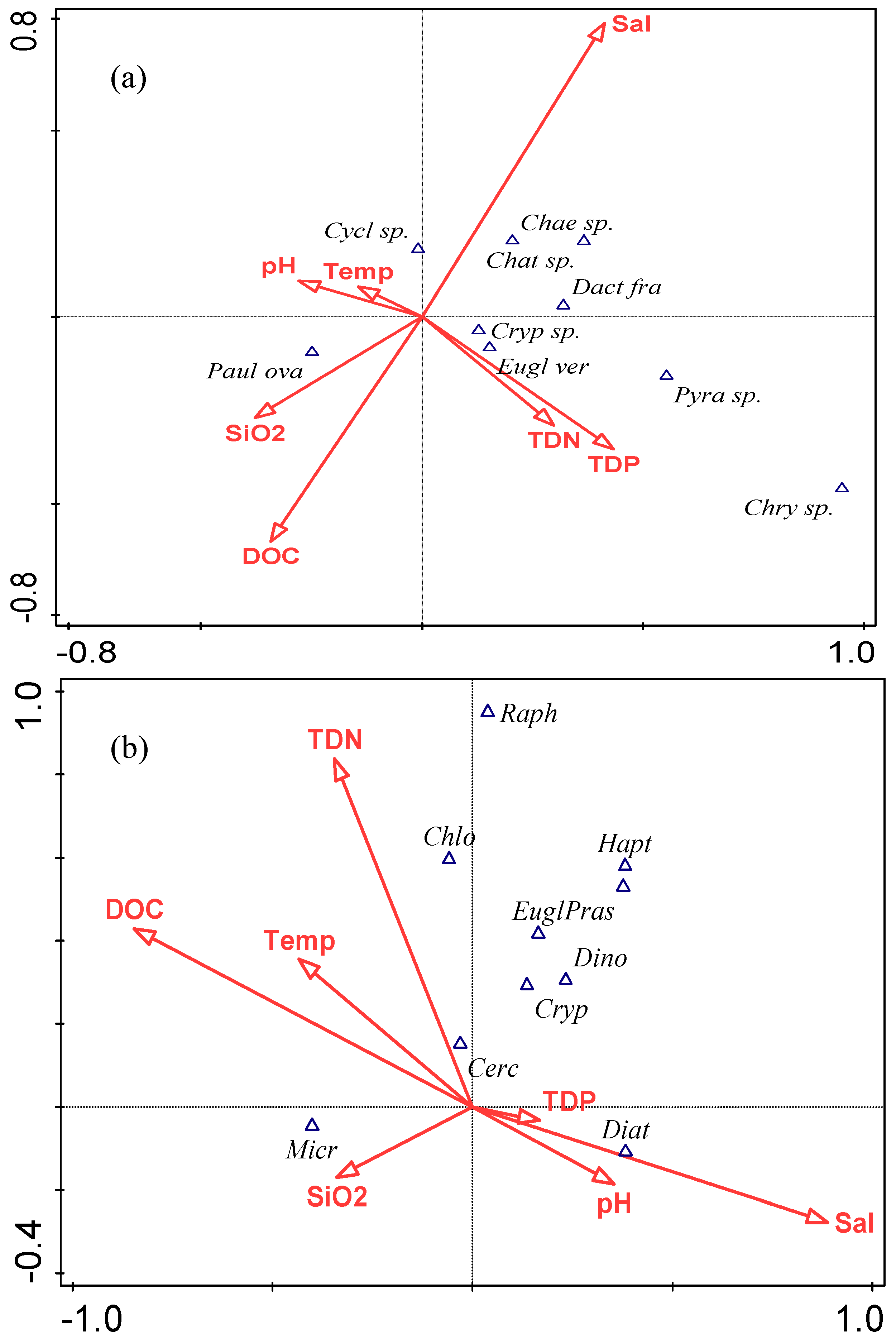
3.5. Relationships between Phytoplankton Assemblage based on Microscopic Counts and Physico-Chemical Variables

Most phytoplankton species and groups were strongly correlated to salinity, TDN or TDP (Figure 8a,b). The major diatom species (Chaetoceros sp. and D. fragilissimus) were negatively influenced by salinity, as highest mean densities were observed at Assawoman and Newport Bay sites (Figure 7a,c) with low salinities and relatively high freshwater input. Cyclotella sp. was most influenced positively by temperature (Figure 8a) as its peak density occurred in July (Figure 5b). This species was also the most dominant diatom species in that month. In addition, Cryptomonas sp. was associated with TDN and TDP. Other phytoplankton groups like raphidophytes, cercozoans, prasinophytes and chlorophytes did not show any significant correlations with the environmental parameters. Spatially, cryptophyte abundance and dissolved organic carbon (DOC) concentration followed the same pattern (Figure 9), being highest at site 6 (Newport Bay) and increasing from site 9 (Isle of Wight Bay) to site 13.

4. Discussion

This study addressed the seasonal and spatial variations in the composition of phytoplankton in the eutrophic northern and southern MCBs using a combination of photosynthetic pigments and microscopic counts. The results presented here give a more robust description of the phytoplankton community compared to results of previous phytoplankton studies in the Bays (e.g., [18,19,23,24,27]).

4.1. Phytoplankton Taxa Composition and Variation

A total of 40 phytoplankton genera comprising of 29 diatom, 6 dinoflagellate, 4 chlorophyte and 1 ochrophyte genera were observed which were not reported by previous investigators in the MCBs [18,19]. Dactyliosolen fragilissimus, Cyclotella sp. and Chaetoceros sp. were the dominant diatom species in the bays unlike in the lower section of Chesapeake Bay and northeastern coastal waters of the United States where the dominant diatoms were Skeletonema costatum, Leptocylindrus danicus and Asterionella glacialis [36,37,38]. In the western edges of Florida Bay, Hitchcock et al. [39] reported Dactyliosolen spp. and Chaetoceros spp. to be the most common diatoms. The high abundance of Cyclotella sp. in the MCBs [19] may be related to its tolerance for high salinity and various nutrient levels [40].

Fucoxanthin was the most abundant carotenoid pigment and among the fucoxanthin-containing algae, diatoms dominated the phytoplankton community as is typical of most coastal marine ecosystems in temperate areas [41,42,43]. Fucoxanthin was correlated with densities of diatoms, as well as with cercozoan abundance and the abundance of diatoms and cercozoans combined suggesting the presence of fucoxanthin containing cercozoans. Tamm et al. [44] attributed the good correlation between pigments and microscopic counts to “same species” dominance of phytoplankton community. Although fucoxanthin occurs mainly in diatoms, it is also present in chrysophytes [45].

Prorocentrum minimum, K. micrum, Gymnodinium sp. and Gyrodinium sp. were the most abundant dinoflagellates. These species in addition to other potentially harmful algal bloom forming dinoflagellate species such as D. acuminata and Alexandrium sp. were previously reported in the nearshore areas of MCBs and its tributaries [18,19]. Their occurrence especially in Newport Bay and the northern bay sites, located close to the mouths of tributaries, reflects the high nutrient levels that enter MCBs from tributaries and high water residence time that favors the accumulation of phytoplankton biomass. We observed bloom densities of the harmful algal species Heterocapsa rotundata in December in MCBs which had not been previously reported. Heterocapsa rotundata is a winter phytoplankton species [46], which blooms in stratified waters caused by high freshwater discharge events [47]. The high discharge in St. Martin River in October and December might have created such ideal conditions. Also, the high flow, low temperature (~14 °C) and the shallow nature of the Bays likely favored the disturbance of the sediment, providing cysts that acted as the bloom source [47]. Further studies are needed to investigate if there are variations with depth in phytoplankton and physico-chemical conditions at selected sites (particularly at the mouth of tributaries) in the bays, especially during periods of high freshwater discharge.

Only one haptophyte species was enumerated (Chrysochromulina sp.) and although Hex-fuco is the major carotenoid pigment [48] no correlation was observed between the pigment and Chrysochromulina sp. This could be attributed to the high variability in abundance of the species as it was observed mainly in late fall and winter and the fact that very small sized haptophytes might have been undercounted.

Cryptophytes were a major constituent (~10%) of the phytoplankton community and Cryptomonas sp., the dominant taxon, showed strong seasonal variability as did Allo. Traditionally, chlorophyll b and lutein have been used as indicators of green algae (chlorophytes) and MPF which lack external morphological features [32,49]. Chlorophytes, Euglenophytes and Prasinophytes contain Chl b [49] but no strong correlation was observed between the abundances of these classes and the pigment concentration.

Pyramimonas sp. was a dominant chlorophyte species and though prasinophytes have been reported as the dominant green algae in some marine areas [41], no correlation was observed between prasinophyte abundance and prasinoxanthin concentration. Schluter and Havskum [50] highlighted the connection between cell numbers and count reproducibility and emphasized that unlike in HPLC where large volumes of water are filtered, microscopy might fail to detect some phytoplankton cells in the small volume of water counted. In addition, Latasa et al. [51] reported the absence of Prasinoxanthin in certain strains of prasinophytes, especially the Pyramimonadales to which Pyramimonas sp. belongs. The MPF could have been responsible for the peak Chl b in July due to the strong correlation and similarity in pattern. In the tributaries of Assawoman Bay and St. Martin River of the MCBs, Tango et al. [18] previously reported the dominance of phytoflagellates in summer and fall.

4.2. Seasonal Patterns of Succession of Major Phytoplankton Taxa

The phytoplankton community in the winter was dominated by diatoms, with comparatively minor contributions from dinoflagellates and MPF. In spring and summer, the relative abundance of MPF and cercozoans increased and by early- to mid-fall, diatoms became abundant and were co-dominant with cryptophytes in November. These results are consistent with observations of phytoplankton dynamics in nutrient enriched estuaries and lagoons such as the Neuse River Estuary [46] and Indian River Lagoon [52]. Glibert et al. [23] reported that a shift in phytoplankton composition has occurred in the MCBs from dominance by microphytoplankton to dominance by picophytoplankton, particularly Aureococcus anophagefferens due to a long term increase in NH₄⁺ concentrations. In our study, MPF (mainly nanophytoplankton), cryptophytes and cercozoans increased in relative abundance in spring and summer while microphytoplankton relative abundance decreased. Furthermore, based on the concentration of A. anophagefferens biomarker pigment, But-fuco and the equation relating pigment concentration to cell numbers [20], over 9.1 × 10⁴ cells L⁻¹ were observed in June, corresponding to a Category 2 bloom and picoplanktonic cyanobacteria (represented by zeaxanthin) were most abundant in summer (June/July). The cyanobacteria were not identified to a generic level nor were they enumerated in this study because of their very small size. In a previous study, however, the cyanobacteria, Synechococcus spp. were observed in samples collected from MCBs (Chincoteague Bay) and their maximum density reached 1.3 × 10⁴ cells/mL in June [53].

4.3. Spatial Variation of Phytoplankton Abundance

The phytoplankton taxa composition and abundance varied spatially in the MCBs and this may be due to a number of factors including, land use characteristics of the watersheds, salinity, nutrient concentrations and retention due to differences in the rate of flushing of the bays [29]. The long residence time in the southern bays can cause nutrient and salinity variabilities, as have been reported in the Indian River Lagoon, IRL Florida [54]. In the IRL, watershed characteristics caused a potential phosphorus limitation indicated by high N:P ratios which impacted the phytoplankton community [55]. Similarly, in the MCBs very high TDN:TDP ratios were observed in the Isle of Wight and Newport Bay sites in April and October which could have caused the low biomass observed. Additionally, the unique characteristics of Newport Bay watershed (freshwater input, agricultural farms and wastewater treatment plant) provided conditions that favored the growth of a variety of diatom, cercozoan and cryptophyte species. In the IRL, low salinity sites were frequently dominated by dinoflagellates such as Prorocentrum sp. and Scrippsiella trochoidea [55], a pattern also evident in our study (data not shown) and corroborated by the CCA results.

Cryptophyte abundance and dissolved organic carbon (DOC) were strongly correlated and both variables followed a similar pattern spatially. In low light conditions, cryptophytes engulf bacteria and use organic matter as a carbon source [56]. Coincidentally, high cryptophyte densities occurred at sites (6, 10 and 13) which had high DOC concentrations from freshwater inputs and autochthonous production. It is likely that increased bacterial abundance and allochthonous organic matter input were responsible for the variability in cryptophyte abundance and positive relationship with DOC, especially at sites with high freshwater inputs [57].

Sites receiving relatively high freshwater inputs (6, 10, 11–13) had high biomass of phytoplankton, relatively low diatom abundance but comparatively high abundance of dinoflagellates and cercozoans. In spring and summer, the contribution of MPF (mainly nanophytoplankton) increased while microphytoplankton decreased, consistent with the reported long term increase in NH₄⁺ and subsequent shift in composition to nano- and picophytoplankton [23]. In the Galveston Bay estuary, Texas, nutrient loadings and nitrogen pulse events from freshwater discharge have resulted in differential responses of phytoplankton biomass and a shift from diatom dominance to cyanobacteria dominance or mixed assemblage in summer [58,59].

Other variables such as wind speed and direction, waves, tidal condition and solar radiation, that were not measured during the days samples were collected in this study, could possibly have also contributed to phytoplankton distribution in the bays. Due to the shallow nature of the lagoons, we expect that there is a close coupling between the pelagic and bottom parts of the bays as a result of wind and tidal action. This is more so in the fall and winter when wind speed is higher in the area than in the summer when wind speed is relatively low.

Spatial and seasonal differences in phytoplankton biomass contribute to variations in the transparency of the MCBs which is generally low. Nevertheless, enough light reaches the bottom of the bays in some areas to support benthic microalgae, seagrasses and macroalgae whose abundance has increased over the years, particularly in the northern bays. Transparency was lowest in the summer when phytoplankton biomass was highest and highest in fall when phytoplankton biomass was relatively low.

4.4. Dominance of Diatoms and Phosphorus Limitation

The dominance of diatoms in the coastal bays of Maryland revealed by both microscopic counts and HLPC pigment analysis is typical of most coastal marine systems [1,54,60]. Their highly efficient nutrient uptake and fucoxanthin content have been suggested to explain this dominance. Fucoxanthin is very efficient in absorbing green wavelength light, especially in coastal waters where dissolved and particulate organic matter may interfere with light in the green to yellow bands [61] thus giving fucoxanthin containing diatoms a competitive advantage over other species. Strong correlations were observed between fucoxanthin and diatoms during the study period. In April when a high TDN:TDP ratio was observed, inorganic phosphate was almost undetectable and TDP was very low, suggesting a severe phosphorus limitation. Coincidentally, low diatom cell densities and Chl a concentration were observed during the same period. Large eukaryotes such as diatoms do not thrive in phosphate depleted coastal waters [62]. Besides inorganic phosphate, diatom development may be inhibited by the lack of silica [63], although silica is not a limiting nutrient in the MCBs.

5. Conclusions

In the present study, the spatial and temporal variations in the phytoplankton composition and abundance were studied using photosynthetic pigments and microscopic counts. From findings of the study, the following can be concluded:

• Diatoms were the most abundant taxonomic group and showed strong correlations with its diagnostic pigment, fucoxanthin. There were also significant contributions from the nanophytoplankton especially in summer when they dominated the community, attributed largely to changes in nutrient composition and concentrations.
• Similar to other nutrient enriched estuaries along the US east coast, the MCBs displayed a distinct seasonal composition and variability in phytoplankton. Diatoms dominated the winter community while the relative abundance of the MPF and cercozoans increased, with diatoms and cryptophytes/cercozoans co-dominating in fall.
• Spatial variations in phytoplankton abundance and composition were likely due to environmental factors like watershed characteristics, nutrient levels and salinity. Sites receiving freshwater inputs directly from tributaries displayed high phytoplankton biomass.

The observed composition of phytoplankton species suggests that important changes have occurred in the phytoplankton assemblage that likely have affected the food web of these eutrophic bays. This information is valuable and underscores the need for continued efforts to implement measures aimed at reducing nutrient inputs into the bays. Further studies based on 18S rDNA are needed to enhance our knowledge of the phytoplankton assemblage and dynamics in the MCBs.

References

- Silva, A.; Mendes, C.R.; Palma, S.; Brotas, V. Short-time scale variation of phytoplankton succession in Lisbon bay (Portugal) as revealed by microscopy cell counts and HPLC pigment analysis. Estuar. Coast. Shelf Sci. 2008, 79, 230–238. [Google Scholar]
- Garmendia, M.; Borja, A.; Franco, J.; Revilla, M. Phytoplankton composition indicators for the assessment of eutrophication in marine waters: Present state and challenges within the European directives. Mar. Pollut. Bull. 2013, 66, 7–16. [Google Scholar] [CrossRef] [PubMed]
- Marshall, H.G. Phytoplankton of the York River. J. Coast. Res. 2009, 57, 59–65. [Google Scholar] [CrossRef]
- Glibert, P.M.; Wazniak, C.; Hall, M.; Sturgis, B. Seasonal and interannual trends in nitrogen in Maryland’s Coastal Bays and relationships with brown tide. Ecol. Appl. 2007, 17, S79–S87. [Google Scholar] [CrossRef]
- Gobler, C.J.; Sunda, W.G. Ecosystem disruptive algal blooms of the brown tide species Aureococcus anophagefferens and Aureoumbra lagunensis. Harmful Algae 2012, 14, 36–45. [Google Scholar] [CrossRef]
- Wilhelm, C.; Rudolf, I.; Renner, W. A quantitative method based on HPLC–aided pigment analysis to monitor structure and dynamics of the phytoplankton assemblage—A study from Lake Meerelder Mar (Eifel, Germany). Arch. Fur Hydrobiol. 1991, 123, 21–35. [Google Scholar]
- Domingues, R.B.; Barbosas, A.; Galvao, H. Constraints on the use of phytoplankton as a biological quality element within the Water Framework Directive in Portuguese waters. Mar. Pollut. Bull. 2008, 59, 1389–1395. [Google Scholar] [CrossRef] [PubMed]
- Harvey, H.W. Measurement of Phytoplankton Population. J Mar. Biol. Assoc. UK 1934, 19, 761–773. [Google Scholar] [CrossRef]
- Wright, S.W.; Jeffrey, S.W.; Mantoura, R.F.C.; Llewellyn, C.A.; Bjornland, T.; Repeta, D.; Welschmeyer, N. Improved HPLC method for the analysis of chlorophylls and carotenoids from marine phytoplankton. Mar. Ecol. Prog. Ser. 1991, 77, 183–196. [Google Scholar]
- Jeffrey, S.W.; Vesk, M. Introduction to marine phytoplankton and their pigment signatures. In Phytoplankton Pigments in Oceanography; Jeffrey, S.W., Mantoura, R.F.C., Wright, S.W., Eds.; UNESCO Publishing: Paris, France, 1997; pp. 37–84. [Google Scholar]
- Barlow, R.G.; Sessions, H.; Balarin, M.; Weeks, S.; Whittle, C.; Hutchings, L. Seasonal variation in phytoplankton in the southern Benguela: Pigment indices and ocean colour. Afr. J. Mar. Sci. 2005, 27, 275–288. [Google Scholar]
- Roy, R.; Pratihary, A.; Mangesh, G.; Naqvi, S.W.A. Spatial variation of phytoplankton pigments along the southwest coast of India. Estuar. Coast. Shelf Sci. 2006, 69, 189–195. [Google Scholar]
- Seoane, S.; Garmendia, M.; Revilla, M.; Borja, A.; Franco, J.; Orive, E.; Valencia, V. Phytoplankton pigments and epifluorescence microscopy as tools for ecological status assessment in coastal and estuarine waters, within the Water framework Directive. Mar. Pollut. Bull. 2011, 62, 1484–1497. [Google Scholar] [PubMed]
- Gieskes, W.W.C.; Kraay, G.W. Dominance of Cryptophyceae during the phytoplankton spring bloom in the central North Sea detected by HPLC analysis of pigments. Mar. Biol. 1983, 75, 179–185. [Google Scholar] [CrossRef]
- Wright, S.W.; Thomas, D.P.; Marchant, H.J.; Higgins, H.W.; Mackey, M.D.; Mackey, D.J. Analysis of phytoplankton of the Australian sector of the Southern Ocean: Comparisons of the microscopy and size frequency data with interpretations of pigment HPLC data using the ‘Chemtax’ matrix factorization program. Mar. Ecol. Prog. Ser. 1996, 144, 285–298. [Google Scholar] [CrossRef]
- Moreno, V.; Marrero, P.; Morales, J.; Llerandi García, C.; Villagarcía Úbed, M.D.; Rueda, M.J.; Llinás, O. Phytoplankton functional community structure in Argentinian continental shelf determined by HPLC pigment signatures. Estuar. Coast. Shelf Sci. 2012, 100, 72–81. [Google Scholar]
- Millie, D.F.; Schofield, O.M.; Kirkpatrick, G.J.; Johnsen, G.; Tester, P.A.; Vinyard, B.T. Detection of harmful algal blooms using photopigments and absorption signatures: A case study of the Florida red tide dinoflagellate, Gymnodinium breve. Limnol. Oceanogr. 1997, 42, 1240–1251. [Google Scholar] [CrossRef]
- Tango, P.; Butler, W.; Wazniak, C. Assessment of Harmful algal bloom species in the Maryland Coastal Bays. In Maryland’s Coastal Bays: Ecosystem Health Assessment; Chapter 7.2; Maryland Department of Natural Resources, Tidewater Ecosystem Assessment: Annapolis, MD, USA, 2004; pp. 11–27. [Google Scholar]
- Tango, P.; Butler, W.; Wazniak, C. Analysis of phytoplankton populations in the Maryland Coastal Bays. In Maryland’s Coastal Bays: Ecosystem Health Assessment; Chapter 8.1; Maryland Department of Natural Resources, Tidewater Ecosystem Assessment: Annapolis, MD, USA, 2004; pp. 2–34. [Google Scholar]
- Trice, T.M.; Gilbert, P.M.; Van Heukelem, L. HPLC pigment records provide evidence of past blooms of Aureococcus anophagefferens in the coastal bays of Maryland and Virginia, USA. Harmful Algae 2004, 3, 295–304. [Google Scholar]
- Wazniak, C.E.; Hall, M.R.; Carruthers, T.J.; Sturgis, B.; Dennison, W.C.; Orth, R.J. Linking water quality to living resources in a Mid-Atlantic lagoon system, USA. Ecol. Appl. 2007, 17, S64–S78. [Google Scholar] [CrossRef]
- Fertig, B.; O’Neil, J.M.; Beckert, K.A.; Cain, C.J.; Needham, D.M.; Carruthers, T.J.B.; Dennison, W. Elucidating terrestrial nutrient sources to a coastal lagoon, Chincoteague Bay, Maryland USA. Estuar. Coast. Shelf Sci. 2013, 116, 1–10. [Google Scholar] [CrossRef]
- Glibert, P.M.; Hinkle, D.C.; Sturgis, B.; Jesien, R.V. Eutrophication of a Maryland/Virginia Coastal Lagoon: A tipping point, ecosystem changes, and potential causes. Estuar. Coasts 2014, 37, 128–146. [Google Scholar]
- Oseji, O.F.; Chigbu, P.; Oghenekaro, E.; Waguespack, Y.; Chen, N. Spatial and temporal patterns of phytoplankton composition and abundance in the Maryland Coastal Bays: The influence of freshwater discharge and anthropogenic activities. Estuar. Coast. Shelf Sci. 2018, 207, 119–131. [Google Scholar] [CrossRef]
- Duan, S.; Chen, N.; Kaushal, S.; Chigbu, P.; Ishaque, A.; May, E.B.; Oseji, O.F. Dynamics of dissolved organic carbon and nitrogen in the Maryland Coastal Bays. Estuar. Coast. Shelf Sci. 2015, 164, 451–462. [Google Scholar] [CrossRef]
- Mulholland, M.R.; Boneillo, G.E.; Bernhardt, P.W.; Minor, E.C. Comparison of nutrient and microbial dynamics over a seasonal cycle in a Mid-Atlantic Coastal lagoon prone to Aureococcus anophagefferens (Brown Tide) blooms. Estuar. Coasts 2009, 32, 1176–1194. [Google Scholar] [CrossRef]
- Boynton, W.R.; Hagy, J.D.; Murray, L.; Stokes, C. A comparative analysis of eutrophication patterns in a temperate coastal Lagoon. Estuaries 1996, 19, 408–421. [Google Scholar] [CrossRef]
- Wazniak, C.; Hall, M.; Cain, C.; Wilson, D.; Jesien, R.; Thomas, J.; Carruthers, T.; Dennison, W. State of the Maryland Coastal Bays; A Report; Maryland Coastal Bays Program: Berlin, MD, USA, 2004; 44p. [Google Scholar]
- Pritchard, D.W. Salt balance and exchange rate for Chincoteague Bay. Chesap. Sci. 1960, 1, 48–57. [Google Scholar] [CrossRef]
- Bratton, J.F.; Bohlke, J.K.; Krantz, D.E.; Tobias, C.R. Flow and geochemistry of groundwater beneath a back-barrier lagoon: The subterranean estuary at Chincoteague Bay Maryland, USA. Mar. Chem. 2009, 113, 78–92. [Google Scholar] [CrossRef]
- Kennish, M.J.; Paerl, H.W. Coastal Lagoons: Critical Habitats of Environmental Change; CRC Press: Boca Raton, FL, USA, 2010; 568p. [Google Scholar]
- Jeffrey, S.W.; Wright, S.W. Qualitative and Quantitative Analysis of SCOR Reference Algal Cultures. In Phytoplankton Pigments in Oceanography: Guidelines to Modern Methods; Jeffrey, S.W., Mantoura, R.F.C., Wright, S.W., Eds.; UNESCO: Paris, France, 1997; pp. 343–360. ISBN 92-3-103275-5. [Google Scholar]
- Chen, J.; Oseji, O.; Mitra, M.; Waguespack, Y.; Chen, N. Phytoplankton pigments in Maryland Coastal Bay sediments as biomarkers of sources of organic matter to benthic Community. J. Coast. Res. 2015, 32, 768–775. [Google Scholar] [CrossRef]
- Zapata, M.; Rodríguez, F.; Garrido, J.L. Separation of chlorophylls and carotenoids from marine phytoplankton: A new HPLC method using a reversed phase C8 column and pyridine containing mobile phases. Mar. Ecol. Prog. Ser. 2000, 195, 29–45. [Google Scholar] [CrossRef]
- Ter Braak, C.J.F.; Smilauer, P. CANOCO Reference Manual and CanoDraw for Windows User’s Guide: Software for Canonical Community Ordination (Version 4.5); Biometris Wageningen: Wageningen, The Netherlands, 2002. [Google Scholar]
- Marshall, H.G. The composition of phytoplankton within the Chesapeake Bay plume and adjacent waters off the Virginia coast, U.S.A. Estuar. Coast. Shelf Sci. 1982, 5, 29–43. [Google Scholar] [CrossRef]
- Marshall, H.G.; Cohn, M.S. Distribution and composition of phytoplankton in northeastern coastal waters of the United States. Estuar. Coast. Shelf Sci. 1983, 17, 119–131. [Google Scholar] [CrossRef]
- Marshall, H.G.; Lacouture, R. Seasonal patterns of growth and composition of phytoplankton in the lower Chesapeake Bay and vicinity. Estuar. Coast. Shelf Sci. 1986, 23, 115–130. [Google Scholar]
- Hitchcock, G.; Phlips, E.; Brand, L.; Morrison, D. Plankton Blooms. In Florida Bay Science Program: A Synthesis of Research on Florida Bay; Fish and Wildlife Research Institute Technical Report TR-11; Hunt, J.H., Nuttle, W., Eds.; Florida Fish and Wildlife Research Institute: St Petersburg, FL, USA, 2007; pp. 77–91. [Google Scholar]
- Trigueros, J.M.; Ansotegui, A.; Orive, E.; Nó, M.L. Morphology and distribution of two brackish diatoms (Bacillariophyceae): Cyclotella atomus Hustedt and Thalassiosira guillardii Hasle in the estuary of Urdaibai (northern Spain). Nova Hedwig. 2000, 70, 431–450. [Google Scholar]
- Lohrenz, S.E.; Carroll, C.L.; Weidemann, A.D.; Tuel, M. Variations in phytoplankton pigments, size structure and community composition related to wind forcing and water mass properties on the North Carolina inner shelf. Cont. Shelf Res. 2003, 23, 1447–1464. [Google Scholar]
- Rodrı’guez, F.; Pazos, Y.; Maneiro, J.; Zapata, M. Temporal variation in phytoplankton assemblages and pigment composition at a fixed station of the Ria of Pontevedra (NW Spain). Estuar. Coast. Shelf Sci. 2003, 58, 499–515. [Google Scholar] [CrossRef]
- Litchman, E.; Klausmeier, C.A.; Yoshiyama, K. Contrasting size evolution in marine and freshwater diatoms. Proc. Natl. Acad. Sci. USA 2009, 106, 2665–2670. [Google Scholar] [CrossRef] [PubMed] [Green Version]
- Tamm, M.; Freiberg, R.; Tõnno, I.; Nõges, P.; Nõges, T. Pigment-Based Chemotaxonomy—A quick alternative to determine algal assemblages in large shallow eutrophic Lake? PLoS ONE 2015, 10, e0122526. [Google Scholar] [CrossRef]
- Seoane, S.; Laza-Martinez, A.; Orive, E. Monitoring phytoplankton assemblages in estuarine waters: The application of pigment analysis and microscopy to size-fractionated samples. Estuar. Coast. Shelf Sci. 2006, 67, 343–354. [Google Scholar] [CrossRef]
- Mallin, M. Phytoplankton ecology of North Carolina estuaries. Estuaries 1994, 17, 561–574. [Google Scholar] [CrossRef]
- Cohen, R.R.H. Physical processes and the ecology of a winter dinoflagellate bloom of Katodinium rotundatum. Mar. Ecol. Prog. Ser. 1985, 26, 135–144. [Google Scholar]
- Johnsen, G.; Sakshaug, E.; Vernet, M. Pigment composition, spectral characterization and photosynthetic parameters in Chrysochromulina polylepis. Mar. Ecol. Prog. Ser. 1992, 83, 241–249. [Google Scholar]
- Roy, S.; Llewellyn, C.A.; Egeland, E.S.; Johnsen, G. Phytoplankton Pigments: Characterization, Chemotaxonomy and Applications in Oceanography; Cambridge University Press: Cambridge, UK, 2012; 845p. [Google Scholar]
- Schluter, L.; Havskum, H. Phytoplankton pigments in relation to carbon content in phytoplankton communities. Mar. Ecol. Prog. Ser. 1997, 155, 55–65. [Google Scholar] [CrossRef] [Green Version]
- Latasa, M.; Scharek, R.; Le Gall, F.; Guillou, L. Pigment suites and taxonomic groups in Prasinophyceae. J. Phycol. 2004, 40, 1149–1155. [Google Scholar] [CrossRef]
- Phlips, E.J.; Badylak, S.; Christman, M.C.; Lasi, M.A. Climatic trends and temporal patterns of phytoplankton composition, abundance and succession in the Indian River Lagoon, Florida, USA. Estuar. Coasts 2010, 33, 498–512. [Google Scholar] [CrossRef]
- Deonarine, S.N.; Gobler, C.J.; Lonsdale, D.J.; Caron, D.A. Role of zooplankton in the onset and demise of harmful brown tide blooms (Aureococcus anophagefferens) in US mid-Atlantic estuaries. Aquat. Microb. Ecol. 2006, 4, 181–195. [Google Scholar] [CrossRef]
- Badylak, S.; Phlips, E.J. Spatial and temporal patterns of phytoplankton composition in a subtropical coastal lagoon, the Indian River Lagoon, Florida, USA. J. Plankton Res. 2004, 26, 1229–1247. [Google Scholar] [CrossRef]
- Phlips, E.J.; Badylak, S.; Grosskopf, T. Factors affecting the abundance of phytoplankton in a restricted sub-tropical lagoon, the Indian River Lagoon, Florida, USA. Estuar. Coast. Shelf Sci. 2002, 55, 385–402. [Google Scholar] [CrossRef]
- Bellinger, E.G.; Sigee, D.C. Freshwater Algae: Identification and Use as Bioindicators; John Wiley and Sons: Oxford, UK, 2010; 265p. [Google Scholar]
- Abirhire, O.; North, R.L.; Hunter, K.; Vandergutch, D.; Sereda, J.; Hudson, J. Environmental factors influencing phytoplankton communities in Lake Diefenbaker, Saskatchewan, Canada. J. Great Lakes Res. 2015, 41, 118–128. [Google Scholar] [CrossRef]
- Örnólfsdóttir, E.B.; Lumsden, S.E.; Pinckney, J.L. Nutrient pulsing as a regulator of phytoplankton abundance and community composition in Galveston Bay, Texas. J. Exp. Mar. Biol. Ecol. 2004, 303, 197–220. [Google Scholar] [CrossRef]
- Dorado, S.; Booe, J.; Steichen, J.; McInnes, A.; Windham, R.; Shepard, A.; Lucchese, A.; Preischel, H.; Pinckney, J.L.; Davis, S.; et al. Towards an understanding of the interactions between freshwater inflows and phytoplankton communities in a subtropical estuary in the Gulf of Mexico. Public Libr. Sci. One 2015, 10, e0130931. [Google Scholar] [CrossRef] [PubMed]
- Gin, K.Y.H.; Zhang, S.; Lee, Y.K. Phytoplankton community structure in Singapore’s coastal waters using HPLC pigment analysis and flow cytometry. J. Plankton Res. 2003, 25, 1507–1519. [Google Scholar] [CrossRef]
- Ondrusek, M.E.; Bidigare, R.R.; Sweet, S.T.; Defreitas, D.A.; Brooks, J.M. Distribution of phytoplankton pigments in the North Pacific Ocean in relation to physical and optical variability. Deep Sea Res. 1991, 38, 243–266. [Google Scholar] [CrossRef]
- Donald, K.M.; Scanlan, D.J.; Carr, N.G.; Mann, N.H.; Joint, I. Comparative phosphorus nutrition of the marine cyanobacterium Synechococcus WH7803 and the marine diatom Thalassiosira weissflogii. J. Plankton Res. 1997, 19, 1793–1813. [Google Scholar] [CrossRef]
- Cloern, J.E.; Dufford, R. Phytoplankton community ecology: Principles applied in San Francisco Bay. Mar. Ecol. Prog. Ser. 2005, 285, 11–28. [Google Scholar] [CrossRef]
Figure 1.
Map of the Maryland Coastal Bays showing the 13 stations where samples were collected for nutrients, phytoplankton counts and pigment analyses.
Figure 2.
Monthly variations of surface temperature (a), salinity (ppt) (b), pH (c) and stream flow from the Birch Branch gauge in cubic meters per second (d) during the sampling period (February and December 2012).
Figure 3.
Mean monthly variation of dissolved organic carbon (a), total dissolved nitrogen (b), total dissolved phosphorus (c), silica (d) at the sampling sites grouped by embayment, TDN:TDP (e) and Si:TDN (f) ratios during the sampling period (February and December 2012). Sites 1–5, 6, sites 7–8, 9, 10 and sites 11–13 are located in Chincoteague Bay, Newport Bay, Sinepuxent Bay, Isle of Wight Bay, St. Martin River and Assawoman Bay, respectively. The dashed colored lines represent missing data. The dashed black line represents the Redfield TDN:TDP threshold of 45, (e) and the Si:TDN threshold of 1 (f).
Figure 4.
Temporal variations of phytoplankton groups and their photosynthetic pigment biomarkers (a–k).
Figure 5.
The seasonal variation in the relative abundance of major phytoplankton taxa (a) and temporal variation of the most abundant diatom taxa in the MCBs; Dactyliosolen fragilissimus, Cyclotella sp. and Chaetoceros sp. (b). Diat-diatoms, Crypt-Cryptophytes, Cerc-Cercozoans, MPF-Microphytoflagellates, Dino-Dinoflagellates, Others-all other phytoplankton classes.
Figure 6.
Spatial variation of the relative abundance of major phytoplankton taxonomic groups in winter (a), spring (b), summer (c) and fall (d) at each embayment of the MCBs. In each plot, Diat-diatoms, Crypt-Cryptophytes, Cerc-Cercozoans, MPF-Microphytoflagellates, Dino-Dinoflagellates, Others-all other phytoplankton classes.
Figure 7.
Spatial distribution of the most abundant phytoplankton species belonging to the major taxa found in the assemblage, including diatoms (a–c), cryptophytes (d), cercozoans (e), euglenozoans (f), haptophytes (g), chlorophytes (h) and ochrophytes (i).
Figure 8.
Canonical correspondence analysis (CCA) biplots of phytoplankton species (a) and major groups (b). Key: solid arrows represent environmental variables; Cycl sp.-Cyclotella sp., Chae sp.-Chaetoceros sp., Chat sp.-Chattonella sp., Dact fra-Dactyliosolen fragilissimus, Cryp sp.-Cryptomonas sp., Eugl ver-Euglena veridis, Paul ova-Paulinella ovalis, Pyra sp.-Pyramimonas sp., Chry sp.-Chrysochromulina sp., Chlo-Chlorophytes, Raph-Raphidophytes, Hapt-Haptophytes, Eugl-Euglenozoans, Pras-Prasinophytes, Dino-Dinoflagellates, Cryp-Cryptophytes, Cerc-Cercozoans, Diat-Diatoms, Micr-Microphytoflagellates.
Figure 9.
Spatial relationship between cryptophyte abundance obtained from microscopic counts and dissolved organic carbon (DOC).