Isohyetal Maps of Daily Maximum Rainfall for Different Return Periods for the Colombian Caribbean Region

Abstract

In Colombia, daily maximum multiannual series are one of the main inputs for design streamflow calculation, which requires performing a rainfall frequency analysis that involves several prior steps: (a) requesting the datasets, (b) waiting for the information, (c) reviewing the datasets received for missing or data different from the requested variable, and (d) requesting the information once again if it is not correct. To tackle these setbacks, 318 rain gauges located in the Colombian Caribbean region were used to first evaluate whether or not the Gumbel distribution was indeed the most suitable by performing frequency analyses using three different distributions (Gumbel, Generalized Extreme Value (GEV), and Log-Pearson 3 (LP3)); secondly, to generate daily maximum isohyetal maps for return periods of 2, 5, 10, 20, 25, 50, and 100 years; and, lastly, to evaluate which interpolation method (IDW, spline, and ordinary kriging) works best in areas with a varying density of data points. GEV was most suitable in 47.2% of the rain gauges, while Gumbel, in spite of being widely used in Colombia, was only suitable in 34.3% of the cases. Regarding the interpolation method, better isohyetals were obtained with the IDW method. In general, the areal maximum daily rainfall estimated showed good agreement when compared to the true values.

1. Introduction

Designing hydraulic structures for stormwater management encompasses several tasks, among which are: (a) watershed morphometric analysis, (b) estimation of the time of concentration, (c) calculation of the design rainfall via frequency analysis (typically, under stationary conditions), (d) design flow computation, (e) sizing the hydraulic structure per se, and (f) hydraulic modeling to evaluate the structure’s hydraulic performance under various return periods. The design flow may be estimated via either a rainfall-runoff model or regression equations (in ungauged watersheds), or stationary frequency analysis of streamflow data, if available.

Unlike streamflow data, rainfall observations are the most abundant hydrometeorological variable available. Rainfall observations, as a result, are most commonly used when estimating the flow value in ungauged watersheds (via rainfall-runoff models) to design hydraulic structures for runoff management. The Institute of Hydrology, Meteorology, and Environmental Studies of Colombia (IDEAM in Spanish) has hundreds of rain gauges (pluviometers and pluviographs) within Colombia. However, there are certain limitations when it comes to the availability of the rainfall data. The most common are: areas not covered due to either the absence of a rain gauge, or rain gauges no longer in service, or the rain gauges are mostly pluviometers (not pluviographs). The latter limits the ability to: (a) try to understand the real (measured) rainfall’s behavior during a day (its temporal distribution) and (b) derive, for instance, Intensity-Duration-Frequency (IDF) curves directly from registered time increments of daily rainfall (from pluviographs). Instead, synthetic IDF curves are typically derived [1,2,3], which often need multiannual 24-h maximum rainfall (P_24h-max) as one of the main inputs to later estimate the rainfall (intensity) value associated with a selected return period: the design rainfall.

IDEAM has lately made many efforts in compiling the majority of the hydrometeorological information freely available for all. The amount of analyzed information on record has considerably increased in the last decade. For instance, total annual average rainfall and temperature were modeled via regional climate models to try to quantify their behavior over the years 2011–2100 by taking into account climate change [4]. Furthermore, during the years 2015 and 2016, IDEAM updated the Intensity-Duration-Frequency (IDF) curves of 130 rain gauges (only 14 of them were in the Caribbean region) by using pluviographs with rainfall observations up to 2010 [5]. On the other hand, MinVivienda [6] recently mandated to both utilize updated rainfall observations that include data of the last five years on record and evaluate the influence of climate change on the rainfall pattern of the area of interest whenever a stormwater system is to be designed. It also recommends to check regularly for the bulletins IDEAM issues (and updates) on climate change and the influence on rainfall. All this represents, undoubtedly, a significant step towards a better understanding (and analysis) of the hydrometeorological variables and their use either in the design of stormwater systems or watershed management plans. Nonetheless, there is information still waiting to be processed, analyzed, and presented in different formats. Because of this, hydrologists and other water-related professionals and scientists sometimes spend a considerable amount of time on rainfall analyses. For frequency analysis, multiple probability functions with two and/or three parameters have been developed to fit the extreme data, among which are: Gumbel, log-normal, gamma, exponential, Pearson 3 (P3), Log-Pearson 3 (LP3), and Generalized Extreme Value (GEV) [1,2]. The variable analyzed is considered both random and independent [1,2]. Some countries have opted to officially recommend the use of one probability distribution function so as to unify criteria. Several studies have been conducted in order to improve the results obtained from frequency analysis. Li et al. [7] and Chowdhury et al. [8] assessed the performance of various distributions (gamma, exponential, mixed-exponential, log-normal) and proposed enhancements by means of stochastic models. Furthermore, regional studies have utilized different probability distribution functions to analyze rainfall data. Pizarro et al. [9] developed a web-based platform to develop IDF curves in Chile by using three distribution functions (Gumbel, GEV, and P3). Burgess et al. [10] updated the existing IDF curves of Jamaica by means of a frequency analysis under the Gumbel distribution. Seo et al. [11] derived design rainfall values via Gumbel and GEV distributions, and the parameter estimation was made through the minimum density power divergence estimator. Nguyen and Nguyen [12] developed a tool to evaluate the performance of ten probability distributions (beta-K, beta-P, GEV, generalized logistic, generalized normal, generalized Pareto, Gumbel, LP3, P3, and Wakeby) over rainfall data in Ontario (Canada). Likewise, isohyetal maps for different durations for various countries have been developed using various probability functions to fit the datasets [13,14,15,16,17]. Independently of the probability distribution function used to derive the isohyetals, having a map, where the design rainfall values for different return periods can be easily selected, would both substantially reduce the time dedicated to this activity and help with the estimation of design rainfalls, especially in ungauged areas, necessary for projects and studies (both local and foreign) with a hydrological and hydraulic component such as flood risk evaluation and mitigation, environmental impact assessments, land development, stream restoration, and the design of hydraulic structures for stormwater management. Unfortunately, there is no such map in Colombia. The lack of readily-available and processed information might become an obstacle in the understanding and development of these projects. Furthermore, in the absence of data, detailed isohyetal maps such as the ones developed in this research can be utilized for both regional and global analyses of extreme rainfall event proxies, hydrological regime changes, climate studies, water balance estimation under various scenarios, and the development of water management strategies.

This study intends to contribute to these tasks by: (a) first carrying out rainfall stationary frequency analyses by means of three different Cumulative Distribution Functions (CDF) for extreme values analysis (Gumbel, GEV, and LP3) so as to confirm whether or not the Gumbel distribution is indeed the most suitable for the rainfall data of this study, as it is the most commonly used in Colombia despite the fact that the other two have been also assessed in various studies [18,19,20,21,22,23]; (b) secondly, evaluating which spatial interpolation method is most suitable given the highly-dense spatial distribution of the rain gauges; and (c) lastly, drawing isohyetal maps of P_24h-max—via Geographical Information System (GIS)—for return periods of 2, 5, 10, 20, 25, 50, and 100 years for the Colombian Caribbean region as the first step in a more ambitious project of elaborating maps for the remaining regions (Pacific, Andean, Orinoco, and Amazon). For that, 318 pluviometric stations (rain gauges) operated by IDEAM—with at least 30 years of data—were used. The rain gauges are distributed as follows: 313 throughout the seven departments that compose the Colombian Caribbean region (Guajira, Magdalena, Cesar, Atlántico, Bolívar, Sucre, and Córdoba) and five from neighboring departments (Antioquia, Santander, and Norte de Santander).

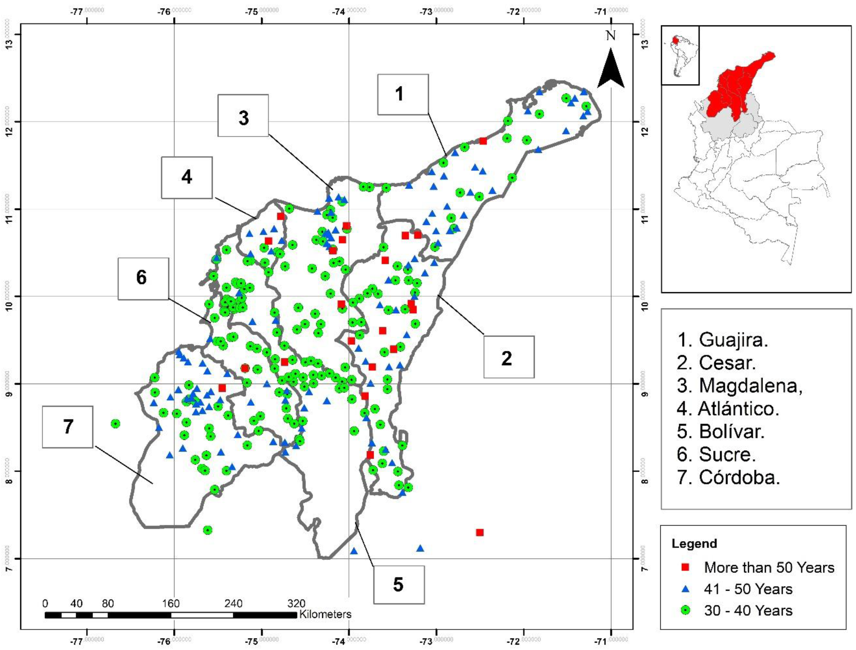
2. Study Area and Data

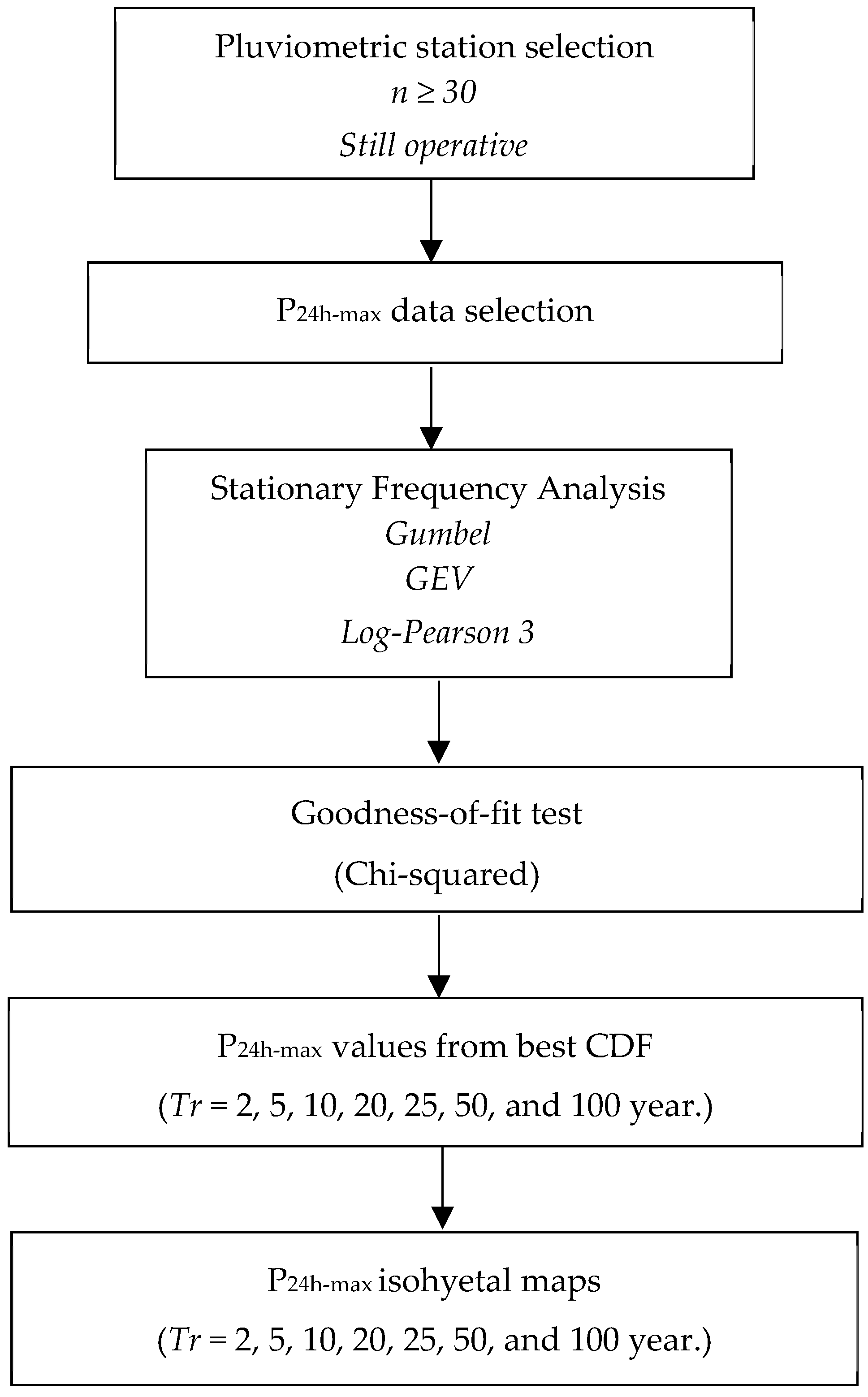
The Caribbean region of Colombia is comprised of seven political and administrative territorial units (called departments), namely Guajira, Magdalena, Cesar, Atlántico, Bolívar, Sucre, and Córdoba, which sum up a total area of 132,244 km² (accounting for approximately 0.012% of the country’s total surface area). It has an average annual precipitation that ranges from 0–1500 mm (the region’s northern portion) and from 1500 mm up to 5000 mm (in some areas of the southern portion of the departments of Bolívar and Córdoba) [4]. The region is mostly composed of plains, with the exception of the mountain ranges of San Jacinto (located within the departments of Sucre and Bolívar) and Santa Marta (department of Magdalena). The rainiest departments are Bolívar and Sucre, while the driest is Guajira. The average annual temperature is about 30 °C with some areas where it may increase or decrease depending on the climatological season and altitude. The rainfall climate regime of the Colombian Caribbean region has three seasons [24]: dry (December–March), transition—also known as Veranillo de San Juan—(June–July), and rainy (April–June and August–November). The duration of these seasons is affected by the El Niño Southern Oscillation (ENSO) phenomenon [25,26,27,28,29].

The data used in this study correspond to multiannual series of P_24h-max that include a total of 12,828 observations till the year 2015 from 318 pluviometric stations (the oldest station in this study started to operate in 1931). Years 2016 and 2017 were not included because the data from some of the stations have not been officially released by IDEAM. The pluviometric stations selected had to comply with the following criteria: (a) being still operative and (b) having at least 30 years of observations [30]. Additionally, P_24h-max values were eliminated if they came from a year not having a minimum of 150 days of data [31,32,33] and/or missing any of the months of the rainy season. The resulting rainfall data are summarized in

Table 1. Summary of rainfall data analyzed.

Department	No. of Rain Gauges	Total P24h-max Observations	P24h-max Value (mm)			Year of Installation of the Oldest Rain Gauge
			Max	Min	Avg.
Guajira	44	1834	247.6	5.4	77.6	1937
Cesar	60	2478	271.0	20.0	99.8	1931
Magdalena	55	2159	267.0	15.0	98.7	1956
Atlántico	13	568	250.0	30.0	83.8	1941
Bolívar	57	2153	280.0	24.5	104.4	1941
Sucre	32	1232	301.0	32.0	101.9	1945
Córdoba	53	2184	250.0	34.0	96.4	1959
Antioquia	3	115	254.0	54.0	106.4	1974
Santander	1	61	100.0	20.0	45.48	1956
Norte de Santander	1	44	152.0	38.4	77.0	1974
Total	318	12,828

Gray cells indicate the maximum and minimum values (of all) recorded, respectively.

. Figure 1 shows the departments and the geographical location of the rain gauges. Out of the 318 rain gauges, 183 have 30–40 years of data, 113 have 41–50 years of data, and 22 have more than 50 years of rainfall observations. It may also be observed that the southern areas of the departments of Bolívar and Córdoba have no rain gauges that fit the selection criteria. To fill these gaps, it is necessary to improve the isohyetal alignment, so five additional rain gauges were used. The rain gauges are located within the three neighboring departments of Antioquia (three rain gauges), Santander (one rain gauge), and Norte de Santander (one rain gauge). Despite the fact that these three departments do not belong to the Caribbean region, the rain gauges selected are located close to the southern portion of the Caribbean region.

Table 2. Rain gauges of the area of study.

Dept.	Rain Gauge Name
Atlántico	Hibaracho, Lena, Polo Nuevo, Puerto (Pto.) Giraldo, Casa de Bombas, Repelón, Sabanalarga, Los Campanos, Hacienda (Hda.) El Rabón, Aeropuerto (Apto.) Ernesto Cortissoz, Ponedera, San Pedrito Alerta, and Usiacurí.
Bolívar	Bayunca, Apto. Rafael Núñez, Escuela Naval-Centro de Investigaciones Oceanográficas e Hidrográficas (CIOH), Santa (Sta.) Ana, Guacamayo, Guaranda, Buenavista, Rionuevo, Arenal, Arjona, Rocha, Sincerín, Barranco Loba, El Limón, La Esperanza, Córdoba, Carmen de Bolívar, Camarón, Pozón, Aguadas La Alerta, San Antonio, Barraco Yuca, Coyongal Alertas, Barbosa, Baracoa, Gamero, San Basilio, El Viso, Chilloa, Flamenco, La Calma, Níspero, Plátano, Mampuján, Presa Arroyo Grande, Nueva Florida, San Pablo, Sta. Cruz, Candelaria, Guaymaral, Mompox, Pinillos, Regidor, San Estanislao, Sta. Rosa, El Jolón, San Cristobal, Casa Piedra, Caimital, La Candelaria, Astilleros, La Raya, San Cayetano, Playitas, Zambrano, Hda. Indugan, and Cañaveral.
Cesar	Villa Marlene, Patillal, Atanquez, París de Francia, La Esperanza, Caracolí, San Ángel, Villa Rosa, El Callao, Apto. Alfonso López, Guaymaral, Barranca Lebrija, Totumal, Aguas Claras, Hda. Las Playas, Hda. Sta. Teresa, Codazzi del Cesar (DC), Hda. Centenario, El Retorno, Motilonia Codazzi, Astrea, El Yucal, Socomba, Bosconia, Palmariguaní, Hda. Manature, El Canal, Saloa, Hda. El Terror, Chimichagua, Rincón Hondo, Chiriguaná, Curumaní, Zapatoza, Poponte, La Primavera, La Loma, El Paso, Puerto Mosquito, Gamarra, La Gloria, La Vega, La Jagua, Manaure, La Raya, Sta. Isabel, Pueblo Bello, San Sebastián de Rábago, Río de Oro, Los Ángeles, Hda. San Daniel, El Líbano, San Alberto, Los Planes, San Benito, San Gabriel, Leticia, El Rincón, La Dorada, and Tamalameque.
Córdoba	Sta. Lucía, Hda. Sta. Cruz, Loma Verde, Galán, San Anterito, Buenos Aires, Maracayo, Boca de la Ceiba, Sabanal, Universidad de Córdoba, Apto. Los Garzones, Los Pájaros, Cecilia, Ayapel, Buenavista, Rabolargo, Canalete, Cereté, Turipana, Chimá, Chinú, Turipana, El Salado, La Apartada, La Doctrina, Lorica, Momil, Pica Pica, San Francisco, Hda. Cuba, Centro Alegre, Planeta Rica, Cintura, Hda. Sajondía, Jaramagal, Cristo Rey, Hda. Las Acacias, Sahagún, Jobo El Tablón, Trementino, Colomboy, El Limón, San Bernardo del Viento, San Carlos, Sta. Rosa, Carrizal, Callemar, Corozal 2, San Antonio, Carrillo, Uré, Tierra Alta, and Carmelo.
Guajira	Matitas, Camarones, Los Remedios, Apto. Almirante Padilla, La Arena, Cuestecita, Hda. La Esperanza, Lagunitas, Sabanas de Manuela, Dibulla, Las Lomitas, El Juguete, El Conejo, La Paulina, Escuela Ceura, Paraguachón, Escuela Agropecuaria Carraipía, El Pájaro, Mayapo, Caracas, Manaure, Cañaverales, Hatico de los Indios, San Juan del Cesar, Santana Urraich, Nuevo Ambiente, Buenos Aires, Kauraquimaná, Irraipa, Perpana, Carrizal, Jojoncito, Caimito, Puerto Estrella, Orochón, Sipanao, Siapana, Sillamaná, Jasay, Puerto López, Nazareth, Rancho Grande, Urumita, and Villanueva.
Magdalena	Vista Nieves, Buritaca, Minca, Apto. Simón Bolívar, Guacacha, San Lorenzo, Palomino, Cenizo, La María, Villa Concepción, Campamento El Difícil, Hda. La Cabaña, San Pablo, La Ye, La Palma, Menchiquejo, El Palmor, Sevillano, San Roque, Tiogollo, Negritos, Las Flores, El Bongo, El Destino, Gavilán, La Florida, Bellavista, Bayano, Fundación Rosa de Lima, Nueva Granada, Irán, Doña María, Monterrubio, Garrapata, Apure El Agrado, Tasajera, La Esperanza, Palo Alto, San Rafael, San Ángel, San Sebastián, Salamina, San Zenón, El Brillante, Tierra Grata, La Mecha, El Pueblito, Los Cocos, El Carmen, El Enano, Prado Sevilla, Los Proyectos, and La Unión.
Sucre	Hda. La Frontera, Caimito, Primates, Hato Nuevo, Apto. Rafael Bravo, Galeras, Villanueva, Pto. Asis, Palmarito, Zapata, Majagual, Las Tablitas, Santiago Apóstol, San Benito de Abad, Hda. Eureka, Hda. El Torno, Tolú, Hda. Santa Ángela, Tolú Viejo, San Onofre, Sabanas de Mucacal, Sabanatica, Hda. La Argentina, Chalán, Hda. Belén, Villa Cecilia, San Pedro, Palo Alto, Campo Alegre, San Luis, Berrugas, and Isla de Coco.
Additional Rain Gauges Used
Antioquia	Yondó, El Mellito, and San Rita.
Santander	Apto. Palonegro.
Norte de Santander	Labateca.

summarizes the names of the rain gauges analyzed in this study.

3. Methodology

After having initially selected the pluviometric stations and the P_24h-max data, further data analysis was required, which is explained in the next sub-sections. Figure 2 depicts the flowchart of the methodology proposed. The preprocessing (pluviometric station selection and P_24h-max data selection) for the rainfall data selection was already explained in the previous section.

3.1. Stationary Frequency Analysis

In hydrology, there are several CDFs for the analysis of extreme values, namely: gamma, Extreme Value (EV) or Fisher–Tippett (Types 1, 2, and 3), Generalized Extreme Value (GEV), log-normal, Pearson 3, and log-Pearson 3, among others. When a frequency analysis assumes that the CDF used does not change over time, it is called stationary [34,35]. The CDF represents the probability of no-exceedance (probability that the value analyzed is less than or equal to the rest of the values in the dataset). With respect to the variable (or variate) analyzed, it must be random (uncertainty in its prediction) and independent (its occurrence is not affected by other variables) [36]. Extensive literature exists on this topic [1,2,37,38,39,40].

3.1.1. Gumbel Distribution (Extreme Value Type 1 or Fisher–Tippett Type 1)

Gumbel is a two-parameter unbounded distribution (the shape parameter, k, is zero for this distribution), which uses a double exponential function to estimate the probability of exceedance [F(Z)] [41,42]. In Equations (1), (2), and (3), z is the random variable (rainfall, streamflow, wind, etc.), β is the mode (location parameter), α is the dispersion (scale parameter), and $\overline{z}$ and ${\sigma }_z$ are the mean and the variance of the random variable, respectively. It is one of the most-used CDFs by hydrologist and other water-related professionals in Colombia. It is also used in New Zealand for rainfall frequency analysis.

$$F\left(Z\right)=1-e^{-e\left[\frac{z-\beta }{\propto }\right]}(\mathrm{for}\mathrm{maximum}\mathrm{values})$$

(1)

$$\beta =\frac{{\sigma }_z\sqrt{6}}{\pi }$$

(2)

$$\alpha =\overline{z}-0.5772\beta \left(\mathrm{for}\mathrm{maximum}\mathrm{values}\right)$$

(3)

3.1.2. Generalized Extreme Value Distribution

The GEV is a three-parameter distribution that compiles all three types of the EV distributions into one formula (Equation (4)). In Equation (4), F(Z) is the CDF, z is the random variable, k is the shape (or shift) parameter, β is the mode (location parameter), and α is the dispersion (scale parameter, always assumed to be greater than zero). The GEV distribution may adopt one of the three EV distributions depending on the value of k [1,2,40]: (a) when k equals zero, EV is Type 1 (Gumbel) [41,42]; (b) when k is less than zero, EV is Type 2 (Fréchet) [43,44]; and (c) when k greater than zero, EV is Type 3 (Weibull) [45].

$$F\left(Z\right)=\exp \left[-{\left(1-k\frac{z-\beta }{\alpha }\right)}^{1/k}\right]$$

(4)

This distribution is one of the most widely used. Countries like the United States (especially in the eastern portion), the United Kingdom, Australia, Bangladesh, Canada, South Africa, and New Zealand have adopted it in some areas [46,47,48,49,50,51].

3.1.3. Log-Pearson 3

This occurs when the logarithms of the variable analyzed fit the Pearson 3 distribution (P3) (Equation (5)). The P3 consists of a gamma distribution with three parameters (Equations (5)–(8)), namely β (shape parameter), λ (scale parameter), and $ϵ$ (location parameter).

$$F\left(Z\right)=\frac{{\mathsf{\lambda }}^{\beta }{\left(y-ϵ\right)}^{\beta }{e}^{-\mathsf{\lambda }\left(\mathrm{y}-ϵ\right)}}{z\mathsf{\Gamma }\left(\mathsf{\beta }\right)}(\mathrm{where}y=log(z))$$

(5)

$$\mathsf{\lambda }=\frac{S_y}{\sqrt{\beta }}$$

(6)

$$\beta ={\left[\frac{2}{C_s\left(y\right)}\right]}^2(\mathrm{assuming}\mathrm{that}Cs(y)>0)$$

(7)

$$ϵ=\overline{y}-S_y\sqrt{\beta }$$

(8)

LP3 is the recommended distribution in the United States (typically for flood analysis), Australia, Taiwan, Pakistan, and Nigeria [52,53,54,55,56,57].

3.2. Goodness-of-Fit Test

The goodness-of-fit of the three CDFs used in the frequency analysis was evaluated via the chi-squared test (X²) with a significance level of 0.05.

$$X^2=\frac{{{\displaystyle \sum }}_i^n{\left(O_i-P_i\right)}^2}{P_i}$$

(9)

In Equation (9), O_i and P_i are the observed and predicted distributions, respectively. The theory behind this test may be found throughout the literature on statistical hydrology [1,2,38,40]. In general, when testing several CDFs for frequency analysis, the lower the value of X², the better the CDF fits the dataset.

3.3. Estimation of P_24h-max for Different Return Periods

All datasets for each of the 318 rain gauges were subjected to a stationary frequency analysis by using the above-described distributions. The return period (Tr) or recurrence interval is a concept commonly misinterpreted, as some describe it as the time (in years) it takes an event (rainfall, streamflow, etc.) to occur again. Instead, Tr must be understood as the occurrence of a given rainfall event, in any particular year, that may be equal to or exceeded by some percentage. The return period and the probability of exceedance (Pe) are inversely proportional (Tr = 1/Pe). The Tr is used in many fields: hydrology, hydraulic structures design, protection of water bodies receiving wastewater discharges (low flow indices’ estimation), and ecology, just to mention some. The parameters of the Gumbel and GEV distributions were estimated via the maximum likelihood method [1,2,40,58,59,60], and the Sundry Averages Method (SAM) method was used for LP3 [1,2,40,52,53,54].

The values of P_24h-max selected (to be later used in the drawing of the isohyetals) for the return periods of 2, 5, 10, 20, 25, 50, and 100 years were those that came from the CDF showing the best result in the goodness-of-fit test. Additionally, a test for outliers was performed ([1], pp. 403–405). Two rain gauges were found to have outliers, namely San Cayetano (department of Bolívar) and Irán (department of Magdalena). The outliers were eliminated, and a new frequency analysis was made for these two rain gauges.

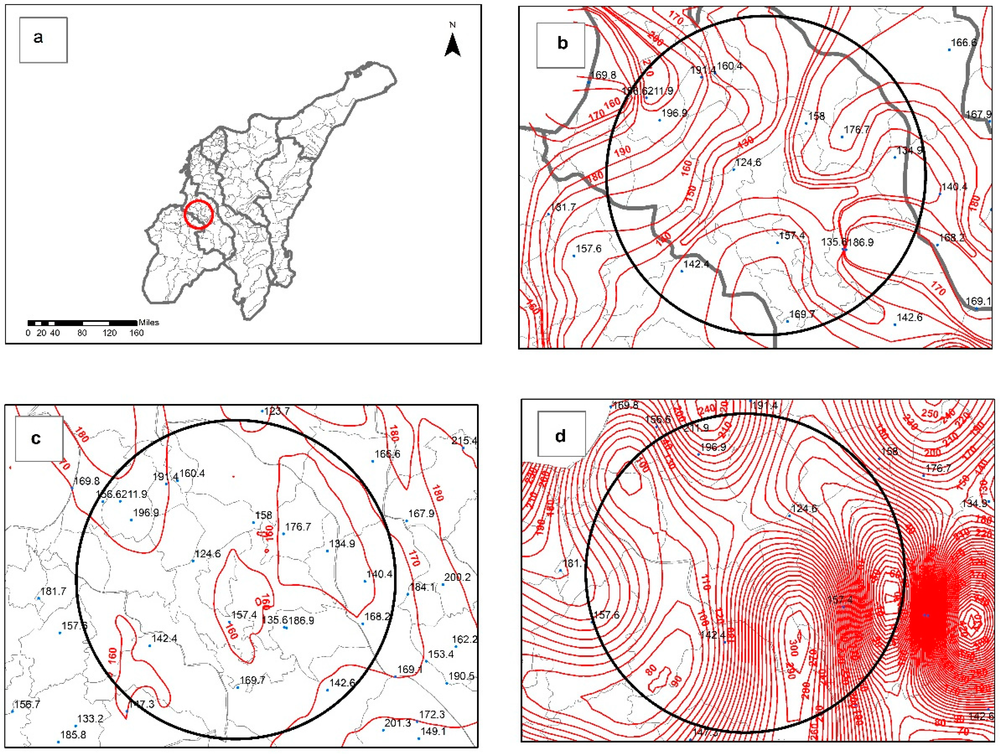
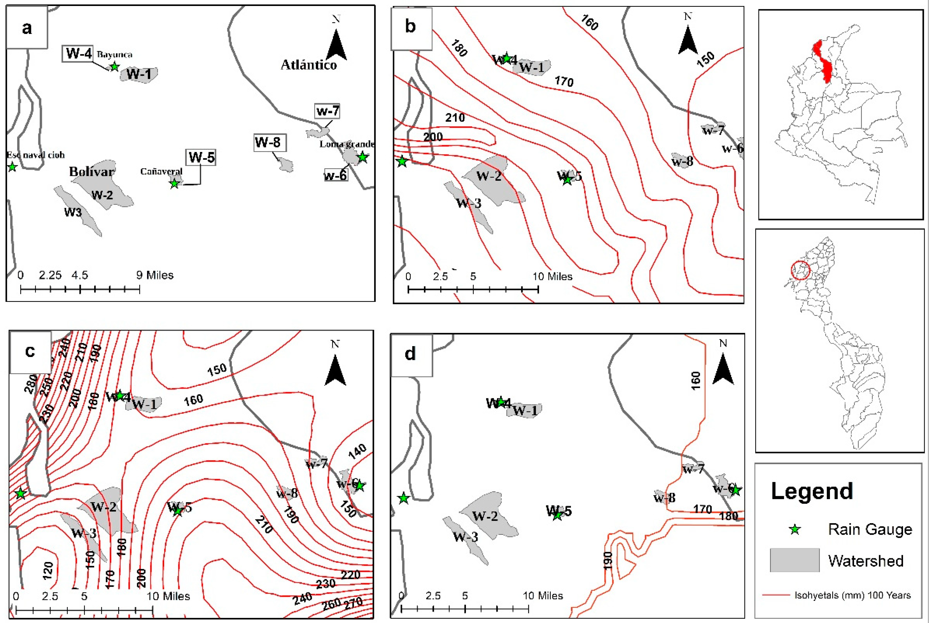
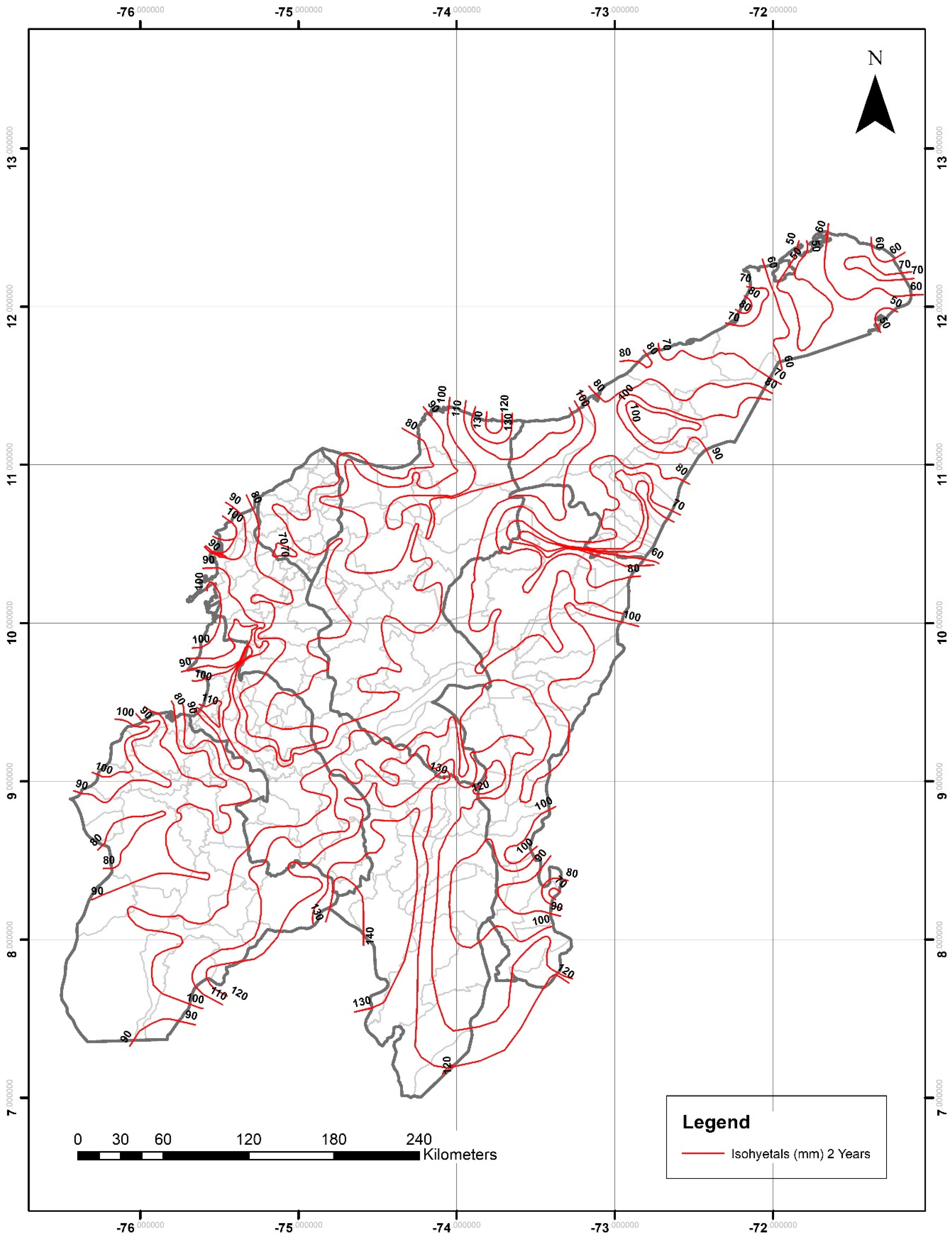
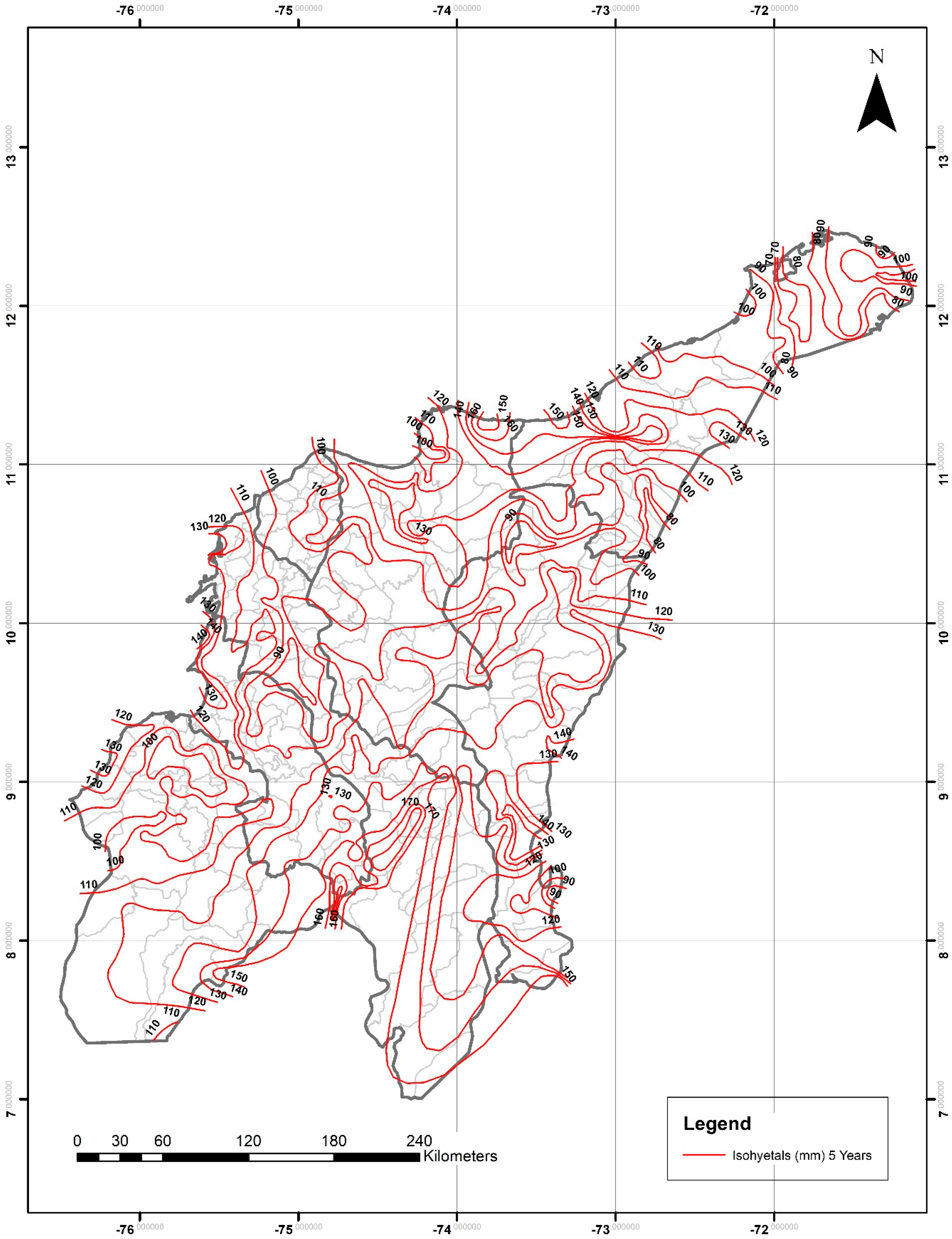
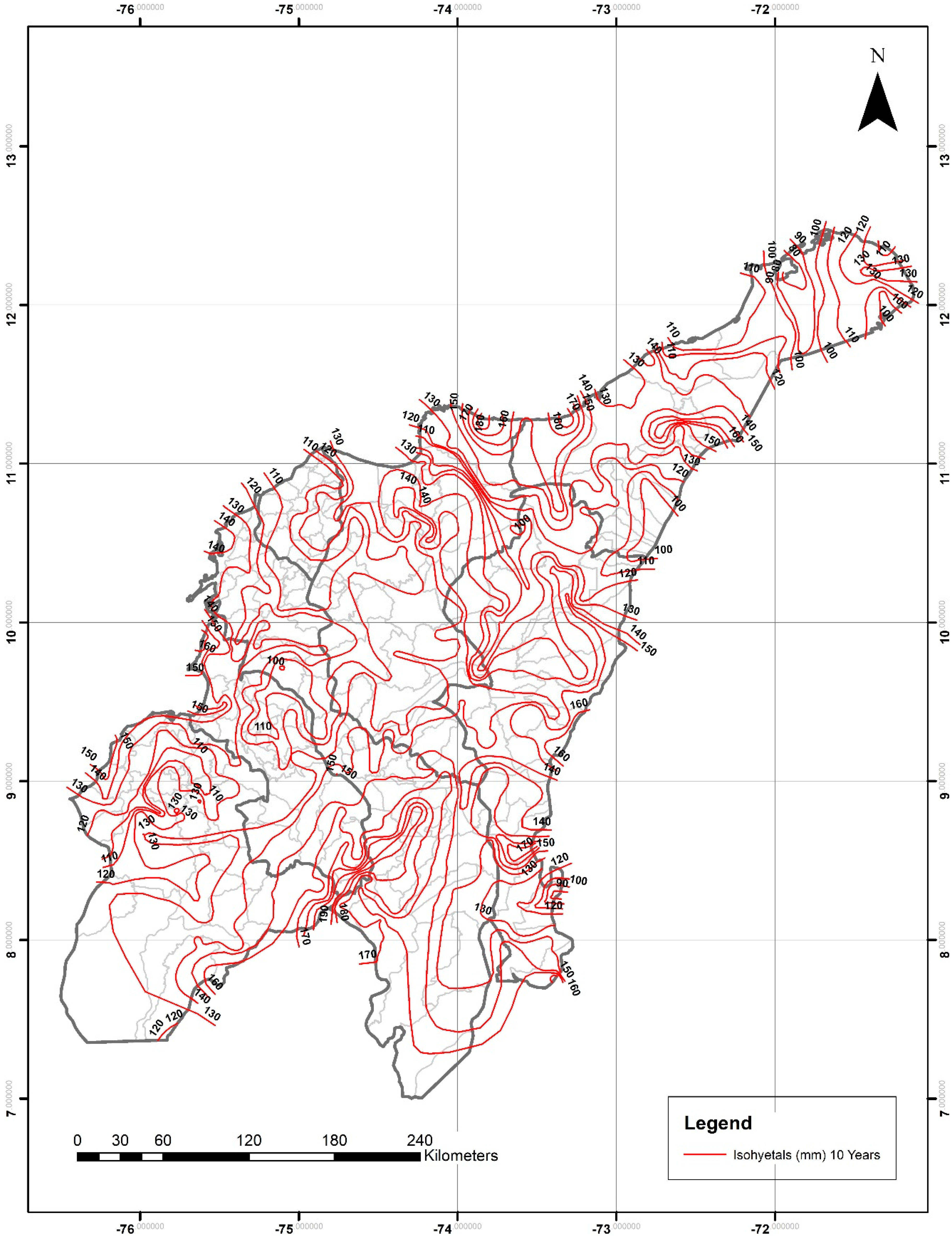
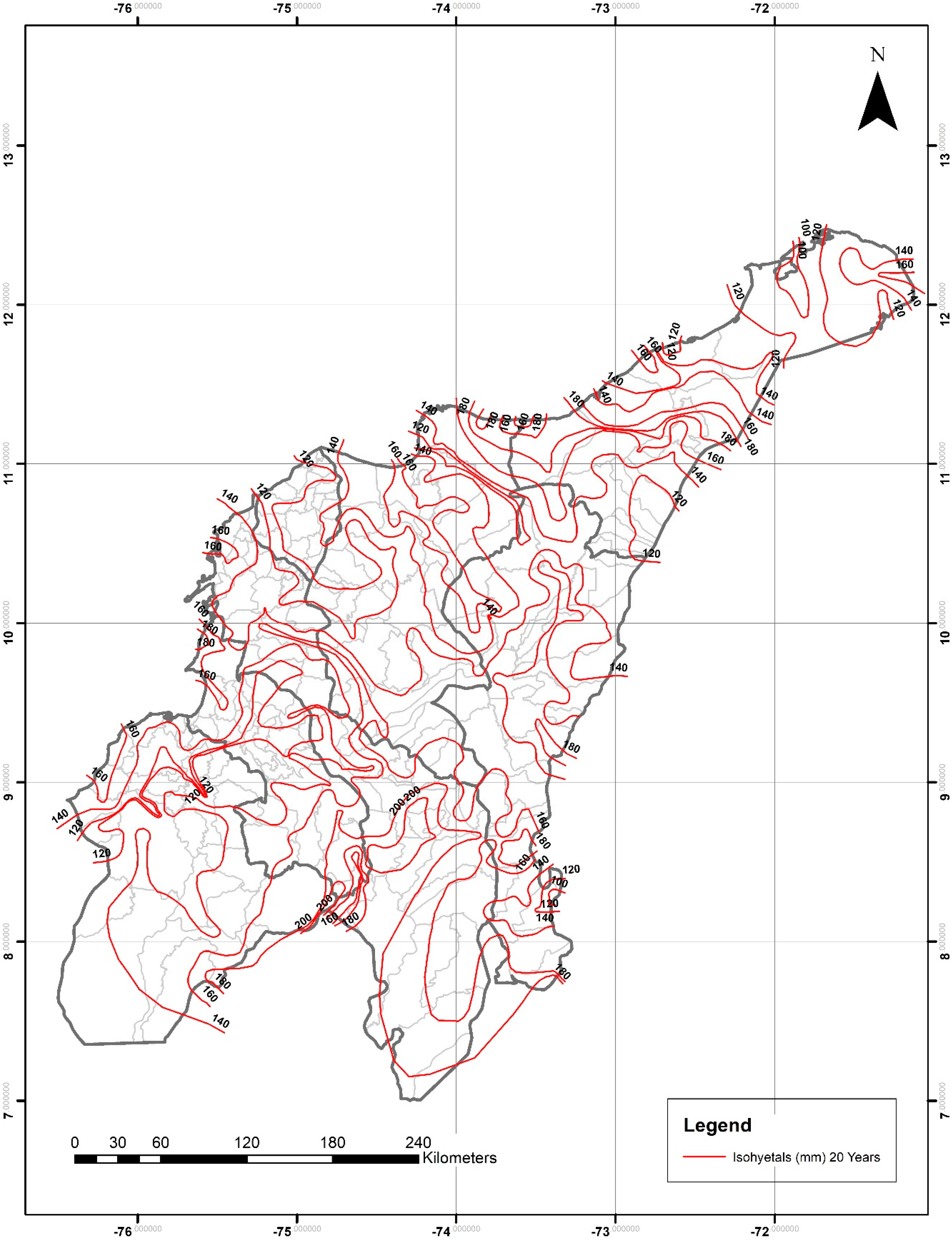
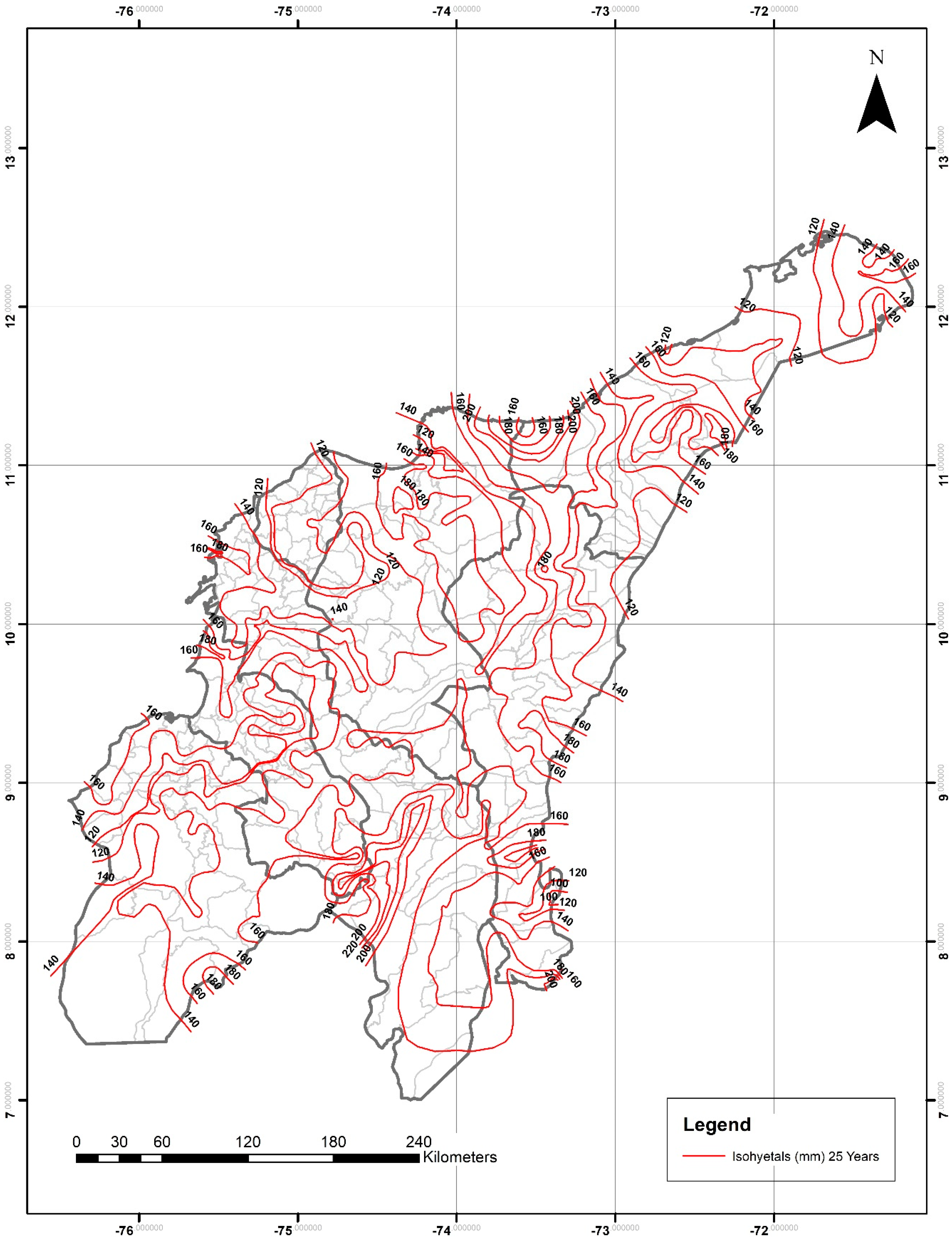
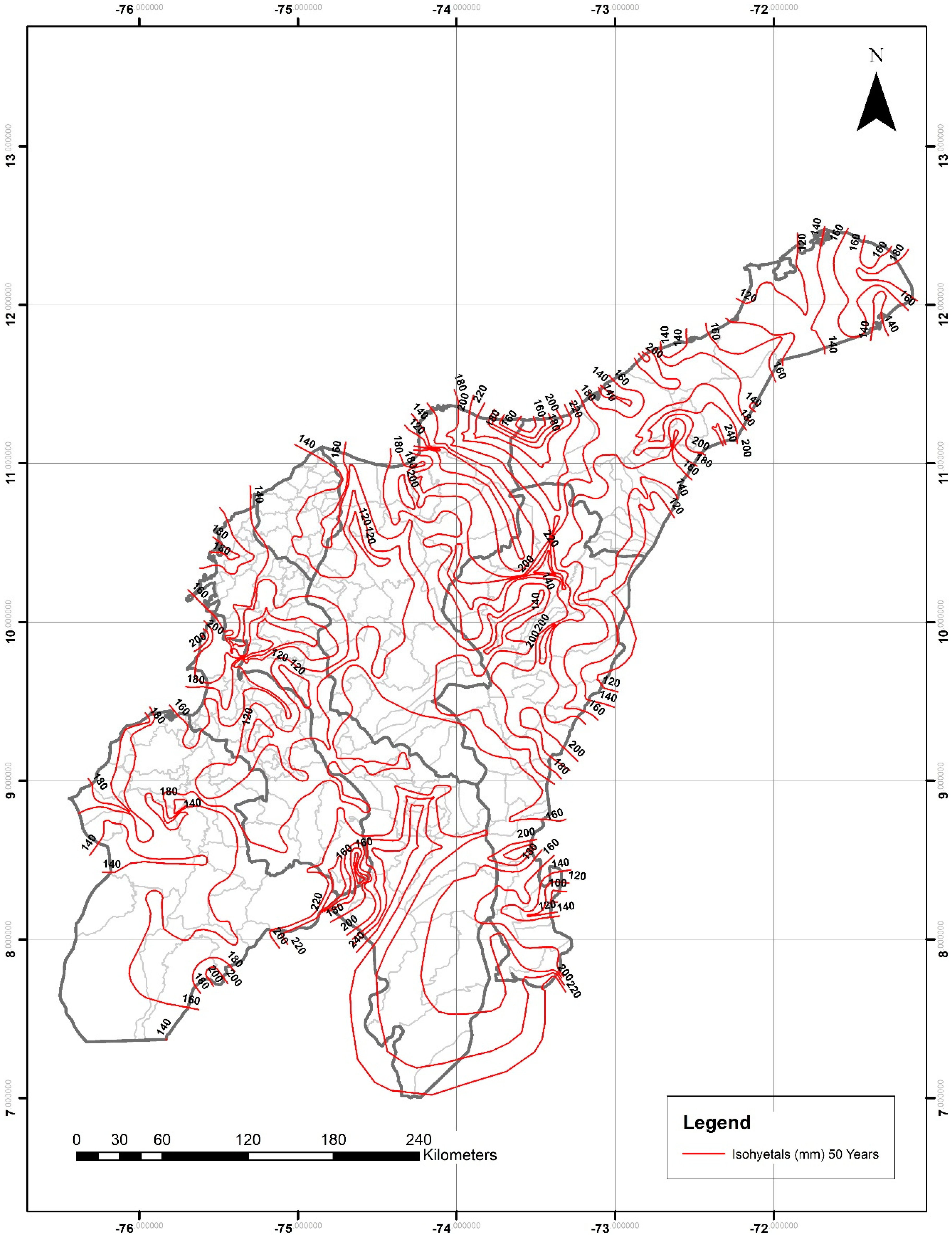
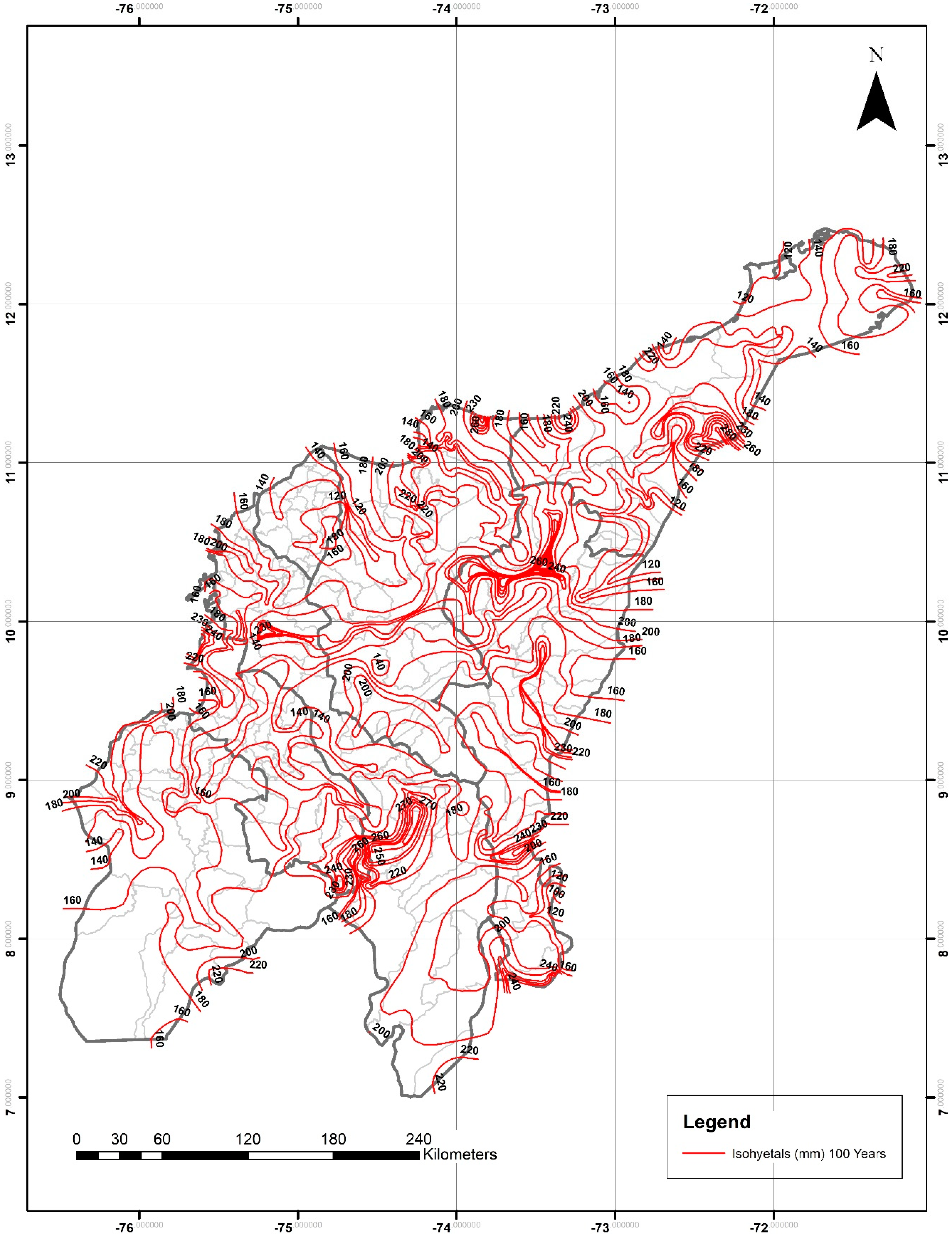
3.4. Drawing of Isohyetals for Different Return Periods

A spreadsheet with the geographical location (latitude and longitude) of the 318 rain gauges along with their corresponding estimated P_24h-max values for the different return periods was exported into ArcGIS (Version 10.4.1, ESRI Inc., Redlands, CA, USA) to create a layer for further processing. Given the large density of rain gauges in some areas, three interpolation methods were used to generate the isohyetals: Inverse Distance Weighting (IDW), Ordinary Kriging (OK), and Spline (SP), in order to evaluate their performance prior to selecting one of the methods [61,62,63]. Default ArcGIS inputs were used in all methods since a sensitivity analysis done for each of the methods by changing the various inputs showed no major changes or improvements in the areas with noticeable alignment discrepancies. The ArcGIS inputs for the three methods are shown in

Table 3. ArcGIS Inputs for each interpolation method.

Interpolation Method	Z-Value	Cell Size	Search Radius
Spline (Regularized)	2	0.021	Variable. Number of points: 12. Weight: 0.1.
Ordinary Kriging	2	0.021	Variable. Number of points: 12
IDW	2	0.021	Variable. Number of points: 12.

.

3.5. Assessing the Interpolation Methods

The accuracy of each interpolation method in predicting a P_24h-max value for a given return period was evaluated by means of the Root Mean Squared Error (RMSE) (Equation (10)), the Relative Error (REr) (Equation (11)), the Bias or Mean Deviation (MDv) (Equation (12)), and the Nash–Sutcliffe Coefficient (NSC) (Equation (13)). In Equations (10)–(13), P_sim is the simulated areal precipitation from each of the Interpolation Methods (P_24h-max-IM), $\overline{P_{sim}}$ is the average simulated areal precipitation, and P_true is P_24h-max-RG, which has been considered the true value due to the proximity to the rain gauges. RMSE and REr measure the accuracy, whereas MDv tests the bias. The lower the values of RMSE, REr, and MDv, the better the interpolation method. The NSC, in particular, is widely used in hydrology to assess the prediction power of a model, and it ranges from −∞–one, where negative values indicates that it is better to use the mean of the measured data (true value) than the predicted/simulated value; a value of zero (or close to zero) indicates that either the mean of the measured values or the predicted/simulated value can be used indistinctively; and a value equal to one indicates good agreement between the predicted/simulated and the measured data (true value) [9,64,65].

$$\mathrm{RMSE}=\sqrt{\frac{{{\displaystyle \sum }}_{i=1}^n{\left[P_{sim}-P_{true}\right]}^2}{n}}$$

(10)

$$\mathrm{REr}(\%)=\left|\frac{P_{true}-P_{sim}}{P_{true}}\right|\times 100$$

(11)

$$\mathrm{MDv}\left(\mathrm{Bias}\right)=\frac{{{\displaystyle \sum }}_{i=1}^n\left(P_{true}-\overline{P_{sim}}\right)}{n}$$

(12)

$$\mathrm{NSC}=1-\frac{{{\displaystyle \sum }}_{i=1}^n{\left(P_{true}-P_{sim}\right)}^2}{{{\displaystyle \sum }}_{i=1}^n{\left(P_{true}-\overline{P_{sim}}\right)}^2}$$

(13)

4. Results and Discussion

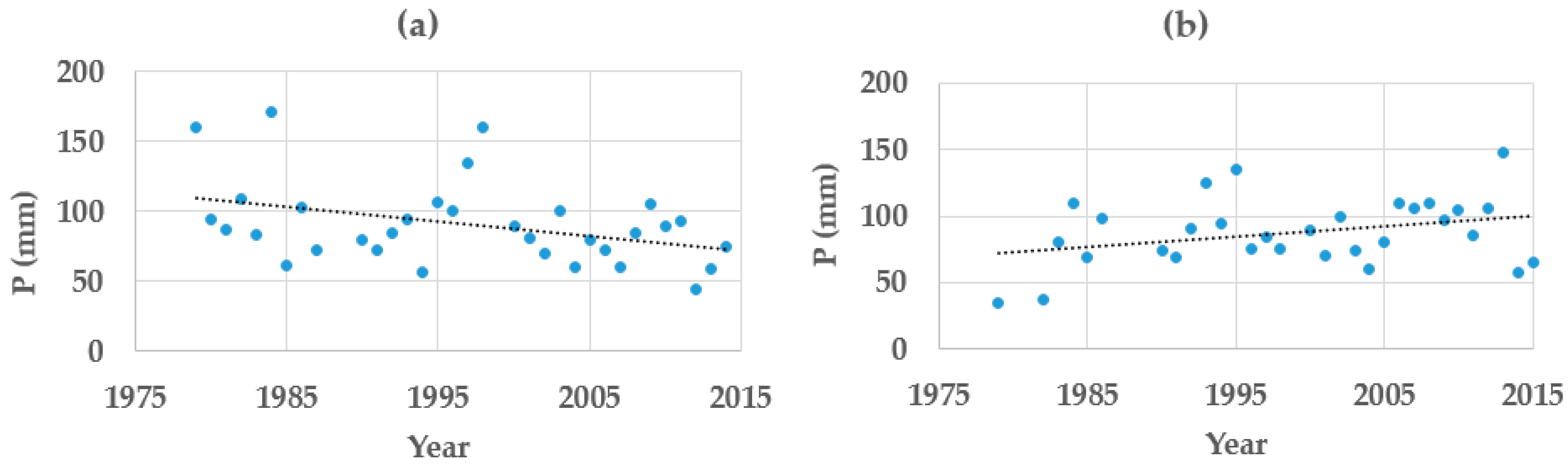
4.1. Multiannual Time Series of P_24h-max Values

Scatter plots of the multiannual series of P_24h-max of each rain gauge revealed that there might be regionalization of the daily maximum rainfall trends within the departments that need to be further explored and analyzed, as it was observed that rainfall observations showed a noticeable increasing or decreasing trend line over time, which may indicate (a) a change in the rainfall pattern due to, among others, anthropogenic factors and (b) that a non-stationary frequency analysis is more suitable for the rainfall data of those rain gauges at a local level [66,67]. Figure 3 shows the scatter plot and the trend lines of the rain gauges Puerto Giraldo and Los Campanos located in the department of Atlántico.

4.2. CDFs and Frequency Analysis

As previously mentioned, in Colombia, it is a common practice among hydrologist to use the Gumbel distribution solely for rainfall frequency analysis. However, results presented in

Table 4. Best CDFs per department. GEV, Generalized Extreme Value; LP3, Log-Pearson 3.

Department	Best-Fit CDF			Total
	GEV	Gumbel	LP3
Guajira	21	18	5	44
Cesar	27	21	12	60
Magdalena	26	15	14	55
Atlántico	7	6	0	13
Bolívar	23	22	12	57
Sucre	16	14	2	32
Córdoba	26	12	14	52
Antioquia	3	0	0	3
Santander	1	0	0	1
Norte de Santander	0	1	0	1
Total	150	109	59	318

show that GEV is the CDF that best fit the majority of the rain gauges analyzed in this study with 47.2%, followed by Gumbel with 34.3% and LP3 with 18.5%.

Furthermore, based on the value obtained for the shape parameter (k), the 150 rain gauges where GEV was found to be the best fit were further analyzed to determine whether the GEV corresponded to a Type 2 (Fréchet) or Type 3 (Weibull) Extreme Value (EV) distribution.

Table 5. EV distribution equivalence.

Department	EV Type Equivalence of the GEV		Total
	EV-3 (Weibull) (k > 0)	EV-2 (Fréchet) (k < 0)
Guajira	12	9	21
Cesar	17	10	27
Magdalena	19	7	26
Atlántico	6	1	7
Bolívar	19	4	23
Sucre	10	6	16
Córdoba	16	10	26
Antioquia	1	2	3
Santander	0	1	1
Norte de Santander	N/A	N/A	0
Total	100	50	150

summarizes the EV Type 2 and 3 totals for each department.

Taking for granted that all rainfall time series fit the Gumbel distribution could lead to either under- or over-estimation of the design rainfall. This is clearly shown in

Table 6. P_24-max values for different return periods.

Rain Gauge Name (Department)	P24h-max (mm)							CDF	Chi-Squared (X2)
	Return Period (Year)
	2	5	10	20	25	50	100
Santa Ana (Bolívar)	101.1	124.7	135.9	144.3	146.6	152.5	157.2	GEV	2.15
	96.0	126.9	147.3	166.9	173.1	192.3	211.3	Gumbel	6.52
	99.2	124.7	138.2	149.1	152.2	161.0	168.5	LP3	3.12
Palo Alto (Magdalena)	95.4	126.8	149.0	171.5	178.8	202.2	226.7	GEV	2.91
	96.5	127.3	147.7	167.2	173.4	192.5	211.5	Gumbel	6.04
	96.1	127.5	148.9	169.9	176.6	197.7	219.3	LP3	4.48

, where, according to the chi-squared test, the Gumbel distribution was not the best fit in any of the cases. The situation became more critical at higher return periods such as 50 years and 100 years (two of the most-used return periods in hydrological analysis for stormwater management and in consideration for flood studies). For the 100-year return period, the differences observed between GEV and Gumbel distributions at rain gauges Santa Ana and Palo Alto were 54.1 mm and 15.2 mm, respectively. Not selecting the most appropriate distribution can negatively impact, for instance, the design of hydraulic structures for stormwater management and/or the delineation of flood-prone areas.

In general, the GEV and Gumbel distributions were demonstrated to be the most suitable for rainfall frequency analysis in the Caribbean region of Colombia. The LP3 distribution showed both poor performance (in some cases, the datasets did not even fit) in most of the rain gauges analyzed and a tendency to underestimate when compared to the values obtained by either GEV or Gumbel distributions, irrespective of being (or not) the best fit of the three.

4.3. Interpolation Methods Assessment

After visually inspecting the isohyetal alignments, it was observed that the IDW method had less inconsistencies, among all. Nonetheless, in some areas, it was necessary to adjust manually the isohyetals’ alignment generated by the IDW method (the manually-adjusted IDW method will be referred to as IDW adjusted). Figure 4 depicts the differences among the interpolation methods. Isohyetals by the OK method (Figure 4c) evidenced: (a) the presence of small oval-shaped isohyetals with the same rainfall value of the larger oval they were within and (b) large areas between neighboring rain gauges with no isohyetals (“dead or no-variation zones”), which could affect the estimation of the areal precipitation for a given watershed (the problem was most evident as the return period decreased). The spline method (Figure 4d) generated, in some cases, isohyetals with negative values. Isohyetals drawn by the IDW method (Figure 4b), despite the fact that a few minor adjustments were manually made in some areas, did not show the setbacks of the other two methods. The IDW method, in spite of its simplicity compared to other interpolation methods like the OK method, is recommended when the data are irregularly distributed like the rain gauges used in this study [68,69].

In addition to the visual inspection, the accuracy of all generated maps (by each of the interpolation methods) to estimate P_24h-max values for a given return period was evaluated in eight watersheds with various area sizes and located at different distances from neighboring rain gauges. Five watersheds are located in the northern part of the department of Bolívar. Watersheds 1, 2, and 3 (W-1, W-2, and W-3) are close to the rain gauges Bayunca, Cañaveral, and Escuela Naval-CIOH, respectively. The rain gauges Bayunca and Cañaveral are located within Watersheds 4 and 5 (W-4 and W-5). Furthermore, three watersheds (W-6, W-7, and W-8) located in the vicinity of the rain gauge Loma Grande (department of Atlántico) were selected to validate the performance of the isohyetal methods in areas with nearby rain gauges not included in this study (Loma Grande had less than thirty years of observations).

Table 7. Watersheds’ (W) information.

Watershed	Area (ha)	Distance to Nearest Rain Gauge in km
W-1	651.7	3.3 (Bayunca)
W-2	2146.5	9.2 (Cañaveral)
W-3	710.7	11.2 (Escuela Naval-CIOH)
W-4	52.4	0.0 (rain gauge Bayunca is within the watershed)
W-5	154.0	0.0 (rain gauge Cañaveral is within the watershed)
W-6	460.4	0.0 (rain gauge Loma Grande is within the watershed)
W-7	200.6	6.0 (Loma Grande)
W-8	204.6	9.2 (Loma Grande)

summarizes the watersheds’ area and distance from the centroid to the nearest rain gauge. Figure 5 depicts the location and the isohyetals at each of the watersheds for a 100-year return period.

Watersheds areal P_24h-max for return periods of 2, 5, 10, 20, 25, 50, and 100 years were estimated from each of the isohyetal maps (P_24h-max-IM) and compared to the resulting P_24h-max values calculated via frequency analysis of the time series of each of the nearby rain gauges (P_24h-max-RG).

The estimated values of P_24h-max-RG and P_24h-max-IM are presented in

Table 8. Values of P_24h-max-RG and areal P_24h-max-Interpolation Method (IM).

Rain Gauge		P24h-max-RG (mm)
		Tr (Years)
		2	5	10	20	25	50	100
Bayunca		100.5	127.6	140.6	150.5	153.5	160.5	166.3
Cañaveral		86.6	115.7	136.4	157.2	164.1	185.8	208.5
Escuela Naval-CIOH		87.5	116.7	133.7	148.6	153.0	165.9	177.6
Loma Grande		75.4	101.3	118.4	134.8	140.0	156.1	172.0
Interpolation Method	Watershed	Areal P24h-max-IM (mm)
IDW Adjusted	W-1	95.0	125.0	135.0	146.2	155.0	155.4	165.0
	W-2	89.9	115.0	135.0	162.4	169.0	181.4	187.1
	W-3	85.0	115.0	135.0	155.5	156.5	170.7	180.1
	W-4	96.7	125.0	138.8	154.0	155.0	163.7	165.0
	W-5	85.0	115.0	135.0	155.0	165.0	175.0	205.0
	W-6	70.0	100.0	110.0	120.0	122.2	136.9	155.0
	W-7	75.0	100.0	110.0	124.9	129.0	145.0	155.0
	W-8	75.0	100.0	114.2	135.0	137.1	149.1	155.0
Spline	W-1	91.8	116.7	128.8	138.7	141.4	149.8	157.1
	W-2	76.5	100.7	115.1	129.9	133.9	149.7	161.6
	W-3	75.0	91.9	104.4	115.2	117.0	129.3	140.9
	W-4	103.8	127.1	144.0	154.1	155.0	164.3	167.7
	W-5	80.0	115.0	139.0	155.0	165.0	185.0	206.8
	W-6	70.0	95.0	110.0	120.0	123.2	133.1	178.1
	W-7	70.0	95.0	110.0	125.0	125.0	142.3	156.5
	W-8	75.0	100.0	115.0	135.0	142.4	158.8	142.4
Ordinary Kriging	W-1	95.0	125.0	125.0	136.3	145.0	155.0	165.0
	W-2	86.0	116.9	125.4	145.0	145.0	155.0	165.0
	W-3	95.0	119.3	127.0	145.0	145.0	155.0	165.0
	W-4	95.0	125.0	125.0	145.0	145.0	155.0	165.0
	W-5	85.0	115.0	125.0	135.0	145.0	155.0	165.0
	W-6	80.0	100.0	120.0	130.0	140.0	150.0	160.0
	W-7	80.0	100.0	120.0	131.4	140.0	150.0	160.0
	W-8	80.5	100.0	121.2	135.0	140.0	153.1	164.0

. P_24h-max-RG is the value obtained via frequency analysis of the precipitation data for all return periods at each of the rain gauges used for validation. P_24h-max-IM is the estimated areal precipitation of each watershed by means of the isohyetal method. The observed two-year P_24h-max-RG values ranged from 75.4 mm (Loma Grande) to 100.5 mm (Bayunca). Among all rain gauges, Loma Grande had the lowest P_24h-max-RG for almost all return periods, except for 100 years. The highest P_24h-max-RG values calculated were for the rain gauges of Bayunca (for 2 years, 5 years, and 10 years) and Cañaveral (for 20 years, 25 years, 50 years, and 100 years). The minimum two-year P_24h-max-IM values estimated were 91.8 mm (spline), 76.5 mm (spline), 75.0 mm (spline), 95.0 mm (OK), 80.0 mm (OK and spline), 70.0 mm (spline and IDW adjusted), 70.0 mm (spline), and 75.0 mm (IDW adjusted and spline) for W-1, W-2, W-3, W-4, W-5, W-6, W-7, and W-8, respectively. With the IDW adjusted method, the maximum values for the 100-year P_24h-max-IM were 165.0 mm, 187.1 mm, 180.1 mm, and 165 mm for W-1, W-2, W-3, and W-4, respectively. With the spline method, the maximum values computed for 100 years were 206.0 mm for W-5 and 178.1 mm for W-6. With the OK method, the maximum values of P_24h-max-IM for 100 years were 160.0 mm and 164.0 mm for W-7 and W-8, respectively.

With the values estimated in Table 8, the performance of the interpolation methods at each of the watershed was tested via REr, and the overall performance of each interpolation method in predicting P_24h-max for a given return period in all watersheds (n = 8) was tested via RMSE, MDv, and NSC (

Table 9. Interpolation method performance at each watershed.

Int. Method	Watershed	Relative Error
		Tr (Years)
		2	5	10	20	25	50	100
IDW Adjusted	W-1	5.8%	2.1%	4.2%	3.0%	1.0%	3.3%	0.8%
	W-2	3.7%	0.6%	1.0%	3.2%	2.9%	2.4%	11.4%
	W-3	3.0%	1.5%	1.0%	4.5%	2.3%	2.8%	1.4%
	W-4	4.0%	2.1%	1.3%	2.3%	1.0%	1.9%	0.8%
	W-5	1.8%	0.6%	1.0%	1.4%	0.5%	6.2%	1.7%
	W-6	7.8%	1.3%	7.6%	12.3%	14.6%	14.0%	11.0%
	W-7	0.6%	1.3%	7.6%	7.9%	8.5%	7.7%	11.0%
	W-8	0.6%	1.3%	3.7%	0.1%	2.1%	4.7%	11.0%
Spline	W-1	9.5%	9.4%	9.2%	8.5%	8.6%	7.1%	5.8%
	W-2	13.2%	14.9%	18.5%	21.0%	22.6%	24.1%	29.0%
	W-3	16.7%	17.0%	28.1%	29.0%	30.7%	28.3%	26.1%
	W-4	3.2%	0.4%	2.3%	2.3%	1.0%	2.3%	0.8%
	W-5	8.2%	0.6%	1.9%	1.4%	0.5%	0.4%	0.8%
	W-6	7.8%	6.6%	7.6%	12.3%	13.6%	17.3%	3.4%
	W-7	7.8%	6.6%	7.6%	7.8%	12.0%	9.7%	9.9%
	W-8	0.6%	1.3%	3.0%	0.1%	1.7%	1.7%	20.8%
Ordinary Kriging	W-1	5.8%	2.1%	12.5%	10.5%	5.9%	3.6%	0.8%
	W-2	0.6%	1.0%	8.7%	8.4%	13.2%	19.9%	26.4%
	W-3	7.9%	2.2%	5.2%	2.5%	5.5%	7.0%	7.6%
	W-4	5.8%	2.1%	12.5%	3.8%	5.9%	3.5%	0.8%
	W-5	1.8%	0.6%	9.1%	16.4%	13.2%	19.9%	26.4%
	W-6	5.7%	1.3%	1.3%	3.7%	0.0%	4.1%	7.5%
	W-7	5.7%	1.3%	1.3%	2.6%	0.0%	4.1%	7.5%
	W-8	6.2%	1.3%	2.3%	0.1%	0.0%	2.0%	4.9%
		Root Mean Squared Error (RMSE)
IDW Adjusted	All Watersheds	0.37	0.15	0.45	0.62	0.66	0.76	0.96
Spline		0.80	1.06	1.23	1.40	1.53	1.60	1.78
Ord. Kriging		0.52	0.17	0.85	0.86	0.85	1.22	1.62
		Mean Deviation (Bias)
IDW Adjusted	All Watersheds	2.05	1.53	3.74	1.93	2.43	6.21	9.50
Spline		5.74	8.23	9.59	11.95	13.16	14.32	16.52
Ord. Kriging		−1.07	0.75	6.79	8.21	7.90	12.34	16.78
		Nash–Sutcliffe Coefficient (NSC)
IDW Adjusted	All Watersheds	0.88	0.97	0.76	0.39	0.37	0.49	0.54
Spline		0.56	0.26	−0.11	−0.29	−0.36	−0.26	−0.09
Ord. Kriging		0.76	0.97	0.27	0.24	0.23	0.08	0.03

Gray cells indicate that a method different from IDW adjusted performed best. Green cells indicate a Relative Error (REr) value above five percent.

).

The REr values in Table 9 show how the IDW adjusted outperformed the other two methods in almost all watersheds except in 18 cases (gray cells) out of 168 (nine of those 18 cases occurred in watersheds where the rain gauge was within them). With respect to the watersheds having a rain gauge within them (W-4, W-5, and W-6), better REr results were obtained in the IDW adjusted method, except for W-6, where the OK method predicted values closer to the ones calculated via frequency analysis. The IDW adjusted method showed REr estimates ranging from 0.8–4% for W-4, 0.6–6.2% for W-5, and 1.3–14.6% for W-6. The spline method had REr estimates that oscillated from 0.4–3.2% for W-4, 0.4–8.2% for W-5, and 3.4–17.3%. The REr values obtained through the OK method ranged from 0.8–12.5% for W-4, from 0.6–26.4% for W-5, and from 0.0–7.5% for W-6. The IDW adjusted method reported fifteen REr values above 5%, of which only two cases were greater than 10% (the highest was 14.6%). The spline method reported 36 cases where REr values were above 5%, with 17 values above 10% (the highest was 20.8%). Finally, the OK method had 27 cases where REr estimates were above 5%, with 11 values above 10% (the highest was 26.4%). When the performance of the interpolation methods was evaluated based on the distance between the watershed and the rain gauge, once again, the IDW adjusted method exhibited better results, with a few exceptions observed (gray cells in W-2, W-7, and W-8). For W-1 and W-3 (respectively, the closest and the furthest), lower REr values were obtained with the IDW adjusted method. For W-2, located at 9.2 km of its corresponding closest rain gauge, the IDW adjusted method had lower estimates of REr for all return periods, except at two years, where the OK method was best. However, the IDW adjusted method reported an error of only 3.7%. For W-8, also located at 9.2 km, for return periods of 10 years, 25 years, and 50 years, the OK and spline methods were best. Nonetheless, all REr values observed for the IDW adjusted method were lower than 5%, except for the return period of 100 years with a value of 11%. For W-7, located at 6.0 km from the rain gauge Loma Grande, the OK method reported lower REr values, which ranged from 0.0–7.5%. The IDW adjusted and spline methods reported similar REr values (less than 5%) in most of the return periods, except for the return period of 100 years, where values of 11% and 20.8% were obtained for the IDW adjusted and spline methods, respectively. As for the return periods of 50 years and 100 years, two of the most-used return periods when evaluating the performance of hydraulic structures (e.g., culverts, bridges, and open channels) and in flood mitigation and stream restoration projects, the IDW adjusted method reported better results, with only six cases (four for the spline method and two for the OK method) out of 42, where the other two methods outperformed. The IDW adjusted method reported four cases above 10% (the highest was 14%), while spline had six cases (the highest was 20.8%). Although the OK method also reported four cases with REr values greater than 10%, the maximum value was 26.4%, which is the largest of the three methods. Irrespective of the watershed size and/or distance from a nearby rain gauge, these results are not only indicative that the IDW adjusted method performed best in the majority of the watersheds where the rain gauge was within them (W-4, W-5, and W-6), but also—and most importantly—in areas distant from a rain gauge where the design rainfall estimation was most needed, since in watersheds where a rain gauge is within them, it is always recommended to calculate the design rainfall directly from the rainfall observations.

As for the overall performance of the interpolation methods, the IDW adjusted method had the best results (RMSE, MDv, and NSC) in the majority of the cases. The OK method showed lower bias (MDv) values for two occasions (−1.07 mm and 0.75 mm for return periods of two and five years; negative values indicate that average simulated value was higher than the true value). This notwithstanding, the IDW adjusted method estimates were low as well (2.05 mm and 1.53 mm for return periods of two and five years). A closer look at the isohyetal alignment of both methods within the assessed area revealed that the OK method alignment for isohyetals of 70 mm, 80 mm, 90 mm, and 100 mm did not pass through several rain gauges they were supposed to have (dead or no-variation zones). This would have resulted in high error values for the OK method had other watersheds been selected. In general, the results indicate that the values from the IDW adjusted method showed less bias (2.5 mm–9.5 mm) than the other two methods (5.74–16.52 mm and −1.07–16.78 mm for the spline and OK methods, respectively), where the bias was more noticeable as the return period increased. This can lead to serious implications, especially at return periods of 50 years and 100 years, which are two of the most used in the design of hydraulic structures for both stormwater management and flood mitigation projects. As for the prediction power, the IDW adjusted method outperformed the other two methods with NSC values greater than or equal to 0.39, indicating good agreement between the true and simulated variables. For the spline method, the NSC was above zero only in return periods of two and five years. The remaining return periods showed negative values, implying that the average value was a better predictor. Similar results were observed for the OK method, with values closer to zero as the return period increased, which signifies that either the average or the true values were better predictors. The NSC values for the spline and OK methods are consistent with the bias results: poor performance in predicting P_24h-max when compared with the IDW adjusted method.

In sum, the results above confirm that the performance of an interpolation method should always be assessed prior to its selection [68,69,70,71,72,73,74,75]. This is of great importance, especially, because the OK method has become one of the most widely-preferred interpolation methods to the point that some do not even question its adequacy due to it typically showing good results.

4.4. Isohyetal Maps for Different Return Periods

The seven isohyetals maps of daily maximum precipitation for return periods of 2, 5, 10, 20, 25, 50, and 100 years drawn by means of the IDW adjusted method for the Colombian Caribbean region are shown in Figure 6, Figure 7, Figure 8, Figure 9, Figure 10, Figure 11 and Figure 12. The statistical analysis results demonstrated that areal P_24h-max can be estimated by means of the isohyetal maps proposed in this study. However, the final decision of using the maps shall be at the user’s discretion based on his/her experience and knowledge of the area where the areal P_24h-max is intended to be estimated. It is then recommended that a frequency analysis of the multiannual series be performed, and the results shall be compared to those estimated through the isohyetal maps in order to rule out any major discrepancies that could potentially affect the calculation of the design streamflow value and subsequent sizing of hydraulic structures.

For the department of Guajira, P_24h-max isohyetals ranged from 50–120 mm for two years, 70–150 mm for 5 years, 90–160 mm for 10 years, from 100–180 mm for 20 years, 120–200 mm for 25 years, from 120–240 mm for 50 years, and from 120–280 mm for 100 years. The lowest and highest values were observed in the northeastern and northwestern areas, respectively.

For the department of Magdalena, P_24h-max isohyetals ranged from 80–130 mm for two years, 90–160 mm for five years, 110–170 mm for 10 years, from 120–180 mm for 20 years, 120–200 mm for 25 years, from 120–240 mm for 50 years, and from 120–260 mm for 100 years. The lowest and highest values were observed in the eastern and northern areas, respectively.

For the department of Cesar, P_24h-max isohyetals ranged from 80–120 mm for two years, 90–150 mm for five years, 100–170 mm for 10 years, from 120–180 mm for 20 years, 120–200 mm for 25 years, from 120–220 mm for 50 years, and from 120–260 mm for 100 years. The lowest and highest values were observed in the northeastern and southern areas, respectively.

For the department of Atlántico, P_24h-max isohyetals ranged from 70–90 mm for two years, 100–110 mm for five years, 100–120 mm for 10 years, from 120–140 mm for 20 years, 120–140 mm for 25 years, from 140–160 mm for 50 years, and from 120–180 mm for 100 years. The lowest and highest values were observed in the central-eastern and southern areas, respectively. This was the department with the smallest ranges of P_24h-max values mainly due to its total area (3385.1 km²) and topography.

For the department of Bolívar, P_24h-max isohyetals ranged from 90–140 mm for two years, 90–170 mm for five years, 100–190 mm for 10 years, from 120–200 mm for 20 years, 120–200 mm for 25 years, from 120–240 mm for 50 years, and from 140–270 mm for 100 years. The lowest and highest values were observed in the northern and southwestern areas, respectively.

For the department of Sucre, P_24h-max isohyetals ranged from 90–130 mm for two years, 90–160 mm for five years, 100–190 mm for 10 years, from 120–200 mm for 20 years, 120–200 mm for 25 years, from 120–240 mm for 50 years, and from 140–250 mm for 100 years. The lowest and highest values were observed in the northeastern and southeastern areas, respectively.

For the department of Córdoba, P_24h-max isohyetals ranged from 80–130 mm for two years, 100–160 mm for five years, 110–190 mm for 10 years, from 120–200 mm for 20 years, 120–200 mm for 25 years, from 120–220 mm for 50 years, and from 140–240 mm for 100 years. The lowest and highest values were observed in the northwestern and southeastern areas, respectively.

5. Conclusions

Unlike other countries, Colombia, currently, does not have any official document that compiles a series of recommended methodologies for frequency analysis for a particular region. In this context and contrary to what is the common practice, the Gumbel distribution was not the best fit for most of the time series analyzed. Instead, and according to the chi-squared test, the GEV distribution was shown to be the best fit among the three CDFs used in majority of the datasets. Only 34.3% of the rain gauges fit the Gumbel distribution, while 47.2% of them fit the GEV distribution. LP3, on the other hand, did not work well among the rain gauges analyzed. Based on the results of this study, GEV and Gumbel are the most recommended distributions for the Caribbean region of Colombia.

With respect to the best interpolation method for generating isohyetals in the study area, the IDW method outperformed both the spline and the ordinary kriging methods. These results demonstrate that geostatistically-based interpolation methods (e.g., ordinary kriging) are not always the best selection as many typically take for granted.

According to the results of the REr, RMSE, MDv, and NSC, the areal P_24h-max estimated with the resulting isohyetal maps (by the IDW adjusted method) of this study were close to the true value and can be used to select a design rainfall for a given return period. This is of particular significance given the large amount of ungauged areas within the Colombian Caribbean region where many hydrological studies (made by either international or local consulting companies) are based on the utilization of neighboring rain gauges that sometimes are located at remote distances that do not guarantee the reliability and/or accuracy of the derived design rainfall. The isohyetal maps generated in this study are the first step in developing similar ones for the remaining four regions of Colombia. The 318 multiannual P_24h-max time series analyzed were assumed to be stationary. However, increasing and decreasing trends were observed in some of the time series, suggesting the presence of non-stationarity, which, if confirmed, could result in higher or lower values of point P_24h-max (at the rain gauge). The possible modifications of the isohyetal alignments in certain areas may or may not alter the total areal P_24h-max of a given watershed, since, unlike point rainfall, the areal rainfall is calculated differently. It depends on both the isohyetal alignment (which, in this case, will vary based on the stationary versus the non-stationary P_24h-max value obtained) and the watershed size and distance from the nearest rain gauges, which define how much area of the watershed is covered by each isohyetal (the weighted area). In other words, a change in the value of point rainfall does not necessarily imply a major change in the areal rainfall. Because of that, the authors’ future work will address: (a) P_24h-max regionalization at each of the seven departments of the Colombian Caribbean region, (b) the monotonic trend of the multiannual P_24h-max time series via Mann–Kendall and Spearman’s rho tests, and (c) the stationarity and non-stationarity of the time series of the rain gauges analyzed in this study so as to compare point versus areal rainfall values and their impact on the design rainfall selection for different return periods at the local and regional level.

Finally, rather than being considered as the sole source for P_24h-max estimation, these maps are intended to be used as a reference in the hydrological and hydraulic analysis, mainly for stormwater management and flood mitigation projects.

References

1. Chow, V.T.; Maidment, D.R.; Mays, L.W. Applied Hydrology, 1st ed.; McGraw-Hill: New York, NY, USA, 1988; pp. 350–376. [Google Scholar]
2. Bedient, P.B.; Huber, W.C. Hydrology and Floodplain Analysis; Prentice-Hall: Upper Saddle River, NJ, USA, 2002; pp. 168–224. [Google Scholar]
3. Vargas, M.R.; Díaz-Granados, M. Colombian Regional Synthetic IDF Curves. Master’s Thesis, University of Los Andes, Bogotá, Colombia, 1998. [Google Scholar]
4. IDEAM; PNUD; MADS; DNP; CANCILLERÍA. New Scenarios of Climate Change for Colombia 2011–2100 Scientific Tools for Department-Based Decision Making—National Emphasis: 3rd National Bulletin on Climate Change. 2015. Available online: http://documentacion.ideam.gov.co/openbiblio/bvirtual/022964/documento_nacional_departamental.pdf (accessed on 7 September 2018).
5. IDEAM. Intensity-Duration-Frequency Curves (IDF). Available online: http://www.ideam.gov.co/curvas-idf (accessed on 18 March 2018).
6. Ministry of Housing, City, and Development (MinVivienda), Republic of Colombia. Resolution 0330 of 8 June 2017, Technical Guidelines for the Sector of Potable Water and Basic Sanitation (RAS). 2017. Available online: http://www.minvivienda.gov.co/ResolucionesAgua/0330%20-%202017.pdf (accessed on 7 September 2018).
7. Liu, Y.; Zhang, W.; Shao, Y.; Zhang, K. A Comparison of Four Precipitation Distribution Models Used in Daily Stochastic Models. Adv. Atmos. Sci. 2011, 28, 809–820. [Google Scholar] [CrossRef]
8. Chowdhury, A.F.M.K.; Lockart, N.; Willgoose, G.; Kuczera, G.; Kiem, A.S.; Parana Manage, N. Development and evaluation of a stochastic daily rainfall model with long-term variability. Hydrol. Earth Syst. Sci. 2017, 21, 6541–6558. [Google Scholar] [CrossRef] [Green Version]
9. Pizarro, R.; Ingram, B.; Gonzalez-Leiva, F.; Valdés-Pineda, R.; Sangüesa, C.; Delgado, N.; García-Chevesich, P.; Valdés, J.B. WEBSEIDF: A Web-Based System for the Estimation of IDF Curves in Central Chile. Hydrology 2018, 5, 40. Available online: https://www.mdpi.com/2306-5338/5/3/40 (accessed on 25 January 2019). [CrossRef]
10. Burgess, C.P.; Taylor, M.A.; Stephenson, T.; Mandal, A. Frequency analysis, infilling and trends for extreme precipitation for Jamaica (1895–2100). J. Hydrol. 2015, 3, 424–443. [Google Scholar] [CrossRef] [Green Version]
11. Seo, Y.; Hwang, J.; Kim, B. Extreme Precipitation Frequency Analysis Using a Minimum Density Power Divergence Estimator. Water 2017, 9, 81. [Google Scholar] [CrossRef]
12. Nguyen, V.-T.-B.; Nguyen, T.-H. Statistical Modeling of Extreme Rainfall Processes (SMExRain): A Decision Support Tool for Extreme Rainfall Frequency Analyses. In Proceedings of the 12th International Conference on Hydroinformatics, Incheon, Korea, 21–26 August 2016; Volume 154, pp. 624–630. Available online: https://ac.els-cdn.com/S1877705816319506/1-s2.0-S1877705816319506-main.pdf?_tid=e587b0ac-b681-4a07-9b9f-2850d1d3ddf6&acdnat=1549752522_fca135a461dacf0f9e6e06a9eeef2e48 (accesses on 8 February 2019).
13. Ngoc Phien, H.; Arbhabhirama, A.; Sunchindah, A. Rainfall distribution in northeastern Thailand. Hydrol. Sci. J. 2009, 25, 167–182. [Google Scholar] [CrossRef]
14. Ministry of Public Development, General Department of Water, Republic of Chile. Maximum Precipitations for 1, 2, and 3 Days. 1990. Available online: http://bibliotecadigital.ciren.cl/bitstream/handle/123456789/6582/DGA-HUMED32.pdf?sequence=1&isAllowed=y (accessed on 25 January 2019).
15. Ministry of Development. State Secretary of Infrastructure and Transport, General Direction of Roads. Daily Maximum Rainfall in Peninsular Spain. 1999. Available online: http://epsh.unizar.es/~serreta/documentos/maximas_Lluvias.pdf (accessed on 26 January 2019).
16. Liaw, C.-H.; Chiang, Y.-C. Dimensionless Analysis for Designing Domestic Rainwater Harvesting Systems at the Regional Level in Northern Taiwan. Water 2014, 6, 3913–3933. [Google Scholar] [CrossRef] [Green Version]
17. U.S. Department of Commerce (USDOC). Technical Paper No. 40 (TP-40), Rainfall Frequency Atlas of the United States for Durations from 30 Minutes to 24 Hours and Return Periods from 1 to 100 Years; Weather Bureau Technical Papers: Washington, DC, USA, 1961.
18. Jaramillo-Robledo, A. Lluvias máximas en 24 horas para la región Andina de Colombia (24-hour maximum rainfall for the Colombian Andean region). Cenicafé 2005, 56, 250–268. [Google Scholar]
19. Gutiérrez Jaraba, J.; Pérez Márquez, F.; Angulo Blanquicett, G.; Chiriboga Gavidia, G.; Valdés Cervantes, L. Determination of the Intensity-Duration-Frequency (IDF) Curves for the City of Cartagena de Indias for the period between 1970 and 2015. In Proceedings of the Fifteenth LACCEI International Multi-Conference for Engineering, Education, and Technology: Global Partnerships for Development and Engineering Education, Boca Raton, FL, USA, 19–21 July 2017. [Google Scholar]
20. Pulgarín Dávila, E.G. Regional Equations for the Estimation of the Intensity-Duration-Frequency Curves based on the Rainfall Scale Properties (Colombian Andean Region). Master’s Thesis, National University of Colombia, Bogotá, Colombia, 2009. [Google Scholar]
21. Acosta Castellanos, P.M.; Sierra Aponte, L.X. IDF construction methods’ evaluation, from probability distributions and adjustment’s parameters. Revista Facultad Ingeniería 2013, 22, 25–33. [Google Scholar] [CrossRef]
22. Becerra-Oviedo, J.A.; Sánchez-Mazorca, L.F.; Acosta-Castellanos, P.M.; Díaz-Arévalo, J.L. Regionalization of IDF curves for the use of hydrometeorological models in the Western Sabana of Cundinamarca department. Revista Ingeniería Región 2015, 14, 143–150. [Google Scholar] [CrossRef]
23. Muñoz, B.J.E.; Zamudio, H.E. Regionalización de Ecuaciones Para el Cálculo de Curvas de Intensidad, Duración y Frecuencia Mediante Mapas de Isolíneas en el Departamento de Boyacá (Regionalization of the Equations for the Calculation of the IDF Curves through Isohyetals Maps in the Department of Boyacá). Available online: http://www.scielo.org.co/pdf/tecn/v22n58/0123-921X-tecn-22-58-31.pdf (accessed on 25 January 2019).
24. Hydrographic and Oceanographic Research Center (CIOH). General Circulation of the Atmosphere in Colombia. 2010. Available online: https://www.cioh.org.co/meteorologia/Climatologia/01-InfoGeneralClimatCaribeCol.pdf (accessed on 7 August 2018).
25. Poveda, G.; Jaramillo, A.; Gil, M.M.; Quinceno, N.; Mantilla, R.I. Seasonality in ENSO-related precipitation, river discharges, soil moisture, and vegetation index in Colombia. Water Resour. Res. 2001, 37, 2169–2178. [Google Scholar] [CrossRef]
26. Waylen, P.; Poveda, G. El Niño-Southern Oscillation and aspects of western South American hydro-climatology. Hydrol. Process 2002, 16, 1247–1260. [Google Scholar] [CrossRef]
27. Poveda, G.; Álvarez, D.M.; Rueda, O.A. Hydro-climatic variability over the Andes of Colombia associated with ENSO: A review of climatic processes and their impact on one of the Earth’s most important biodiversity hotspots. Clim. Dyn. 2011, 36, 2233–2249. [Google Scholar] [CrossRef]
28. Hoyos, N.; Escobar, J.; Restrepo, J.C.; Arango, A.M.; Ortiz, J.C. Impact of the 2010–2011 La Niña phenomenon in Colombia, South America: The human toll of an extreme weather event. Appl. Geogr. 2013, 39, 16–25. [Google Scholar] [CrossRef]
29. Ramírez-Cerpa, E.; Acosta-Coll, M.; Vélez-Zapata, J. Analysis of the climatic conditions for short term precipitation in urban areas: A case study Barranquilla, Colombia. Idesia 2017, 32, 87–94. [Google Scholar]
30. Schneider, L.E.; McCuen, R.H. Statistical guidelines for curve number generation. J. Irrig. Drain. Eng. 2005, 131, 282–290. [Google Scholar] [CrossRef]
31. Macvicar, T.H. Frequency Analysis of Rainfall Maximums for Central and South Florida, Technical Publication # 81-3; South Florida Water Management District: West Palm Beach, FL, USA, 1981.
32. Ali, A.; Abtew, W. Regional Rainfall Frequency Analysis for Central and South Florida. Technical Publication WRE#380; South Florida Water Management District: West Palm Beach, FL, USA, 1999.
33. Pathak, C.S. Frequency Analysis of Rainfall Maximums for Central and South Florida, Technical Publication EMA # 390; South Florida Water Management District: West Palm Beach, FL, USA, 2001.
34. Obeysekera, J.; Salas, J.D. Quantifying the uncertainty of design floods under nonstationary conditions. J. Hydrol. Eng. 2014, 19, 1438–1446. [Google Scholar] [CrossRef]
35. Salas, J.D.; Obeysekera, J.; Vogel, R.M. Techniques for assessing water infrastructure for nonstationary extreme events: A review. Hydrol. Sci. J. 2018, 63, 325–352. [Google Scholar] [CrossRef]
36. Faber, B. Current methods for hydrologic frequency analysis. In Proceedings of the Workshop on Nonstationarity, Hydrologic Frequency Analysis, and Water Management, Colorado Water Institute Information Series No. 109, Boulder, CO, USA, 13–15 January 2010; pp. 33–39. [Google Scholar]
37. Haan, C.T. Statistical Methods in Hydrology; The Iowa State University Press: Ames, IA, USA, 1977; pp. 97–158. [Google Scholar]
38. McCuen, R.H. Microcomputer Applications in Statistical Hydrology; Prentice Hall: Englewood Cliffs, NJ, USA, 1993; pp. 58–69. [Google Scholar]
39. Singh, V.P. Entropy-Based Parameter Estimation in Hydrology; Kluwe Academic Dordrecht: London, UK, 1988. [Google Scholar]
40. Chin, D.A. Water-Resources Engineering, 3rd ed.; Pearson: London, UK, 2013; pp. 344–395. [Google Scholar]
41. Gumbel, E.J. The return period of flood flows. Ann. Math. Stat. 1941, 2, 163–190. [Google Scholar] [CrossRef]
42. Gumbel, E.J. Statistical Theory of Extreme Values and Some Practical Applications: A Series of Lectures; U.S. Dept. of Commerce, National Bureau of Standards Applied Mathematics Series 33; U.S. Govt. Print. Office: Springfield, VA, USA, 1954.
43. Jenkinson, A.F. The frequency distribution of the annual maximum (or minimum) values of meteorological elements. Q. J. R. Meteorol. Soc. 1955, 81, 158–171. [Google Scholar] [CrossRef]
44. Frechet, M. Sur la loi de probabilité de l’ecart máximum (On the probability law of máximum values). Annales Societe Polonaise Mathematique 1927, 6, 93–116. [Google Scholar]
45. Weibull, W. A statistical theory of the strength of materials. Proc. Ing. Vetensk Akad. 1939, 51, 5–45. [Google Scholar]
46. Lazoglou, G.; Anagnostopoulou, C. An Overview of Statistical Methods for Studying the Extreme Rainfalls in Mediterranean. In Proceedings of the 2nd International Electronic Conference on Atmospheric Sciences, Basel, Switzerland, 16–31 July 2017; Available online: http://sciforum.net/conference/ecas2017 (accessed on 4 September 2018).
47. Selaman, O.S.; Said, S.; Putuhena, F.J. Flood Frequency Analysis for Sarawak using Weibull, Gringorten and L-moments Formula. J. Inst. Eng. 2007, 68, 43–52. [Google Scholar]
48. Chikobvu, D.; Chifurira, R. Modelling of Extreme Minimum Rainfall Using Generalised Extreme Value Distribution for Zimbabwe. S. Afr. J. Sci. 2015, 111. [Google Scholar] [CrossRef]
49. Millington, M.; Das, S.; Simonovic, S.P. The Comparison of GEV, Log-Pearson Type 3 and Gumbel Distributions in the Upper Thames River Watershed under Global Climate Models; Water Resources Research Report (Report # 077); The University of Western Ontario, Department of Civil and Environmental Engineering: London, ON, Canada, 2011; Available online: https://ir.lib.uwo.ca/cgi/viewcontent.cgi?article=1039&context=wrrr (accessed on 7 May 2018).
50. Koutsoyiannis, D. Statistics of extremes and estimation of extreme rainfall: II. Empirical investigation of long rainfall records. J. Hydrol. Sci. J. 2004, 49, 610. [Google Scholar] [CrossRef]
51. Alam, M.A.; Emura, K.; Farnham, C.; Yuan, J. Best-Fit Probability Distributions and Return Periods for Maximum Monthly Rainfall in Bangladesh. Climate 2018, 6, 9. Available online: https://www.mdpi.com/2225-1154/6/1/9 (accessed on 8 August 2018). [CrossRef]
52. U.S. Geological Survey (USGS). Flood-Frequency Analyses, Manual of Hydrology: Part 3, Flood-Flow Techniques; U.S. Government Printing Office: Washington, DC, USA, 1960. Available online: https://pubs.usgs.gov/wsp/1543a/report.pdf (accessed on 10 September 2017).
53. U.S. Geological Survey (USGS). Theoretical Implications of under Fit Streams, Flood-Flow Techniques; U.S. Government Printing Office: Washington, DC, USA, 1965. Available online: https://pubs.usgs.gov/pp/0452c/report.pdf (accessed on 10 September 2017).
54. Lumia, R.; Freehafer, D.A.; Smith, M.J. Magnitude and Frequency of Floods in New York: U.S. Geological Survey Scientific Investigations Report 2006–5112. 2006. Available online: https://pubs.usgs.gov/sir/2006/5112/SIR2006-5112.pdf (accessed on 10 September 2018).
55. Webster, V.L.; Stedinger, J. Log-Pearson Type 3 Distribution and Its Application in Flood Frequency Analysis. I: Distribution Characteristics. J. Hydrol. Eng. 2007, 12. [Google Scholar] [CrossRef]
56. Greis, N.P. Flood frequency analysis: A review of 1979–1982. Rev. Geophys. 1983, 21, 699–706. [Google Scholar] [CrossRef]
57. Vogel, R.M.; McMahon, T.A.; Chiew, F.H.S. Floodflow frequency model selection in Australia. J. Hydrol. 1993, 146, 421–449. [Google Scholar] [CrossRef]
58. Jam, P.; Singh, V.J. Estimating parameters of EV 1 distribution for flood frequency analysis. J. Am. Water Resour. Assoc. 1987, 23, 59–71. [Google Scholar] [CrossRef]
59. Ngoc Phien, H. A review of methods of parameter estimation for the extreme value type-1 distribution. J. Hydrol. 1987, 90, 251–268. [Google Scholar] [CrossRef]
60. Fathi, K.; Bagheri, S.F.; Alizadeh, M.; Alizadeh, M. A study of methods for estimating in the exponentiated Gumbel distribution. J. Stat. Theory Appl. 2017, 16, 81–95. [Google Scholar] [CrossRef]
61. Sarangi, A.; Cox, C.A.; Madramootoo, C.A. Geostatistical Methods for Prediction of Spatial Variability of Rainfall in a Mountainous Region. Trans. ASAE 2005, 48, 943–954. Available online: http://digitool.library.mcgill.ca/webclient/StreamGate?folder_id=0&dvs=1546993372127~978 (accessed on 5 February 2018). [CrossRef]
62. Bhunia, G.S.; Shit, P.K.; Maiti, R. Comparison of GIS-based interpolation methods for spatial distribution of soil organic carbon (SOC). J. Saudi Soc. Agric. Sci. 2018, 17, 114–126. [Google Scholar] [CrossRef] [Green Version]
63. Boer, E.P.J.; De Beursl, K.M.; Hartkampz, A.D. Kriging and thin plate splines for mapping climate variables. J. Appl. Genet. 2001, 3, 146–154. [Google Scholar] [CrossRef]
64. Gonzalez, A.; Temimi, M.; Khanbilvardi, R. Adjustment to the curve number (NRCS-CN) to account for the vegetation effect on hydrological processes. Hydrol. Sci. J. 2015, 60, 591–605. [Google Scholar] [CrossRef]
65. Moriasi, D.N.; Arnold, J.G.; Van Liew, M.W.; Bingner, R.L.; Harmel, R.D.; Veith, T.L. Model evaluation guidelines for systematic quantification of accuracy in watershed simulations. Trans. ASABE 2007, 50, 885–900. Available online: http://citeseerx.ist.psu.edu/viewdoc/download?doi=10.1.1.532.2506&rep=rep1&type=pdf (accessed on 20 October 2018). [CrossRef]
66. Gonzalez-Alvarez, A.; Coronado-Hernández, O.E.; Fuertes-Miquel, V.S.; Ramos, H.M. Effect of the Non-Stationarity of Rainfall Events on the Design of Hydraulic Structures for Runoff Management and Its Applications to a Case Study at Gordo Creek Watershed in Cartagena de Indias, Colombia. Fluids 2018, 3, 27. [Google Scholar] [CrossRef] [Green Version]
67. Wang, D.; Hagen, S.C.S.; Alizad, K. Climate change impact and uncertainty analysis of extreme rainfall events in the Apalachicola River basin, Florida. J. Hydrol. 2012, 480, 125–135. [Google Scholar] [CrossRef]
68. Li, J.; Heap, A.D. A Review of Spatial Interpolation Methods for Environmental Scientists; Geoscience Australia: Canberra, ACT, Australia, 2008. Available online: https://pdfs.semanticscholar.org/686c/29a81eab59d7f6b7e2c4b060b1184323a122.pdf (accessed on 23 August 2018).
69. Mitas, L.; Mitasova, H. Spatial Interpolation. In Geographic Information Systems: Principles, Techniques, Management and Applications, 2nd ed.; Wiley: Longley, PA, USA, 2005; Volume 1, pp. 481–492. [Google Scholar]
70. Ikechukwu, M.N.; Ebinne, E.; Idorenyin, U.; Raphael, N.I. Accuracy Assessment and Comparative Analysis of IDW, Spline and Kriging in Spatial Interpolation of Landform (Topography): An Experimental Study. Earth Environ. Sci. 2017, 9, 354–371. [Google Scholar] [CrossRef]
71. Curtarelli, M.; Leão, J.; Ogashawara, I.; Lorenzzetti, J.; Stech, J. Assessment of Spatial Interpolation Methods to Map the Bathymetry of an Amazonian Hydroelectric Reservoir to Aid in Decision Making for Water Management. Int. J. Geo-Inf. 2015, 4, 220–235. [Google Scholar] [CrossRef] [Green Version]
72. Simpson, G.; Wu, Y.H. Accuracy and Effort of Interpolation and Sampling: Can GIS Help Lower Field Costs? Int. J. Geo-Inf. 2014, 3, 1317–1333. [Google Scholar] [CrossRef] [Green Version]
73. Di Piazza, A.; Lo Conti, F.; Viola, F.; Eccel, E.; Noto, L.V. Comparative Analysis of Spatial Interpolation Methods in the Mediterranean Area: Application to Temperature in Sicily. Water 2015, 7, 1866–1888. [Google Scholar] [CrossRef] [Green Version]
74. Phillips, D.L.; Dolph, J.; Marks, D. A comparison of geostatistical procedures for spatial analysis of precipitation in mountainous terrain. Agric. For. Meteorol. 1992, 58, 119–141. [Google Scholar] [CrossRef]
75. Luo, W.; Taylor, M.C.; Parker, S.R. A comparison of spatial interpolation methods to estimate continuous wind speed surfaces using irregularly distributed data from England and Wales. Int. J. Clim. 2008, 28, 947–959. [Google Scholar] [CrossRef] [Green Version]
Figure 1. Study area and location of pluviometric stations (gray areas in the upper-right map are, from left to right, the departments of Antioquia, Santander, and Norte de Santander).
Water 11 00358 g001
Figure 2. Flowchart of the proposed methodology.
Water 11 00358 g002
Figure 3. (a) Rain Gauge Puerto Giraldo exhibiting a decreasing P24h-max trend line (slope of −1.0563); (b) Rain Gauge Los Campanos showed an increasing P24h-max trend line (slope of 0.7518).
Water 11 00358 g003
Figure 4. (a) Area showing isohyetal alignment discrepancies; (b) isohyetal IDW method; (c) isohyetal ordinary kriging method; (d) isohyetal spline method.
Water 11 00358 g004
Figure 5. (a) Location of the watersheds and rain gauges; (b) areal precipitation of isohyetals by IDW adjusted; (c) areal precipitation by the spline method; (d) areal precipitation of isohyetals by the OK method.
Water 11 00358 g005
Figure 6. Daily maximum precipitation for a two-year return period (P24h-max in mm). IDW adjusted method. Light-gray lines are the boundaries of the different municipalities within the departments.
Water 11 00358 g006
Figure 7. Daily maximum precipitation for a five-year return period (P24h-max in mm). IDW adjusted method. Light-gray lines are the boundaries of the different municipalities within the departments.
Water 11 00358 g007
Figure 8. Daily maximum precipitation for a 10-year return period (P24h-max in mm). IDW adjusted method. Light-gray lines are the boundaries of the different municipalities within the departments.
Water 11 00358 g008
Figure 9. Daily maximum precipitation for a 20-year return period (P24h-max in mm). IDW adjusted method. Light-gray lines are the boundaries of the different municipalities within the departments.
Water 11 00358 g009
Figure 10. Daily maximum precipitation for a 25-year return period (P24h-max in mm). IDW adjusted method. Light-gray lines are the boundaries of the different municipalities within the departments.
Water 11 00358 g010
Figure 11. Daily maximum precipitation for a 50-year return period (P24h-max in mm). IDW adjusted method. Light-gray lines are the boundaries of the different municipalities within the departments.
Water 11 00358 g011
Figure 12. Daily maximum precipitation for a 100-year return period (P24h-max in mm). IDW adjusted method. Light-gray lines are the boundaries of the different municipalities within the departments.
Water 11 00358 g012