Evaluation of Drydown Processes in Global Land Surface and Hydrological Models Using Flux Tower Evapotranspiration

Abstract

A key aspect of the land surface response to the atmosphere is how quickly it dries after a rainfall event. It is key because it will determine the intensity and speed of the propagation of drought and also affects the atmospheric state through changes in the surface heat exchanges. Here, we test the theory that this response can be studied as an inherent property of the land surface that is unchanging over time unless the above- and below-ground structures change. This is important as a drydown metric can be used to evaluate a landscape and its response to atmospheric drivers in models used in coupled land–atmosphere mode when the forcing is often not commensurate with the actual atmosphere. We explore whether the speed of drying of a land unit can be quantified and how this can be used to evaluate models. We use the most direct observation of drying: the rate of change of evapotranspiration after a rainfall event using eddy-covariance observations, or commonly referred to as flux tower data. We analyse the data and find that the drydown timescale is characteristic of different land cover types, then we use that to evaluate a suite of global hydrological and land surface models. We show that, at the site level, the data suggest that evapotranspiration decay timescales are longer for trees than for grasslands. The studied model’s accuracy to capture the site drydown timescales depends on the specific model, the site, and the vegetation cover representation. A more robust metric is obtained by grouping the modeled data by vegetation type and, using this, we find that land surface models capture the characteristic timescale difference between trees and grasslands, found using flux data, better than large-scale hydrological models. We thus conclude that the drydown metric has value in understanding land–atmosphere interactions and model evaluation.

1. Introduction

Soil moisture state and dynamics are key for climate and water resources assessments, particularly in water-limited periods and regions [1]. Soil moisture availability regulates numerous physical processes of the earth system; namely, the partitioning of energy fluxes at the land surface, agricultural growth and ecosystem dynamics, streamflow generation, subsurface drainage, and groundwater recharge [2,3,4,5,6,7]. The memory of soil moisture, understood as the persistence of soil moisture anomalies, can be of the order of weeks to months [8] and, therefore, longer than the memory of atmospheric anomalies (hours to days). This difference in residence times gives soil moisture a buffering or intensifying impact on climate extremes at the surface such as droughts, floods, or heat waves [9], as well as a role in the development of atmospheric processes at shorter timescales [10]. Thus, the soil moisture response to meteorological droughts (periods of no precipitation), and how fast the lack of precipitation leads to hydrological/agricultural droughts (plant stress, groundwater reduction, low discharge), are crucial factors that we can use to assess model capabilities in a changing climate where droughts are likely to increase in severity and frequency [11].

In this work, we set out to evaluate drydowns, understood as soil drying rates during periods of no precipitation, in global hydrological models (GHMs) and land surface models (LSMs) against observations of evapotranspiration (ET). GHMs and LSMs can work in stand-alone mode, driven by meteorological data, or coupled to the atmosphere in general circulation and earth system models. In these models, soil moisture controls and is affected by the land–atmosphere fluxes of water and, if resolved, energy and carbon. It is strongly model-specific [12] because of the different formulations used to resolve surface processes dependent on soil moisture state, like evaporation or runoff, and to different model parameters. The JULES (Joint U.K. Land Environment Simulator) LSM, for example, does not explicitly consider the residual soil water content (amount of water that cannot be drained from the soil, because it is retained in disassociated pores and immobile films) as a component of soil moisture [13], which may lead to differences in soil water content values when comparing with models of a different nature or field observations as a result of spatial variations of residual water content [14].

Global products of observed surface soil moisture estimation from satellite missions are increasingly becoming available, for example, the works of [15,16,17] and independent studies have shown good correlations with in situ soil moisture data [18,19]. Recent studies use satellite products to characterise observed surface soil moisture drydowns [20], compare with in situ measurements [21], and evaluate model performance [22]. However, the model-specific nature of soil moisture and the depth limitation to these satellite estimates (typically accounting for the top 5–10 cm of soil) limit their usefulness in model evaluation, especially in the presence of vegetation that accesses deeper soil water.

Other studies use in situ observations, for example, the works of [23,24], to investigate soil moisture memory; however, the sparsity and the local nature of point-scale soil moisture observations call for caution on their potential use to evaluate global models’ soil moisture dynamics [25].

After a given precipitation event over a vegetated area, a portion of the water input on the land surface is intercepted by vegetation, another portion runs off to surface waters, and the rest infiltrates the soil providing the source water for evapotranspiration (ET). The rate of drying of the soil during following hours and days until the soil moisture reaches the wilting point for the given vegetation in the area has three different regimes [26,27]. These regimes include the following: (1) the drainage stage dominated by gravity while the soil moisture remains above field capacity; (2) the ET first stage when water is held by gravity (no drainage below field capacity) and drying occurs at the rate demanded by the atmospheric potential ET (PET) while soil moisture remains above the critical point (threshold for limited soil water availability for roots); and (3) the ET second stage when the drying occurs at a rate limited by the soil moisture availability for vegetation in the root zone (between the critical point and the wilting point). ‘Drydown’ will refer hereafter to this latter stage of soil drying under water limitation.

These different timescales of drying are captured using new methods of model evaluation that overcome the limitations of observed soil moisture. For example, a study has focused on the energy response of the surface at different stages through the drying process, rather than the actual soil moisture evolution [28]. These authors evaluate global climate models, analyzing the energy balance response to drought through warming rates of the land surface, using a methodology based on satellite land surface temperature products [29,30].

Another method that takes advantage of the timescales of the drying, but focusing on vegetated areas and water-limited periods, is described by Teuling, et al. [7] and Blyth, et al. [31]. These authors showed that the surface response to soil moisture depletion can be evaluated from time series of ET alone, allowing for a direct drydown assessment using flux tower data. However, only very few sites and single drying curves were used in these studies.

The following challenge remains: Can we use flux tower data to expand this latter idea in order to find a generic drydown metric that would capture the role of vegetation? And how well do models of surface flux exchange, like LSMs and GHMs, represent the drydown process when we apply this metric to evaluate them against flux tower data? Such a parameter will help understand and tackle the problem of model variability and shortcomings in drought propagation affecting surface exchange fluxes with the atmosphere.

In Section 2, we first describe the flux data and models used in this study, then we define a metric of drydowns, and finally we apply this to time series from 35 flux tower observations during periods of no precipitation and to a suite of 10 global model assessments (LSMs and GHMs) from the eartH2Observe project (http://www.earth2observe.eu/). In Section 3, we analyse and compare the model and observations results, generalizing them through the responses under different vegetation types. We then discuss the relationship between the drydown rates and vegetation types and other outcomes of the experiment, in order to come to some conclusions about how to evaluate the models.

2. Materials and Methods

2.1. Flux Tower Data

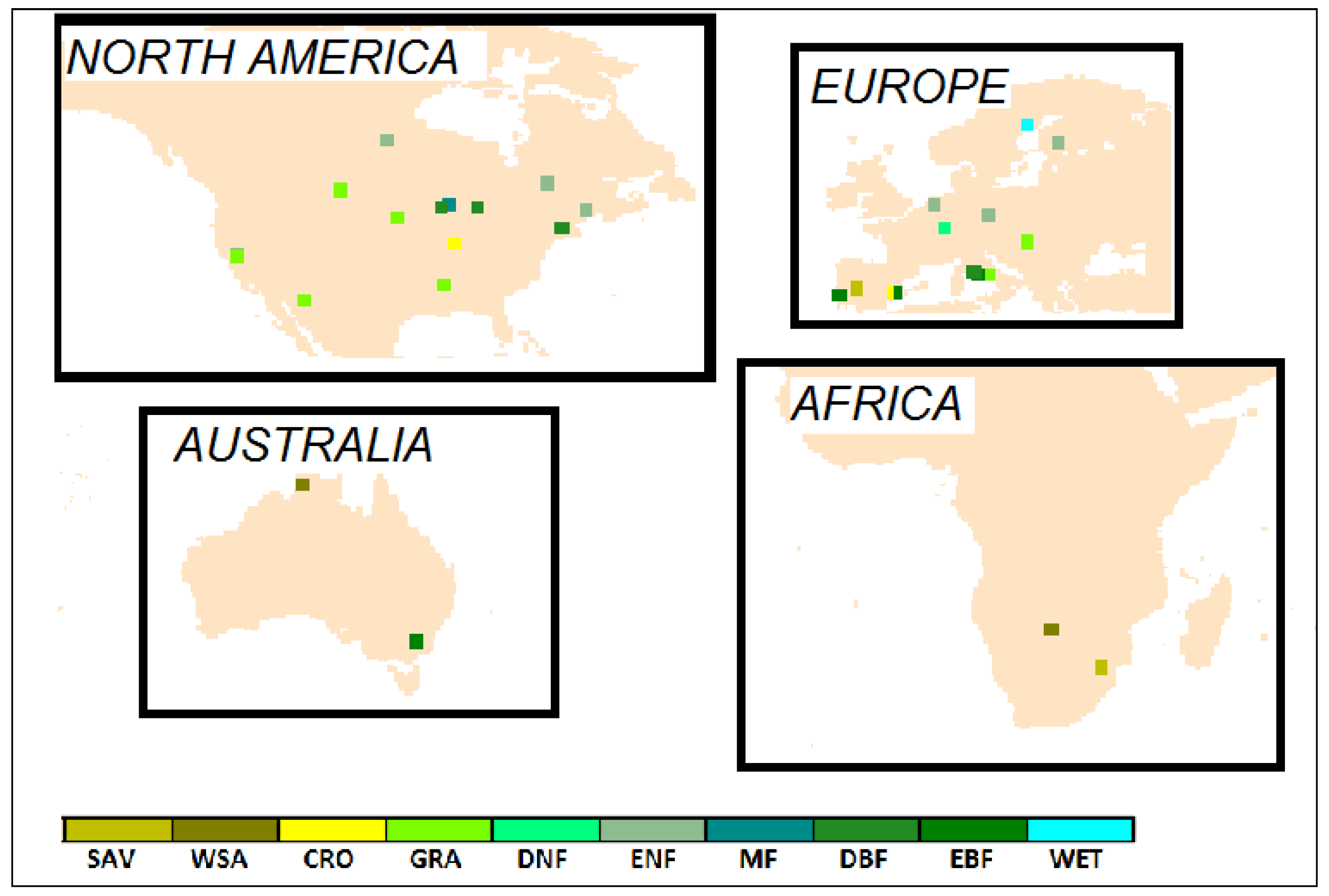
We use in situ observations of latent heat flux and meteorological variables (required to compute PET and identify dry periods, see Section 2.3) from eddy-covariance flux towers. The data were obtained through the Protocol for the Analysis of Land Surface Models (PALS; [32]) and come originally from the FLUXNET LaThuile free fair-use subset (fluxdata.org). Both flux and meteorological data have half-hourly temporal resolution, and we averaged them to a daily time step for this study in order to compare with the model daily data. Days where less than two-thirds of the half-hourly time steps were available for latent flux were neglected. Gap filling and quality control of the meteorological variables were previously conducted by PALS [33]. Figure 1 shows the spatial distribution and vegetation types of the sites used for this study, while

Table 1. Descriptive information about the 35 FLUXNET sites.

Site	Country	Latitude	Longitude	Vegetation Type	Period of Data
Amplero	Italy	41.90° N	13.61° E	Grassland	2003–2006
Audubon	United States	31.59° N	110.51° W	Grassland	2003–2005
Blodgett	United States	38.90° N	120.63° W	Evergreen Needleleaf	2000–2006
Bondville	United States	40.01° N	88.29° W	Cropland	1997–2006
Boreas	Canada	55.88° N	98.48° W	Evergreen Needleleaf	1997–2003
Brooking	United States	44.35° N	96.84° W	Grassland	2005–2006
Bugac	Hungary	46.69° N	19.60° E	Grassland	2003–2006
Castelporziano	Italy	41.71° N	12.38° E	Evergreen Broadleaf	2001–2006
Degero	Sweden	64.18° N	19.55° E	Permanent Wetland	2001–2005
El Saler	Spain	39.35° N	0.32° W	Evergreen Needleleaf	1999–2006
El Saler 2	Spain	39.28° N	0.32° W	Cropland	2005–2006
Espirra	Portugal	38.64° N	8.60° W	Evergreen Broadleaf	2002–2006
Fort Peck	United States	48.31° N	105.10° W	Grassland	2000–2006
Goodwin	United States	34.25° N	89.87° W	Grassland	2004–2006
Harvard	United States	42.54° N	72.17° W	Deciduous Broadleaf	1994–2001
Hesse	France	48.67° N	7.06° E	Deciduous Needleleaf	2001–2006
Howard	Australia	12.49° S	131.15° E	Woody Savanna	2002–2005
Howland	United States	45.20° N	68.74° W	Evergreen Needleleaf	1996–2004
Hyytiala	Finland	61.85° N	24.29° E	Evergreen Needleleaf	2001–2004
Kruger	South Africa	25.02° S	31.50° E	Savanna	2002–2003
Loobos	Netherlands	52.17° N	5.74° E	Evergreen Needleleaf	1997–2006
Majadas	Spain	39.94° N	5.77° W	Savanna	2004–2006
Mitra	Portugal	38.54° N	8.00° W	Evergreen Broadleaf	2005–2005
Mopane	Botswana	19.92° S	23.56° E	Woody Savanna	1999–2001
Quebecc	Canada	49.27° N	74.04° W	Evergreen Needleleaf	2002–2006
Quebecf	Canada	49.69° N	74.34° W	Evergreen Needleleaf	2004–2006
Rocca 1	Italy	42.41° N	11.93° E	Deciduous Broadleaf	2002–2006
Rocca 2	Italy	42.39° N	11.92° E	Deciduous Broadleaf	2004–2006
Sylvania	United States	46.24° N	89.35° W	Mixed Forest	2002–2005
Tharandt	Germany	50.96° N	13.57° E	Evergreen Needleleaf	1998–2005
Tonzi	United States	38.43° N	120.97° W	Woody Savanna	2002–2006
Tumba	Australia	35.66° S	148.15° E	Evergreen Broadleaf	2002–2005
Uni Michigan	United States	45.56° N	84.71° W	Deciduous Broadleaf	1999–2003
Vaira	United States	38.41° N	120.95° W	Grassland	2001–2006
Willow	United States	45.81° N	90.01° W	Deciduous Broadleaf	1999–2006

lists the 35 sites in total with some key information and periods available. The sites chosen each have at least one dry event (as defined in Section 2.3) in the time series and represent a global spread of climate and vegetation types.

2.2. Model Data

The model simulations that we evaluate here constitute the eartH2Observe project Water Resources Reanalysis 1 (WRR1) dataset, presented in Schellekens, et al. [34]. WRR1 consists of an ensemble of 10 GHM and LSM water cycle assessments, covering the period 1979–2012, that represents the state of the art in current global hydrological and land surface modeling. A list of the global models and some key information on their nature is given in

Table 2. Descriptive information about the 10 Water Resources Reanalysis 1 (WRR1) models. Evapotranspiration scheme as reported in Schellekens, et al. [34], where more detailed information on the WRR1 modelling protocol and different model process schemes is given. The groundwater interactions column refers to whether the groundwater is a dynamic reservoir and can interact with the unsaturated soil above through two-way fluxes (drainage and capillary rise). LSM—land surface model; GHM—global hydrological model; PET—potential evapotranspiration.

Model	Type	Time Step	Evapotranspiration Scheme	Soil Layers	Groundwater Interactions	References
HTESSEL-CaMa	LSM	1 h	Penman–Monteith	4	No	[36]
JULES	LSM	1 h	Penman–Monteith	4	No	[13,37]
ORCHIDEE	LSM	900 s	Bulk PET [38]	11	No	[39,40]
SURFEX-TRIP	LSM	900 s	Penman–Monteith	14	No	[41,42]
LISFLOOD	GHM	1 day	Penman–Monteith	2	No	[43]
PCR-GLOBWB	GHM	1 day	Hamon (tier 1) or imposed as forcing	1	Yes	[44,45,46]
SWBM	GHM	1 day	Inferred from net radiation	1	No	[47]
W3RA	GHM	1 day	Penman–Monteith	3	Yes	[48,49]
WaterGAP3	GHM	1 day	Priestley–Taylor	1	No	[50,51]
HBV-SIMREG	GHM	1 day	Penman, 1948	1	No	[52,53]

. GHMs typically operate at a one-day time step, whereas LSMs work at a shorter time step to allow for a representation and solution of the surface energy balance and the diurnal cycle. All 10 model simulations are driven by the same dataset; namely WATCH (WATer and global CHange) Forcing Data methodology applied to ERA-Interim reanalysis (WFDEI [35]), which provides three-hourly time intervals of the meteorological data that GHMs and LSMs typically use to run when they are uncoupled from atmospheric models (surface pressure, incoming radiation, wind speed, near surface humidity and temperature, and precipitation). The spatial resolution of the meteorological forcing data WFDEI and the WRR1 model outputs is 0.5°.

Benchmarking and signal-to-noise evaluations performed on WRR1 on the different components of the water cycle at the monthly timescale have reported large model uncertainty [34], and a summary of evaluation results on latent heat against flux tower observations is provided in Table S1. Here, we focus on a more process-based evaluation of models’ drydowns using daily ET (this is the highest temporal resolution available in WRR1 outputs). No calibration to better represent local conditions was performed by the models for this study, as we aim to evaluate the drydown model skill on large-scale applications such as WRR1.

2.3. Defining the Metric

We study drydowns during periods of no precipitation over vegetated areas. Therefore, to do so, we identify our drydowns by looking at the precipitation time series from the flux tower sites and from the model grids. We select periods of 10 or more days of no precipitation in order to have a sufficiently long time series for each drydown.

At the ET second stage, the ET ratio is typically assumed to have a linear dependency with the available soil moisture in the root zone [13,20], that is, as

$$\frac{ET\left(t\right)}{PET}=\frac{S\left(t\right)-S_w}{S_{cap}}$$

(1)

where $S\left(t\right)$ is the soil moisture storage in the root zone, $S_w$ is the soil moisture at wilting point in the root zone, $S_{cap}=S_{*}-S_w$ is the soil moisture capacity or maximum availability for transpiration in the root zone, and $S_{*}$ is the critical soil moisture in the root zone. All soil moisture variables in Equation (1) have units of m³ m⁻³. During this ET second stage of a drydown, there is no precipitation, runoff and drainage are negligible, and thus ET is the only process depleting the root zone soil moisture. The root zone soil water balance can be written as

$$\frac{dS\left(t\right)}{dt}=-ET\left(t\right)$$

(2)

Combining Equations (1) and (2) above, it follows that the ET ratio decays exponentially during the water-limited stage of a period of no precipitation, as

$$\frac{ET}{PET}=\frac{E{T}_0}{PE{T}_0}\exp \left(-\frac{t}{\mathsf{\tau }}\right)$$

(3)

where $E{T}_0/PE{T}_0$ is the ET ratio at t = 0, and $\mathsf{\tau }=S_{cap}/PET$. We define τ (days) as the lifetime of a drydown, a physical parameter with units of time that characterises the drydown as a function of the root system of the site/area and the event evaporative demand from the atmosphere. The τ parameter is independent of the initial ET ratio, and thus independent of the initial state of soil moisture when the precipitation stops. A similar exponential curve has been derived and used previously in other studies using observed and simulated time series of ET, for example, the works of [7,31]. However, we have adopted the use of an ET ratio, helping the identification of water-limited drydowns as those events with an ET ratio below one.

The method only works when the soil reaches water-limited conditions. To enable this, we introduce a threshold and define a ‘dry event’ as an event with $0<\mathsf{\tau }<50$ days. This threshold indicates that events that take 34 days or more to decrease the ET ratio to a half of its initial value are excluded from the analysis. Such excluded events present very slow drying or no drying at all, which can be the result of no shortage of root zone soil moisture in regions of shallow groundwater table and slow drainage [54], artificial water sourced from irrigation [55], or low radiation supply in winter. We also consider the first day of no precipitation as the starting point of the drydown event. This decision avoids including interception (a process that does not evaporate soil water, but canopy intercepted water) in the water-limited ET, thus effectively assuming that any water intercepted by vegetation is evaporated within 24 h [26]. These constraints are designed to ensure that all the drydowns analysed use data from the ET second stage, and any conclusion drawn from our analysis will be valid for water-limited conditions.

The calculation of PET was performed following the Penman–Monteith approach [56], which includes the effect of stomatal resistance to calculate PET from atmospheric conditions of temperature, wind, incoming radiation, and humidity (as discussed in Robinson, et al. [57]). We specifically used the same parameters as in Equation (4) of the cited paper [57], for a reference crop of 0.12 m height and stomatal resistance of 70 s/m and, therefore, note that it will be biased in winter, as well as for tree sites.

We calculate τ for each drydown using the non-linear least squares interpolation to fit the data to an exponential function in time of the form $y=a\times exp\left(-b\times t\right)$, where y is the time series of daily ET/PET, t is time (days of the dry period), and τ is diagnosed as $\mathsf{\tau }=1/b$.

We are looking to evaluate the response of a landscape to dry periods. Given that we are only considering water-limited conditions, we assign a single drydown exponential curve to all drydown events at a particular site/grid cell. We use the median τ to characterise the landscape. The assumption that a single drydown metric for a particular site/grid cell is valid is tested by calculating the interquartile range.

2.4. Applying the Metric to the Flux Tower Data

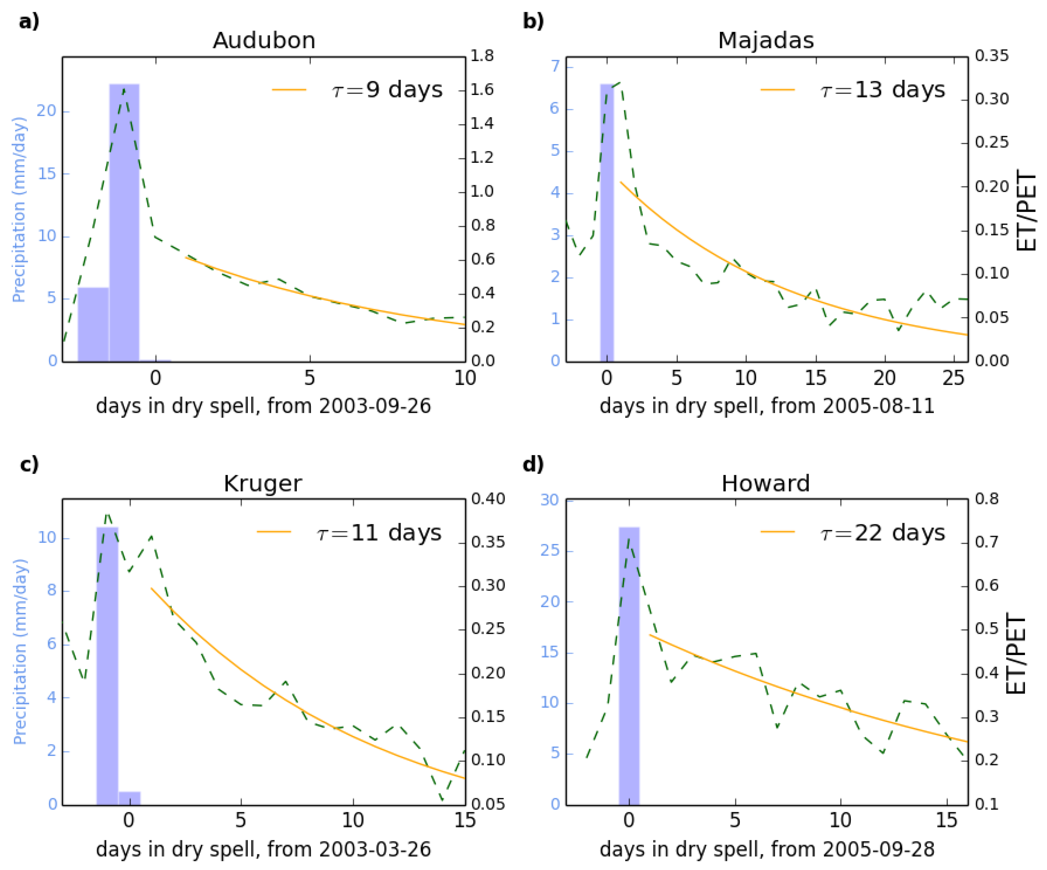
We used the in situ measurements of meteorological variables to calculate PET for the observation sites. As a showcase of the methodology, Figure 2 presents four exemplary drydowns identified and analysed from the sites that presented a highest number of dry events per year in their continental area (Audubon in United States, Majadas in Spain, Kruger in South Africa, and Howard in Australia). As a measurement of the tightness of the linear relationship between ET ratio and root zone soil moisture during drydowns, we use the standard deviation error (σ) of the fitting. For the events in Figure 2, σ metrics are given in the caption.

2.5. Applying the Metric to the Models

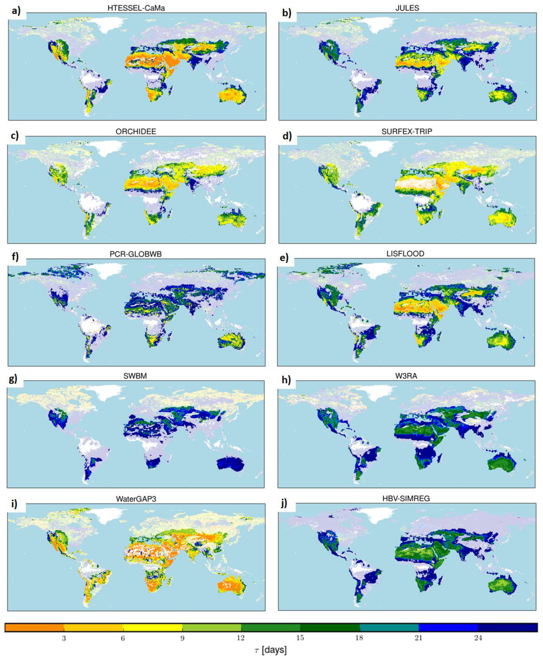
For the models, we calculated a common PET using the WFDEI meteorological dataset that drives all WRR1. We then calculated the drydown metric over the full dataset. Figure 3 shows the median τ values calculated at every grid cell for the 34 year runs of the WRR1 models. This is discussed in Section 4.3.

3. Results

3.1. Site Level Results and Selection of Representative Sites

The observed median lifetime τ characterizing drydowns for the observation sites, as well as the fraction of events of 10 or more days of no precipitation that fall under our definition of dry event, are shown in

Table 3. Results of the drydown median lifetimes (τ) and fraction of dry events at the FLUXNET observation sites that present at least one dry event in the available dataset. N_dry is the number of dry events identified and N_total is the total number of events with 10 or more days of no precipitation. The sites are sorted in order of increasing fraction of events identified as dry events (N_dry/N_total ≥ 0.5). IQR is the interquartile range of drydown lifetimes distribution for dry events identified in the observations. “--” means that the IQR is non-applicable for sites with only 1 dry event.

Site	τ [d]	Ndry	IQR [d]	Ndry/Ntotal
Blodgett	14.2	1	--	0.04
Hyytiala	40.8	1	--	0.09
Degero	45	1	--	0.09
Boreas	32.9	1	--	0.11
Harvard	23.1	1	--	0.13
Uni Michigan	12.4	1	--	0.13
El Saler 2	34.6	2	2.5	0.13
Brooking	14.2	1	--	0.14
Quebecc	8.1	1	--	0.17
Howlandm	33.3	2	15.2	0.18
Tumba	37.6	2	7.6	0.18
Castel	38.0	2	10.6	0.18
El Saler	29.3	7	8.9	0.2
Rocca 2	35.8	2	3.1	0.22
Willow	17.9	3	3.9	0.23
Amplero	17.6	1	--	0.25
Espirra	28.6	3	6.8	0.25
Goodwin	19.2	2	4.6	0.25
Quebecf	16.8	2	8.2	0.29
Howard	25.5	4	10.2	0.33
Fort Peck	10.9	8	16.4	0.35
Rocca 1	30.5	7	6.0	0.37
Mitra	35.8	3	3.6	0.38
Sylvania	17.9	2	5.6	0.4
Bugac	28.5	3	8.5	0.43
Loobos	16.2	5	6.2	0.45
Hesse	23.4	5	4.7	0.5
Bondville	18.2	10	15.2	0.5
Tonzi	27.1	12	32.2	0.5
Vaira	16.8	13	5.2	0.54
Majadas	18.4	11	16.1	0.58
Mopane	24.7	12	14.3	0.75
Tharandt	29.2	4	13.4	0.8
Kruger	18.4	9	8.5	0.82
Audubon	9.1	16	8.4	0.94

.

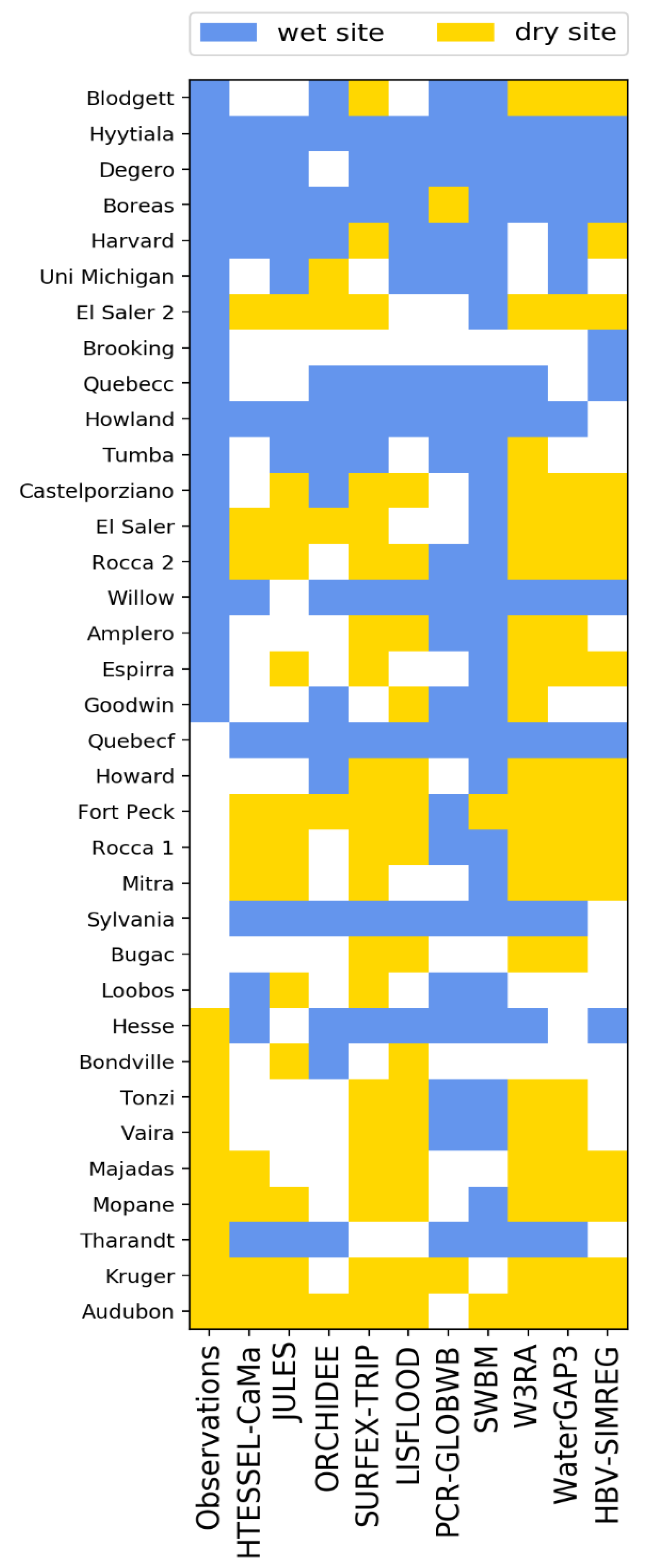
In addition, Figure 4 shows the identification of the sites as dry (50% or more of the events at the site are dry events) or wet (25% or less of the events at the site are dry). We used the flux tower data for observations (first column) and the modeled data for the 10 WRR1 models at the grid cells containing the sites locations (rest of the columns). A study of these results shows that the sites fall into one of three categories:

• Too wet for analysis.
• Observations are too wet, but models are dry enough.
• Both observations and models are dry enough.

Eighteen sites fall into categories 1 or 2. They are found to be wet by the observations (N_dry/N_total ≤ 0.25; top sites in Figure 4). However, we can retrieve very useful information in terms of model representation, as the models do not agree in finding some of the locations to be wet (seven sites are in category 2). This is discussed in Section 4.4.

Category 3 includes the sites that can be used for subsequent analysis. On sites with a higher number of dry events and that are found to be dry by observations and by most models (e.g., Tonzi, Vaira, Majadas, Mopane, Kruger, Audubon), a comparison of observed and modeled drydown characteristics is more comprehensive and significant, providing information about drought response by the land in both observations and models.

The σ metric for all dry events identified at the observation sites by the flux data and by the models is consistently low (see Figure S1) and has no apparent correlation with the ET/PET decrease during the drydown. This weak relationship indicates that the severity of the drydown and/or its duration (factors affecting the decrease in ET ratio) do not have a strong effect on the tightness of the exponential fitting, further supporting the exponential curve assumption for ET/PET decay during drydowns under water-limited conditions.

3.2. Analysis of Results at the Site Level

Table 4. Results of the drydown median lifetimes (τ [d]) at the 10 FLUXNET sites with higher number of dry events identified and at the grid cells containing the site locations in the WRR1 models. The entries are sorted in order of decreasing τ in the observations. The values given here and their corresponding interquartile range are plotted in Figure 5. The number of dry events in the observations is shown in Table 3, and the number of dry events in the models (not shown here) is greater than that in the observations given the larger data record (34 years).

Site	Observations	HTESSEL-CaMa	JULES	ORCHIDEE	SURFEX-TRIP	LISFLOOD	PCR-GLOBWB	SWBM	W3RA	WaterGAP3	HBV-SIMREG
Rocca 1	30.5	18.7	20.7	25.0	14.1	16.6	30.7	42.4	19.0	15.6	22.9
El Saler	29.3	8.7	18.7	15.7	11.7	24.6	31.9	24.6	17.6	9.2	24.5
Tonzi	27.1	25.4	34.5	24.3	22.8	27.4	37.9	27.1	24.5	17.8	38.0
Mopane	24.7	5.2	14.1	16.3	10.2	16.7	5.9	33.1	22.3	13.9	15.2
Majadas	18.4	22.2	30.1	22.0	13.2	18.8	9.7	32.3	16.5	18.0	23.6
Kruger	18.4	19.0	26.7	18.7	14.0	25.6	31.5	28.8	29.1	12.2	35.6
Bondville	18.2	26.8	24.9	26.9	16.2	17.9	29.9	26.7	27.3	14.3	26.6
Vaira	16.8	25.4	34.5	24.3	22.8	27.4	37.9	27.1	24.5	17.8	38.0
Fort Peck	10.9	11.8	16.3	9.1	7.5	19.5	28.6	16.7	15.7	8.2	19.1
Audubon	9.1	14.0	19.7	9.5	12.3	19.7	19.5	25.8	19.3	8.4	20.0

and Figure 5 show the computed median τ for observations and all 10 WRR1 models on sites where higher number of dry events are observed (using the threshold of seven events here, see Table 3), ordered from highest to lowest observed τ.

In addition to the median τ and its interquartile range for observed and modeled dry events (bar chart inside each plot), Figure 5 represents the hypothetical drydown characterizing each site (orange dash lines for observations and solid color lines for models), following an exponential curve from an ET ratio of 1.0 at the initial day of the dry spell, with a lifetime parameter equal to the median τ. This representation of hypothetical drydowns gives an illustrative idea of the rate of drying represented by observations and models at each site. For these 10 sites in Figure 5, we see a strong model variability. Some features are common to most sites: JULES (yellow) is the slowest (highest τ) of the LSMs, SURFEX-TRIP (red) is the quickest (lowest τ) of the LSMs, and WaterGAP3 (brown) is the quickest model. Across sites, there is greater consistency between the LSM responses than is found between the GHM responses.

The mismatch between modeled and observed drydowns in Figure 5 can be explained, in part, by the locality of the flux tower measurements. As observations have a footprint typically below 10 km² [58], and given the integrative nature of global models that work at a spatial scale resolution of thousands of km² (like WRR1 models; spatial resolution of 0.5°), the vegetation ‘type’ of the flux tower might not match that of the modeled grid cell [34].

The mismatch between the modeled vegetation and observations can easily be seen in Figure 5a–d. The models clearly represent drydown rates much better at Tonzi, with six models having a value of median τ within 17% of the observations. However, at the other three sites, most models consistently overestimate the drydown rates (lower lifetimes), meaning that the soil dries quicker in the models than in the observations. In all of these cases, the flux towers and models disagree in the land cover (

Table 5. Vegetation type at the 10 FLUXNET sites with higher number of dry events identified and dominant plant functional type at the grid cells containing the site locations in the WRR1 models. The plant functional types (PFT) given here correspond to the dominant type (highest fractional cover in the grid cell) in the vegetation cover data used by the JULES model (from data derived from the International Geosphere-Biosphere Programme: http://www.igbp.net/).

Site	Site Vegetation Type	Grid Cell Dominant PFT
Rocca 1	Deciduous Broadleaf	Shrubs
El Saler	Evergreen Needleleaf	Grasses
Tonzi	Woody Savanna	Broadleaf Trees
Mopane	Woody Savanna	Grasses
Majadas	Savanna	Grasses
Kruger	Savanna	Grasses
Bondville	Cropland	Grasses
Vaira	Grassland	Broadleaf Trees
Fort Peck	Grassland	Grasses
Audubon	Grassland	Grasses

); with flux towers saying they are tree based and models saying they are grasses (El Saler and Mopane), or flux towers saying broadleaf trees while the models say shrubs (Rocca 1).

The opposite situation occurs at the Vaira site (Figure 5h), where all models underestimate the drydown rates (higher lifetimes), explained in this case by a vegetation cover mismatch in the other direction; grassland at the site and broadleaf trees as dominantly seen by the models (Table 5). At the sites with grass as vegetation cover for both the observation site and the models (Fort Peck and Audubon; Figure 5i,j), the model drydown underestimation is not as widespread and some models (HTESSEL-CaMa, ORCHIDEE, SURFEX-TRIP, WaterGAP3) capture low drydown rates (quick drying).

3.3. Generalizing the Results for Model Evaluation

It is clear that vegetation type is an important factor in the drydown metric, as the order of the sites in Table 4 from high to low drydown rates corresponds with decreasing vegetation stature (Table 5). To create a generic metric, we thus aggregate the drydown events according to the vegetation cover at their site or dominant in their model grid cell (Figure S2), enabling a more like-for-like comparison. This allows us to use the whole global dataset in the case of the models, and reach a comprehensive characterization of modeled drydown rates.

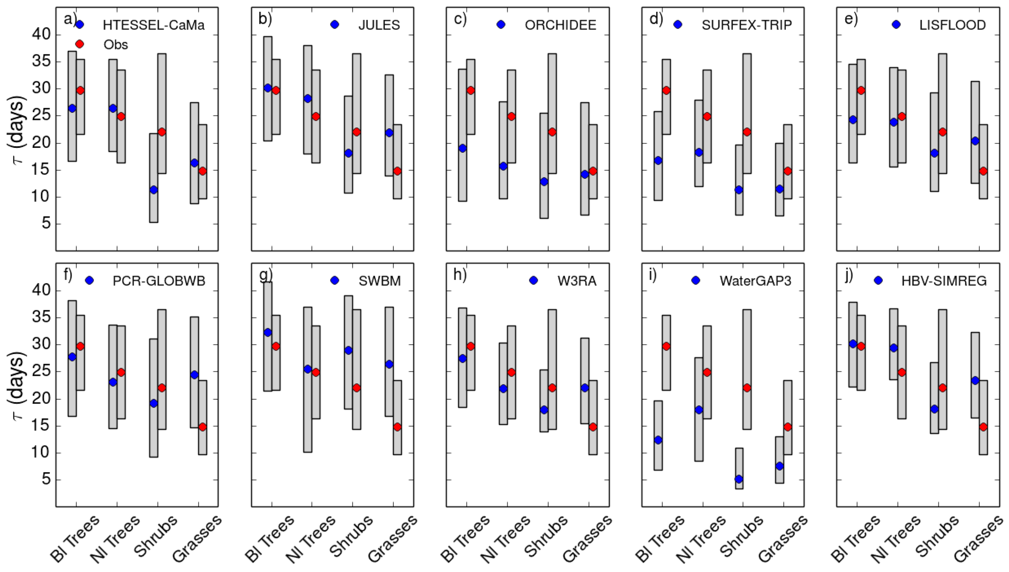
In Figure 6, we plot the resulting drydown metric for the four vegetation types in Figure S2 across all climates for all the models. Alongside is the metric from the observations. The relation is very apparent and almost linear in the case of observations, from slowest drying over broadleaf trees (τ~30 d), then needleleaf trees (τ~25 d), and shrubs (τ~22 d), to quick drying over grasses (τ~20 d). Most models show a similar decrease in median τ from broadleaf trees to grasses, with the exception of the rates for shrubs, where the models (all but SWBM) present quicker rates than those for grasses. This might be explained by the models assuming that shrublands are sparse (low leaf area indexes, low canopy heights, and shallow roots), whereas the flux sites that are categorised as ‘shrub’ tend to represent zones more intensely vegetated (i.e., the Tonzi site reports an overstory of blue oak trees covering 40% of the total vegetation, with intermittent grey pine trees and understory species including a variety of grasses and herbs [59]).

4. Discussion

Global model outputs like the WRR1 product analysed here tend to be evaluated using earth observation datasets for a characterization of the model skill to reproduce observed global or regional water budgets (for example, see the works of [34,36]), whereas flux tower data can be used to evaluate the model surface fluxes exchange (for example, see the work of [60]). In this work, using flux tower data, we look for a process based evaluation that helps characterise the models in their capability to predict drought responses, and thus provide useful information to both model developers that are constantly working to improve the tools and water managers or other potential users of WRR1 that might be interested in drought response over particular regions. The reasons for the accuracy or shortcomings of the WRR1 models in their simulation of water-limited drydowns, however, will be dependent on particular model configurations and process representations (for instance, only two models incorporate groundwater interactions with the unsaturated zone in the soil).

4.1. Role of Vegetation in τ

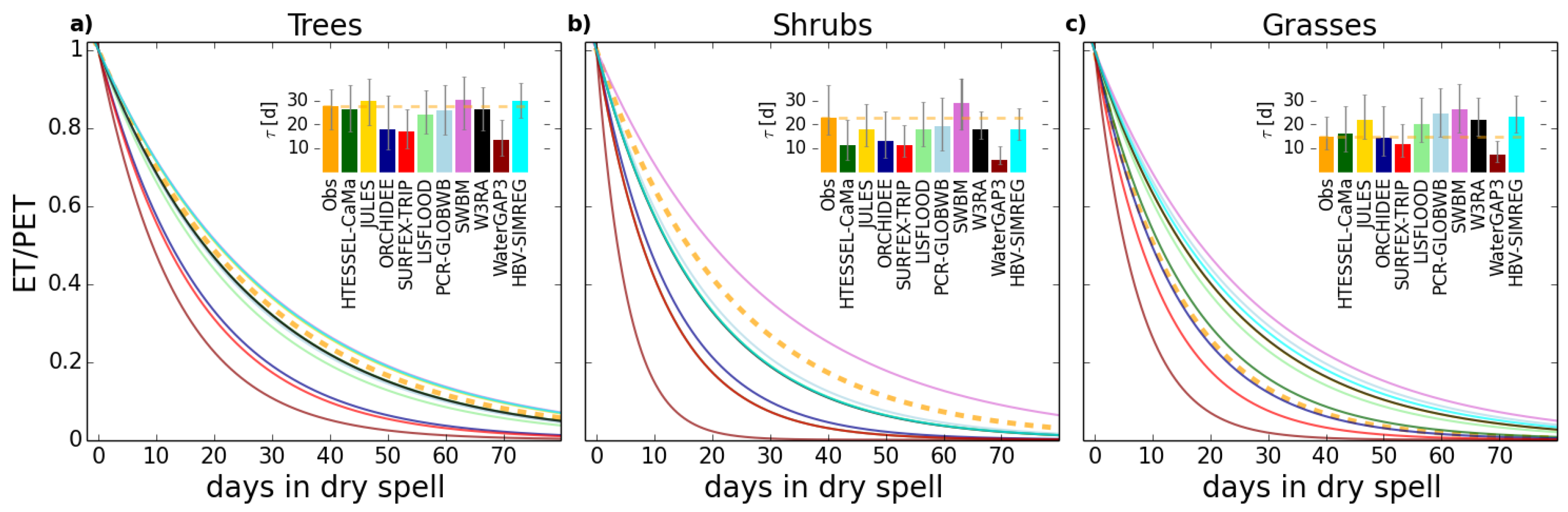
The analysis in Section 3 shows a strong link between drydown and vegetation cover. We can simplify our analysis to a first order vegetation cover differences using a three-type classification: trees, shrubs, and grasses. For the models, we use the dominant vegetation type map (Figure S2) to identify any event over tree dominated regions (broadleaf trees, needleleaf trees), shrub dominated regions, and grass dominated regions. For the observation sites, we classify sites with vegetation cover reported of “Grasslands” or “Croplands” (Table 1) as grasses, “Savannah” or “Woody savannah” as shrubs, and the rest of the sites as trees. Under this criterion, we have a simpler characterization of drydown rates by both models and observations (Figure 7). As discussed in Section 3.3, there is an issue with shrubs as the models dry too quickly (Figure 7b), with SWBM being the only model slower than observations (higher τ). Focusing on trees and grasses (Figure 7a,c), we can see that the models represent better the drydown rates over tree covered regions (six models within 10% of observed median τ: 27.8 days), whereas over grass covered regions, the model variability and differences with observations are higher (only two models, HTESSEL-CaMa and ORCHIDEE, within 10%).

The observations show a reduction in median τ from trees to grasses of 47% (from 27.8 to 14.8 days). However, as shown in

Table 6. Results of the drydown median lifetimes (τ [d]) for tree and grass covers. The third row is calculated as follows: 100—(second row/first row) × 100. The data in the first and second row reflect values shown in Figure 7a,c.

	Observations	HTESSEL-CaMa	JULES	ORCHIDEE	SURFEX-TRIP	LISFLOOD	PCR-GLOBWB	SWBM	W3RA	WaterGAP3	HBV-SIMREG
Trees	27.8	26.4	29.7	18.1	17.1	24.2	25.8	30.1	26.3	13.4	29.9
Grasses	14.8	16.2	21.9	14.2	11.6	20.3	24.5	26.5	22.0	7.5	23.3
% decrease	47	38	26	21	32	16	5	12	16	44	22

, the models show a smaller reduction depending on whether they are LSMs (between 21% and 38%) or GHMs (22% or below, with the exception of WaterGAP3, which presents very quick drydown rates for all vegetated areas). HTESSEL-CaMa shows this reduction with very good agreement with observations for both trees and grasses. Other two LSMs, ORCHIDEE and SURFEX-TRIP, which are significantly quicker than observations over trees, present a much better agreement over grasses. JULES shows a very good agreement with observations for trees (29.7 days versus 27.8 days in the observations), but the τ reduction for grasses is too small. SWBM also shows very good agreement with observations for trees (30.1 days), but then the representation of grasses is highly overestimated with a median τ of 26.5 days versus 14.8 days in the observations (too little reduction of τ from trees to grasses).

4.2. Other Factors

We acknowledge that the soil texture and not only the vegetation type should explain part of the observed and modelled variance of the drydown rates, as it determines the soil capacity to hold and conduct water at the surface and through the root zone (i.e., sandy soils with larger pores and lower water suction will evapotranspirate more easily and have quicker drainage down the soil column). This was shown by a clear systematic decrease of drydown rates with sand fraction by McColl, et al. [20] when they analysed surface soil moisture drying. However, when we relate our global modeled data of drydown rates (using ET ratio) with soil water suction data from the Harmonized World Soil Database (HWSD [61]), we do not find a relationship as clear among models as the results show when relating drydown rates with vegetation type (Figure S3).

4.3. Global Maps of Median τ

Our methodology provides global maps of median τ from the WRR1 models, shown in Figure 3. Some of the features are robust with conclusions already drawn from the analysis at the site level and by plant functional types: (1) LSMs (Figure 3a–d) present very similar spatial patterns with SURFEX-TRIP drying quicker than the rest and JULES slower; (2) GHMs (Figure 3e–j) present overall slower drying than LSMs and higher model variability; (3) the within model variability in spatial patterns is more apparent in LSMs pointing at different characterization depending on land cover; and (4) WaterGAP3 is a quick outlier.

These maps may be useful way to compare the features of the different models and to use satellite data for evaluation.

4.4. Identification of Drydowns and Characterization of Sites

The identification of water-limited drydowns detailed in Section 2.3 is a departure from recent studies where the drydown evaluation had to be discretised in bins of antecedent rainfall [28,30]. In addition to the main purpose of this work of evaluating how quickly drydowns occur when the soil water limitation affects surface fluxes, we have used our drydown identification method to characterise sites/regions as dry or wet, considering the ratio of periods of no precipitation that fall on our ‘dry event’ definition.

A group of sites (Blodgett, El Saler, El Saler 2, Castelporziano, Rocca 2, Amplero, and Espirra) were found to be dry by most models, but considered wet by the observations (Figure 4), even when they were located over semiarid regions, meaning that the models somehow stressed evaporative fluxes during periods of no precipitation, even though such stress was not observed. This points to other model processes being responsible for the observation/model mismatch in the identification of sites as dry, rather than the rate of drying, like irrigation (case of El Saler 2) or intensified soil moisture memory due to shallow groundwater connectivity [62]. Three of these sites (Blodgett, Amplero, and Espirra) were used by Ukkola, et al. [55] to analyse a range of LSMs (JULES and ORCHIDEE included) in their representation of droughts. These authors concluded that the models overestimate intensity and duration, falling in agreement with our findings here. We note that two particular GHMs (PCR-GLOBWB and SWBM) do not find these locations to be dry, however, these models tend to characterise all sites as wet.

Other sites were characterised as wet by both observations and models, as they are located in wet and cold northern latitudes (Hyytiala, Boreas, Degero, Quebecc) or under all year long humid climate conditions (Tumba, Willow).

Therefore, even though other processes beyond soil drying under water-limited conditions, like groundwater connectivity to the root zone, are not within the scope of this analysis as the theory does not hold on such conditions, the simple identification of dry/wet sites already gives some answers to the questions of what sites are actually water-limited during no precipitation periods and whether the models agree with observations in this identification.

4.5. On the Methodolody

We acknowledge that the assumption of constant PET during the dry event is a condition in order to obtain Equation (3). Possible oscillations of PET from day to day should be minimal during a dry period, and we have calculated ET/PET on a daily time step, so such oscillations are expected to be smoothed out on the exponential decay adjustment. Further, the restriction to the methodology of only considering events with 0 < τ < 50 days will neglect possible events where PET variations might result in the inaccuracy of the method.

Following this work, but slightly out of the scope of this publication, we consider separating events, for a particular site/region, into different PET categories. This would give us further insights into understanding under what atmospheric conditions the models represent more/less accurately the drydown process.

5. Summary and Conclusions

In this paper, we study the concept that we can characterise the rate of drydown after a rainfall event as a single value, and whether this is a useful metric to evaluate models. We set out to investigate if such a key quantity could be extracted from several years of direct measurements and whether existing large-scale models have a fixed value of this metric in time.

Ideally, we would be able to observe this quantity from satellite observations so that we could obtain global maps. However, there are problems with the use of satellite soil moisture observations to study this, as only the top surface soil moisture can be seen. In order to overcome the observed soil moisture limitations, other studies have focused on the surface responses rather than the actual soil moisture evolution, for instance, analyzing the energy balance response through warming rates of the land surface, using a methodology based on satellite land surface temperature products [28,30]. In this study, however, we use the most direct observation of evapotranspiration—the eddy-covariance method, commonly referred to as flux tower measurements.

The study reveals that it is possible to quantify the drydown process using the exponential curve of decrease of evapotranspiration (normalised by the evaporative demand or potential evaporation) when we have daily data of evapotranspiration, potential evapotranspiration, and precipitation. We define the lifetime parameter τ of this curve as our drydown metric, and characterise the land using the median τ obtained for all dry events identified within the time series of data available. A comparison of 35 sites showed a marked relation between the vegetation cover at the site and the drydown rates, with tree sites drying slower than grassland sites because of differences in the root system, and thus the soil water that they can reach.

We quantify the drydown metric for a suite of global land surface and hydrological models from the WRR1 assessment [34] run globally at 0.5° resolution and compare it to the results from flux tower data. We find that a large part of the disagreement between the modeled and observed metric comes from discrepancies in the land cover type specified by the models compared with the actual vegetation at the flux tower. When we group the modeled metric into vegetation cover characterizations, we obtain a more robust metric for the models that correlates well with the findings at the site level. Land surface models show a strong difference between trees and grasses, in agreement with observations, while most large-scale hydrology models show a markedly lower difference.

We conclude that flux tower data can be used to evaluate drydown processes in global models using the median lifetime parameter τ, which is a property of the land and hence independent of the precipitation forcing, as long as the vegetation cover at the sites and in the models is taken into account.

References

- Seneviratne, S.I.; Corti, T.; Davin, E.L.; Hirschi, M.; Jaeger, E.B.; Lehner, I.; Orlowsky, B.; Teuling, A.J. Investigating soil moisture–climate interactions in a changing climate: A review. Earth-Sci. Rev. 2010, 99, 125–161. [Google Scholar] [CrossRef]
- Botter, G.; Peratoner, F.; Porporato, A.; Rodriguez-Iturbe, I.; Rinaldo, A. Signatures of large-scale soil moisture dynamics on streamflow statistics across U.S. climate regimes. Water Resour. Res. 2007, 43. [Google Scholar] [CrossRef] [Green Version]
- Clark, M.P.; Fan, Y.; Lawrence, D.M.; Adam, J.C.; Bolster, D.; Gochis, D.J.; Hooper, R.P.; Kumar, M.; Leung, L.R.; Mackay, D.S.; et al. Improving the representation of hydrologic processes in Earth System Models. Water Resour. Res. 2015, 51, 5929–5956. [Google Scholar] [CrossRef] [Green Version]
- McColl, K.A.; Alemohammad, S.H.; Akbar, R.; Konings, A.G.; Yueh, S.; Entekhabi, D. The global distribution and dynamics of surface soil moisture. Nat. Geosci. 2017, 10, 100–104. [Google Scholar] [CrossRef]
- Miguez-Macho, G.; Fan, Y. The role of groundwater in the Amazon water cycle: 1. Influence on seasonal streamflow, flooding and wetlands. J. Geophys. Res. Atmos. 2012, 117. [Google Scholar] [CrossRef] [Green Version]
- Rosenzweig, C.; Tubiello, F.N.; Goldberg, R.; Mills, E.; Bloomfield, J. Increased crop damage in the US from excess precipitation under climate change. Glob. Environ. Change 2002, 12, 197–202. [Google Scholar] [CrossRef] [Green Version]
- Teuling, A.J.; Seneviratne, S.I.; Williams, C.; Troch, P.A. Observed timescales of evapotranspiration response to soil moisture. Geophys. Res. Lett. 2006, 33. [Google Scholar] [CrossRef] [Green Version]
- Koster, R.D.; Suarez, M.J. Soil Moisture Memory in Climate Models. J. Hydrometeorol. 2001, 2, 558–570. [Google Scholar] [CrossRef] [Green Version]
- Lorenz, R.; Jaeger, E.B.; Seneviratne, S.I. Persistence of heat waves and its link to soil moisture memory. Geophys. Res. Lett. 2010, 37. [Google Scholar] [CrossRef] [Green Version]
- Taylor, C.M.; de Jeu, R.A.M.; Guichard, F.; Harris, P.P.; Dorigo, W.A. Afternoon rain more likely over drier soils. Nature 2012, 489, 423–426. [Google Scholar] [CrossRef] [Green Version]
- Prudhomme, C.; Giuntoli, I.; Robinson, E.L.; Clark, D.B.; Arnell, N.W.; Dankers, R.; Fekete, B.M.; Franssen, W.; Gerten, D.; Gosling, S.N.; et al. Hydrological droughts in the 21st century, hotspots and uncertainties from a global multimodel ensemble experiment. Proc. Natl. Acad. Sci. USA 2014, 111, 3262–3267. [Google Scholar] [CrossRef]
- Koster, R.D.; Guo, Z.; Yang, R.; Dirmeyer, P.A.; Mitchell, K.; Puma, M.J. On the Nature of Soil Moisture in Land Surface Models. J. Clim. 2009, 22, 4322–4335. [Google Scholar] [CrossRef] [Green Version]
- Best, M.J.; Pryor, M.; Clark, D.B.; Rooney, G.G.; Essery, R.L.H.; Ménard, C.B.; Edwards, J.M.; Hendry, M.A.; Porson, A.; Gedney, N.; et al. The Joint UK Land Environment Simulator (JULES), model description—Part 1: Energy and water fluxes. Geosci. Model Dev. 2011, 4, 677–699. [Google Scholar] [CrossRef]
- Famiglietti, J.S.; Ryu, D.; Berg, A.A.; Rodell, M.; Jackson, T.J. Field observations of soil moisture variability across scales. Water Resour. Res. 2008, 44. [Google Scholar] [CrossRef]
- Entekhabi, D.; Njoku, E.G.; O’Neill, P.E.; Kellogg, K.H.; Crow, W.T.; Edelstein, W.N.; Entin, J.K.; Goodman, S.D.; Jackson, T.J.; Johnson, J.; et al. The Soil Moisture Active Passive (SMAP) Mission. Proc. IEEE 2010, 98, 704–716. [Google Scholar] [CrossRef]
- Kerr, Y.H.; Waldteufel, P.; Richaume, P.; Wigneron, J.P.; Ferrazzoli, P.; Mahmoodi, A.; Bitar, A.A.; Cabot, F.; Gruhier, C.; Juglea, S.E.; et al. The SMOS Soil Moisture Retrieval Algorithm. IEEE Trans. Geosci. Remote Sens. 2012, 50, 1348–1403. [Google Scholar] [CrossRef]
- Liu, Y.Y.; Dorigo, W.A.; Parinussa, R.M.; de Jeu, R.A.M.; Wagner, W.; McCabe, M.F.; Evans, J.P.; van Dijk, A.I.J.M. Trend-preserving blending of passive and active microwave soil moisture retrievals. Remote Sens. Environ. 2012, 123, 280–297. [Google Scholar] [CrossRef]
- Albergel, C.; de Rosnay, P.; Gruhier, C.; Muñoz-Sabater, J.; Hasenauer, S.; Isaksen, L.; Kerr, Y.; Wagner, W. Evaluation of remotely sensed and modelled soil moisture products using global ground-based in situ observations. Remote Sens. Environ. 2012, 118, 215–226. [Google Scholar] [CrossRef]
- Champagne, C.; Rowlandson, T.; Berg, A.; Burns, T.; L’Heureux, J.; Tetlock, E.; Adams, J.R.; McNairn, H.; Toth, B.; Itenfisu, D. Satellite surface soil moisture from SMOS and Aquarius: Assessment for applications in agricultural landscapes. Int. J. Appl. Earth Obs. Geoinf. 2016, 45, 143–154. [Google Scholar] [CrossRef] [Green Version]
- McColl, K.A.; Wang, W.; Peng, B.; Akbar, R.; Short Gianotti, D.J.; Lu, H.; Pan, M.; Entekhabi, D. Global characterization of surface soil moisture drydowns. Geophys. Res. Lett. 2017, 44, 3682–3690. [Google Scholar] [CrossRef]
- Shellito, P.J.; Small, E.E.; Colliander, A.; Bindlish, R.; Cosh, M.H.; Berg, A.A.; Bosch, D.D.; Caldwell, T.G.; Goodrich, D.C.; McNairn, H.; et al. SMAP soil moisture drying more rapid than observed in situ following rainfall events. Geophys. Res. Lett. 2016, 43, 8068–8075. [Google Scholar] [CrossRef] [Green Version]
- Shellito, P.J.; Small, E.E.; Livneh, B. Controls on surface soil drying rates observed by SMAP and simulated by the Noah land surface model. Hydrol. Earth Syst. Sci. 2018, 22, 1649–1663. [Google Scholar] [CrossRef] [Green Version]
- Ghannam, K.; Nakai, T.; Paschalis, A.; Oishi, C.A.; Kotani, A.; Igarashi, Y.; Kumagai, T.O.; Katul, G.G. Persistence and memory timescales in root-zone soil moisture dynamics. Water Resour. Res. 2016, 52, 1427–1445. [Google Scholar] [CrossRef] [Green Version]
- Orth, R.; Seneviratne, S.I. Analysis of soil moisture memory from observations in Europe. J. Geophys. Res. Atmos. 2012, 117. [Google Scholar] [CrossRef] [Green Version]
- Dirmeyer, P.A.; Wu, J.; Norton, H.E.; Dorigo, W.A.; Quiring, S.M.; Ford, T.W.; Santanello, J.A., Jr.; Bosilovich, M.G.; Ek, M.B.; Koster, R.D.; et al. Confronting Weather and Climate Models with Observational Data from Soil Moisture Networks over the United States. J. Hydrometeorol. 2016, 17, 1049–1067. [Google Scholar] [CrossRef]
- Blyth, E.; Harding, R.J. Methods to separate observed global evapotranspiration into the interception, transpiration and soil surface evaporation components. Hydrol. Process. 2011, 25, 4063–4068. [Google Scholar] [CrossRef]
- Laio, F.; Porporato, A.; Ridolfi, L.; Rodriguez-Iturbe, I. Plants in water-controlled ecosystems: Active role in hydrologic processes and response to water stress: II. Probabilistic soil moisture dynamics. Adv. Water Resour. 2001, 24, 707–723. [Google Scholar] [CrossRef]
- Harris, P.P.; Folwell, S.S.; Gallego-Elvira, B.; Rodríguez, J.; Milton, S.; Taylor, C.M. An Evaluation of Modeled Evaporation Regimes in Europe Using Observed Dry Spell Land Surface Temperature. J. Hydrometeorol. 2017, 18, 1453–1470. [Google Scholar] [CrossRef]
- Folwell, S.S.; Harris, P.P.; Taylor, C.M. Large-Scale Surface Responses during European Dry Spells Diagnosed from Land Surface Temperature. J. Hydrometeorol. 2016, 17, 975–993. [Google Scholar] [CrossRef]
- Gallego-Elvira, B.; Taylor, C.M.; Harris, P.P.; Ghent, D.; Veal, K.L.; Folwell, S.S. Global observational diagnosis of soil moisture control on the land surface energy balance. Geophys. Res. Lett. 2016, 43, 2623–2631. [Google Scholar] [CrossRef] [Green Version]
- Blyth, E.; Gash, J.; Lloyd, A.; Pryor, M.; Weedon, G.P.; Shuttleworth, J. Evaluating the JULES Land Surface Model Energy Fluxes Using FLUXNET Data. J. Hydrometeorol. 2010, 11, 509–519. [Google Scholar] [CrossRef] [Green Version]
- Abramowitz, G. Towards a public, standardized, diagnostic benchmarking system for land surface models. Geosci. Model Dev. 2012, 5, 819–827. [Google Scholar] [CrossRef] [Green Version]
- Abramowitz, G.; Pouyanné, L.; Ajami, H. On the information content of surface meteorology for downward atmospheric long-wave radiation synthesis. Geophys. Res. Lett. 2012, 39. [Google Scholar] [CrossRef] [Green Version]
- Schellekens, J.; Dutra, E.; Martínez-de la Torre, A.; Balsamo, G.; van Dijk, A.; Sperna Weiland, F.; Minvielle, M.; Calvet, J.C.; Decharme, B.; Eisner, S.; et al. A global water resources ensemble of hydrological models: The eartH2Observe Tier-1 dataset. Earth Syst. Sci. Data 2017, 9, 389–413. [Google Scholar] [CrossRef]
- Weedon, G.P.; Balsamo, G.; Bellouin, N.; Gomes, S.; Best, M.J.; Viterbo, P. The WFDEI meteorological forcing data set: WATCH Forcing Data methodology applied to ERA-Interim reanalysis data. Water Resour. Res. 2014, 50, 7505–7514. [Google Scholar] [CrossRef] [Green Version]
- Balsamo, G.; Beljaars, A.; Scipal, K.; Viterbo, P.; Hurk, B.V.D.; Hirschi, M.; Betts, A.K. A Revised Hydrology for the ECMWF Model: Verification from Field Site to Terrestrial Water Storage and Impact in the Integrated Forecast System. J. Hydrometeorol. 2009, 10, 623–643. [Google Scholar] [CrossRef]
- Clark, D.B.; Mercado, L.M.; Sitch, S.; Jones, C.D.; Gedney, N.; Best, M.J.; Pryor, M.; Rooney, G.G.; Essery, R.L.H.; Blyth, E.; et al. The Joint UK Land Environment Simulator (JULES), model description—Part 2: Carbon fluxes and vegetation dynamics. Geosci. Model Dev. 2011, 4, 701–722. [Google Scholar] [CrossRef]
- Barella-Ortiz, A.; Polcher, J.; Tuzet, A.; Laval, K. Potential evaporation estimation through an unstressed surface-energy balance and its sensitivity to climate change. Hydrol. Earth Syst. Sci. 2013, 17, 4625–4639. [Google Scholar] [CrossRef] [Green Version]
- d’Orgeval, T.; Polcher, J.; de Rosnay, P. Sensitivity of the West African hydrological cycle in ORCHIDEE to infiltration processes. Hydrol. Earth Syst. Sci. 2008, 12, 1387–1401. [Google Scholar] [CrossRef] [Green Version]
- Krinner, G.; Viovy, N.; de Noblet-Ducoudré, N.; Ogée, J.; Polcher, J.; Friedlingstein, P.; Ciais, P.; Sitch, S.; Prentice, I.C. A dynamic global vegetation model for studies of the coupled atmosphere-biosphere system. Glob. Biogeochem. Cycles 2005, 19. [Google Scholar] [CrossRef] [Green Version]
- Decharme, B.; Martin, E.; Faroux, S. Reconciling soil thermal and hydrological lower boundary conditions in land surface models. J. Geophys. Res. Atmos. 2013, 118, 7819–7834. [Google Scholar] [CrossRef] [Green Version]
- Decharme, B.; Alkama, R.; Douville, H.; Becker, M.; Cazenave, A. Global Evaluation of the ISBA-TRIP Continental Hydrological System. Part II: Uncertainties in River Routing Simulation Related to Flow Velocity and Groundwater Storage. J. Hydrometeorol. 2010, 11, 601–617. [Google Scholar] [CrossRef] [Green Version]
- Van Der Knijff, J.M.; Younis, J.; De Roo, A.P.J. LISFLOOD: A GIS-based distributed model for river basin scale water balance and flood simulation. Int. J. Geogr. Inf. Sci. 2010, 24, 189–212. [Google Scholar] [CrossRef]
- Van Beek, L.P.H.; Bierkens, M.F.P. The Global Hydrological Model PCR-GLOBWB: Conceptualization, Parameterization and Verification; Department of Physical Geography, Utrecht University: Utrecht, The Netherlands, 2008; Available online: http://vanbeek.geo.uu.nl/suppinfo/vanbeekbierkens2009.pdf (accessed on 19 February 2019).
- Van Beek, L.P.H.; Wada, Y.; Bierkens, M.F.P. Global monthly water stress: 1. Water balance and water availability. Water Resour. Res. 2011, 47. [Google Scholar] [CrossRef] [Green Version]
- Wada, Y.; Wisser, D.; Bierkens, M.F.P. Global modeling of withdrawal, allocation and consumptive use of surface water and groundwater resources. Earth Syst. Dyn. 2014, 5, 15–40. [Google Scholar] [CrossRef] [Green Version]
- Orth, R.; Seneviratne, S.I. Predictability of soil moisture and streamflow on subseasonal timescales: A case study. J. Geophys. Res. Atmos. 2013, 118, 10963–10979. [Google Scholar] [CrossRef]
- Van Dijk, A.I.J.M.; Renzullo, L.J.; Wada, Y.; Tregoning, P. A global water cycle reanalysis (2003–2012) merging satellite gravimetry and altimetry observations with a hydrological multi-model ensemble. Hydrol. Earth Syst. Sci. 2014, 18, 2955–2973. [Google Scholar] [CrossRef] [Green Version]
- Van Dijk, A.I.J.M.; Warren, G. The Australian Water Resources Assessment System; Technical Report 4; Landscape Model (version 0.5) Evaluation Against Observations; CSIRO: Water for a Healthy Country National Research Flagship: Canberra, Australia, 2010.
- Döll, P.; Fiedler, K.; Zhang, J. Global-scale analysis of river flow alterations due to water withdrawals and reservoirs. Hydrol. Earth Syst. Sci. 2009, 13, 2413–2432. [Google Scholar] [CrossRef] [Green Version]
- Flörke, M.; Kynast, E.; Bärlund, I.; Eisner, S.; Wimmer, F.; Alcamo, J. Domestic and industrial water uses of the past 60 years as a mirror of socio-economic development: A global simulation study. Glob. Environ. Chang. 2013, 23, 144–156. [Google Scholar] [CrossRef]
- Beck, H.E.; van Dijk, A.I.J.M.; de Roo, A.; Miralles, D.G.; McVicar, T.R.; Schellekens, J.; Bruijnzeel, L.A. Global-scale regionalization of hydrologic model parameters. Water Resour. Res. 2016, 52, 3599–3622. [Google Scholar] [CrossRef] [Green Version]
- Lindström, G.; Johansson, B.; Persson, M.; Gardelin, M.; Bergström, S. Development and test of the distributed HBV-96 hydrological model. J. Hydrol. 1997, 201, 272–288. [Google Scholar] [CrossRef]
- Miguez-Macho, G.; Fan, Y. The role of groundwater in the Amazon water cycle: 2. Influence on seasonal soil moisture and evapotranspiration. J. Geophys. Res. Atmos. 2012, 117. [Google Scholar] [CrossRef] [Green Version]
- Ukkola, A.M.; Kauwe, M.G.D.; Pitman, A.J.; Best, M.J.; Abramowitz, G.; Haverd, V.; Decker, M.; Haughton, N. Land surface models systematically overestimate the intensity, duration and magnitude of seasonal-scale evaporative droughts. Environ. Res. Lett. 2016, 11, 104012. [Google Scholar] [CrossRef] [Green Version]
- Monteith, J.L. Evaporation and the Environment in the State and Movement of Water in Living Organisms. In Proceedings of the Society for Experimental Biology, Symposium No. 19; Cambridge University Press: Cambridge, UK, 1965; pp. 205–234. [Google Scholar]
- Robinson, E.L.; Blyth, E.M.; Clark, D.B.; Finch, J.; Rudd, A.C. Trends in atmospheric evaporative demand in Great Britain using high-resolution meteorological data. Hydrol. Earth Syst. Sci. 2017, 21, 1189–1224. [Google Scholar] [CrossRef] [Green Version]
- Chen, B.; Coops, N.C.; Fu, D.; Margolis, H.A.; Amiro, B.D.; Barr, A.G.; Black, T.A.; Arain, M.A.; Bourque, C.P.A.; Flanagan, L.B.; et al. Assessing eddy-covariance flux tower location bias across the Fluxnet-Canada Research Network based on remote sensing and footprint modelling. Agric. For. Meteorol. 2011, 151, 87–100. [Google Scholar] [CrossRef] [Green Version]
- Baldocchi, D.D.; Xu, L. What limits evaporation from Mediterranean oak woodlands—The supply of moisture in the soil, physiological control by plants or the demand by the atmosphere? Adv. Water Resour. 2007, 30, 2113–2122. [Google Scholar] [CrossRef]
- Blyth, E.; Clark, D.B.; Ellis, R.; Huntingford, C.; Los, S.; Pryor, M.; Best, M.; Sitch, S. A comprehensive set of benchmark tests for a land surface model of simultaneous fluxes of water and carbon at both the global and seasonal scale. Geosci. Model Dev. 2011, 4, 255–269. [Google Scholar] [CrossRef] [Green Version]
- FAO/IIASA/ISRIC/ISS-CAS/JRC. Harmonized World Soil Database (version 1.2); FAO: Rome, Italy; IIASA: Laxenburg, Austria, 2012. [Google Scholar]
- Miguez-Macho, G.; Fan, Y.; Weaver, C.P.; Walko, R.; Robock, A. Incorporating water table dynamics in climate modeling: 2. Formulation, validation, and soil moisture simulation. J. Geophys. Res. Atmos. 2007, 112. [Google Scholar] [CrossRef] [Green Version]
Figure 1.
Location and vegetation type of the FLUXNET sites used in this study. Colors refer to the vegetation type at the site: savanna (SAV), woodland savanna (WSA), croplands (CRO), grasslands (GRA), deciduous needleleaf trees (DNF), evergreen needleleaf trees (ENF), mixed forest (MF), deciduous broadleaf trees (DBF), evergreen broadleaf trees (EBF), or wetlands (WET). See Table 1 for a more complete description.
Figure 2.
Drydown examples at four FLUXNET sites: (a) Audubon, (b) Majadas, (c) Kruger, and (d) Howard. Dashed green lines show the daily ET ratio (right y axis) and orange lines show the exponential curve that best fits the ET ratio during the no precipitation event (corresponding τ indicated inside the plotting boxes). Blue bars show the precipitation (left y axis) from four days previous to the end of the dry event. The σ values of standard deviation error corresponding to the fitting of the plotted drydowns are 0.011 for Audubon, 0.012 for Majadas, 0.012 for Kruger, and 0.009 for Howard. ET—evapotranspiration; PET—potential ET.
Figure 3.
Water Resources Reanalysis 1 (WRR1) model’s characterization of drydown events. The maps (a–j) show values of median τ (days) for all identified drydown events in each grid cell, and for the different models (stated on top of each map). Areas that show more than one dry event per year by the models are highlighted with deeper color shades (shades as shown in the color bar). Note that the values over bare soil dominated regions are not supported by the theory used here that only affects vegetated areas, however, the values still show the lifetime parameter of a hypothetical exponential decay of soil moisture.
Figure 4.
Results of the dry/wet site identification at the 35 FLUXNET sites by observations and models. Colored squares represent the fraction of events of 10 or more days of no precipitation that are considered as dry events; blue color indicates Ndry/Ntotal ≤ 0.25 (wet site), yellow color indicates Ndry/Ntotal ≥ 0.5 (dry site), and white color indicates 0.25 < Ndry/Ntotal < 0.5.
Figure 5.
Hypothetical drydowns using the median τ from identified dry events by the observations (dashed orange line) and WRR1 models (continuous lines). Ten locations with a higher number of drydowns observed (see Table 3): (a) Rocca 1, (b) El Saler, (c) Tonzi, (d) Mopane, (e) Majadas, (f) Kruger, (g) Bondville, (h) Vaira, (i) Fort Peck, and (j) Audubon. Inset bar charts represent the median τ values and error bars show the interquartile range. HTESSEL-C = HTESSEL-CaMa.
Figure 6.
Drydown rates grouped by plant functional type for observations (red dots) and models (blue dots). The plant functional type representing each event is adopted as reported by the site in the case of observations or dominant at the grid cell in the case of models (see Figure 5). Dots indicate the median τ from identified drydown periods; bottom and top of grey boxplots indicate the 25th and 75th percentiles, respectively. Panels (a–j) correspond to comparisons between observations and the 10 models analysed (model indicated in panel legend). Savanah sites (Table 1) are identified as shrubs in this comparison.
Figure 7.
Hypothetical drydowns using the median τ from identified dry periods by the observations (dashed orange line) and WRR1 models (continuous lines). Data grouped by vegetation cover: (a) trees, (b) shrubs, and (c) grasses. Inset bar charts represent the median τ values and error bars represent the interquartile range. Note that whereas the number of drydown events that the median τ represents for the observations is low and very similar for the three vegetation covers (56 for trees, 48 for shrubs, and 56 for grasses), in the case of models, the number of events is much higher and relatively low for shrubs as they are dominant over a smaller fraction of the globe, according to Figure S2 (of the 105 of events per model for trees and grasses and 104 for shurbs).