Evaluating the Effect of Numerical Schemes on Hydrological Simulations: HYMOD as A Case Study


1
Key Laboratory of Water Cycle and Related Land Surface Processes, Institute of Geographic Sciences and Natural Resources Research, Chinese Academy of Sciences, Beijing 100101, China
2
Civil Engineering Department, College of Engineering, University of Basrah, Basrah 61004, Iraq
*
Author to whom correspondence should be addressed.
Water 2019, 11(2), 329; https://doi.org/10.3390/w11020329
Submission received: 16 January 2019
/
Revised: 4 February 2019
/
Accepted: 12 February 2019
/
Published: 14 February 2019
(This article belongs to the Section Hydrology)
Abstract
:The importance of numerical schemes in hydrological models has been increasingly recognized in the hydrological community. However, the relationship between model performance and the properties of numerical schemes remains unclear. In this study, we employed two types of numerical schemes (i.e., explicit Runge-Kutta schemes with different orders of accuracy and partially implicit Euler schemes with different implicit factors) in the hydrological model (HYMOD) to simulate the flow hydrograph of the Leaf River basin from 1948 to 1988. Results computed by different numerical schemes were compared and the relationships between model performance and two scheme properties (i.e., the order of accuracy and the implicit factor) were discussed. Results showed that the more explicit schemes generally lead to the overestimation of flow hydrographs, whereas the more implicit schemes lead to underestimation. In addition, the numerical error tended to decrease with increasing orders of accuracy. As a result, the optimal parameter sets found by low-order schemes significantly deviated from those found by the analytical solution. The findings of this study can provide useful implications for designing suitable numerical schemes for hydrological models.
1. Introduction
Hydrological models are widely used in catchment studies and water resource management because they provide a reasonable representation of hydrological processes [1,2,3,4,5,6,7,8,9,10,11,12,13,14,15,16]. Over the past few decades, attempts have been made to establish a theoretical framework for developing hydrological models [17,18,19,20]. In general, the model building process can be divided into three steps including the development of: (1) a conceptual model, (2) a mathematical model and (3) a computational model. The first two steps formulate the mathematical governing equations for the hydrological system, while the last step generates numerical solutions to the governing equations with numerical schemes. Although numerical schemes have been extensively explored in many fields, such as aerodynamic and hydrodynamic modeling [21,22], their importance has not been well recognized in hydrological sciences.
A key problem in developing hydrological models is whether the structure of the model can adequately reflect the types of hydrological characteristics [2]. Errors in the modeling results may arise from model uncertainty, which can be identified as the sum of three types of uncertainties including: (1) the theoretical model uncertainty, which refers to the uncertainty due to simplification and approximation in conceptualization and mathematical representation, (2) the parameter uncertainty, which refers to the uncertainty in model parameterization and (3) the numerical scheme and solution uncertainty, which refers to the uncertainty associated with the numerical schemes and solution algorithms [23,24]. The error induced by numerical scheme and solution uncertainty is termed numerical error, as opposed to structural error or sometimes termed structural inadequacy [19], that is associated with the theoretical model uncertainty and parameter uncertainty. Inadequate numerical schemes may induce excessive numerical errors, which complicates the structural identification process and prevents us from getting the right answer for the right reasons [18]. In recent decades, the importance of numerical schemes has been increasingly recognized. Newly emerged hydrological models, such as the SUPERFLEX modeling framework [13,14], the Framework for Understanding Structural Errors (FUSE) [25], the Structure for Unifying Multiple Modeling Alternatives (SUMMA) [26] and the Weather Research and Forecasting (WRF) modeling systems [27], have identified the implementation of numerical schemes as a fundamental step in their modeling frameworks. The performances of different numerical schemes have also been explored. For example, Clark and Kavetski [25] and Kavetski and Clark [28] analyzed the performances (e.g., fidelity, computational cost and time step dependence) of the fixed- and adaptive-step explicit/implicit schemes, respectively, in six conceptual rainfall-runoff models and assessed their impacts on sensitivity analyses, model optimizations and parameter inferences. They found that the fixed-step explicit schemes tended to produce severe numerical errors that misleadingly compensated for the structural error and proposed the use of implicit schemes for smoother solutions. Other numerical schemes have also been proposed based on the comparison between a number of selected numerical schemes [29]. However, a generalized relationship between the model performance and the properties of numerical schemes is still not available.
Numerical schemes have two important properties: the order of accuracy and the implicit factor. The order of accuracy is closely associated with the magnitude of the numerical error. With a fixed time step and grid size, high-order numerical schemes generally produce smaller numerical errors and are, therefore, less likely to degrade the model performance. However, Clark and Kavetski [25] and Kavetski and Clark [28] suggested that high-order explicit schemes could not completely prevent the problems of spurious multimodality and inconsistent parameter inference. On the other hand, the implicit factor, which is not directly related to the magnitude of the numerical error, also strongly affects the model performance. Clark and Kavetski [25] compared several explicit and implicit schemes that were of the same orders of accuracy but with different implicit factors and found that their performances were very different. Therefore, the relationship between model performance and the properties of the numerical schemes should be carefully studied in order to develop reliable hydrological models.
Given these considerations, this study aims to evaluate the effects of numerical schemes on hydrological models using the hydrologic model (HYMOD) as an example. The original HYMOD employs a low-order explicit scheme to calculate the streamflow hydrograph, which may also suffer from serious numerical error that leads to poor prediction and misleading diagnostic information [25]. By evaluating the performances of different numerical schemes to be implemented in HYMOD through extensive numerical tests, we reveal how the model predictions can be improved by controlling numerical error via the manipulation of solution algorithms. Instead of merely comparing the performances of a number of selected numerical schemes, we focus on finding the generalized relationship between the model performance and the two common properties of numerical schemes (i.e., the order of accuracy and implicit factor). The results of this study are expected to demonstrate the importance of numerical schemes in reducing the uncertainty in hydrological models and quantify the effects of scheme properties on model output, which helps to improve our understanding of numerical schemes and provides a reference for developing suitable numerical schemes for hydrological models. This study is organized as follows. Section 2 describes the data, the mathematical formulation of HYMOD and the numerical schemes used in this study. Section 3 and Section 4 present the results of the HYMOD simulations, sensitivity analysis and parameter optimization using two classes of numerical schemes with different orders of accuracy and implicit factors and discuss their effect on model prediction. Section 5 summarizes the major findings of this study.
2. Materials and Methods
2.1. Data
Hydrological data from the Leaf River basin were used in this study. The Leaf River basin is a humid catchment located north of Collins, Mississippi, with a drainage area of 1950 km2 [17]. The dataset contains forty consecutive years of mean daily precipitation, potential evapotranspiration and streamflow from 1 October 1948 to 30 September 1988, which can represent a wide variety of hydrological conditions.
2.2. HYMOD
2.2.1. Model Configuration
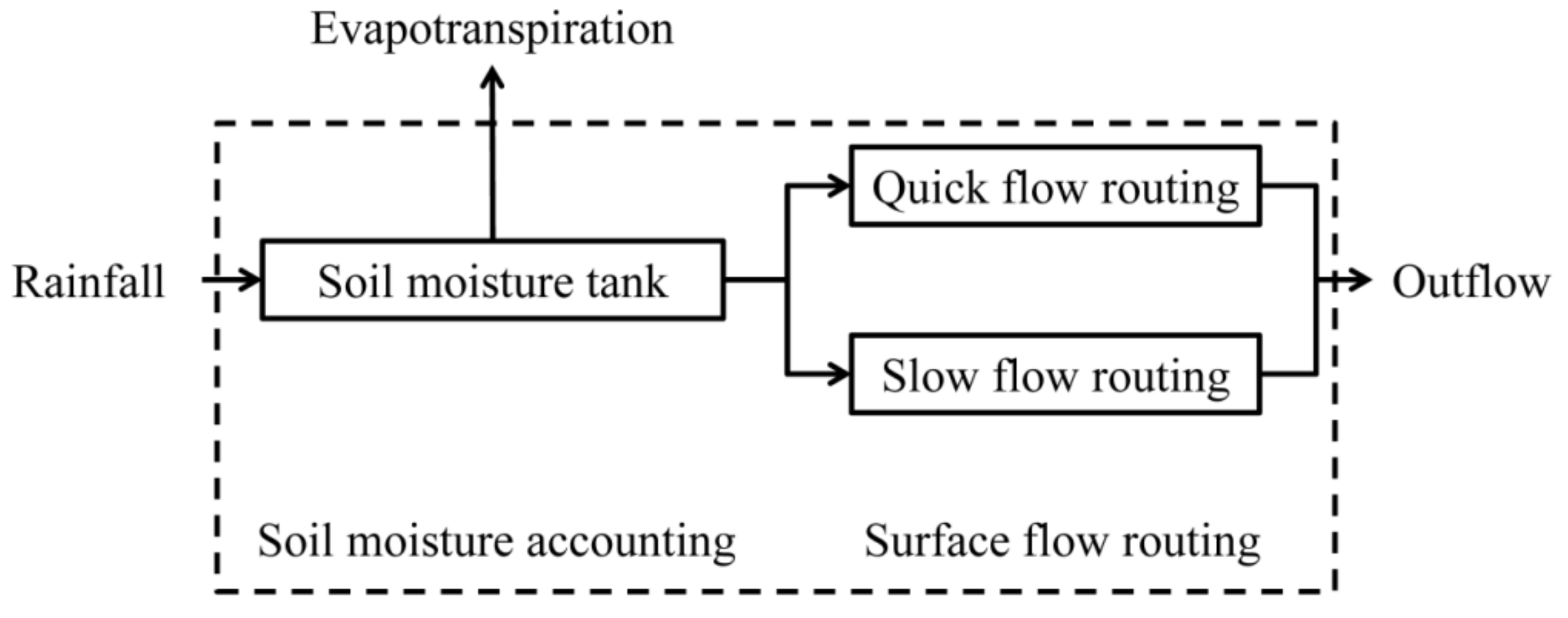
HYMOD is a six-parameter hydrological model running on MATLAB platform (R2015a, MathWorks, Inc., Natick, MA, USA) that simulates the rainfall-runoff process of watersheds [30]. The six parameters include the maximum storage of the soil moisture tank Cpar, the shape parameter b, the ratio of quick flow to total flow α, the number of linear tanks with quick flow Nq, the quick flow coefficient Kq and the slow flow coefficient Ks. HYMOD has a relatively simple model structure, thereby making it suitable for testing the impact of numerical schemes on model output. The configuration of HYMOD is shown in Figure 1. The model contains a soil moisture accounting (SMA) module and a surface flow routing (SUFR) module. A brief description of the mathematical formulations in HYMOD is presented in the following section.
2.2.2. Mathematical Description
SMA converts rainfall excess into the inflow of SUFR. The mass conservation equation for SMA can be expressed as:
where QSMT represents outflow from the soil moisture tank, P represents precipitation, E represents evapotranspiration and C represent the filled storage of the soil moisture tank, which is assumed to be a function of the water depth of the soil moisture tank, H and takes the following form:
where Hpar represents the maximum water depth of the soil moisture tank and b is a shape parameter. H is used as an indicator of the saturation degree of the river basin, which resembles the groundwater level, soil moisture and so forth. A warm-up period can be used in the simulation when no data can be obtained to prescribe an initial condition for H.
SUFR has two components: quick flow routing (QFR) and slow flowing routing (SLFR). QFR can be conceptualized as a Nash cascade process that consists of multiple linear reservoirs with the same outflow coefficient (Kq). The storage equation of the linear reservoir with storage Xq, inflow Iq and outflow Oq can be expressed by:
For a Nash cascade process with n linear reservoirs, the mass conservation can be expressed in a vector form as [31]:
SLFR is similar to QFR except that only one linear reservoir is utilized; therefore, the governing equation of SLFR is similar to Equation (3) and can be expressed as:
where Xs, Is, Os and Ks are the storage, inflow, outflow and outflow coefficient for the linear reservoir in SLFR. An additional parameter, α, is introduced to determine the fractions of QSMT that flow to QFR and SLFR using the following equation:
Equations (1), (2) and (4)–(6) form the governing equation set for HYMOD.
2.2.3. Analytical Solution to SMA
No numerical solutions are necessary in solving the governing equation for SMA (Equation (1)) because the outflow depends only on the initial and final state of the basin storage (P and E are user-prescribed parameters). In deriving an analytical solution to SMA, an additional equation is required to close the governing equation. Moore [30] assumed the depth of soil moisture tank was increased by rainfall, was depleted by evapotranspiration and generation of direct runoff occurred when rainfall exceeded the storage capacity. Therefore, the following relationship is assumed:
Equation (7) indicates that all rainfall excess infiltrates into the soil moisture tank and water depth in the tank rises correspondingly. By taking the derivatives with respect to H on both sides of Equation (2), we obtain:
By substituting Equations (7) and (8) into Equation (1), we obtain the analytical form of QSMT:
Equation (9) is the analytical form for QSMT in this study. It should be noted that Equation (9) is valid only when H < Hpar. Once H exceeds Hpar, infiltration no longer occurs and all rainfall excess is converted into surface runoff.
2.2.4. Numerical Schemes
In this section, we formulate the numerical schemes for discretizing the storage equations of the linear reservoirs in both QFR and SLFR. The storage equation of a linear reservoir can be expressed as:
By integrating on both sides of the storage equation from time t to t + Δt, we obtain:
For the ith reservoir in a Nash cascade process, Equation (10) can be written as:
The integral of X(t) from t to t + Δt needs to be evaluated with numerical schemes. The explicit Runge-Kutta schemes and the partially implicit Euler schemes are briefly introduced in the following sections.
2.2.4.1. The Explicit Runge-Kutta Schemes
The explicit Runge-Kutta schemes are a class of numerical schemes with zero implicit factor and variable orders of accuracy. In this study, the first- to fourth-order explicit Runge-Kutta schemes are introduced to evaluate the integral of X(t), which can be expressed as follows.
The first-order explicit Runge-Kutta scheme (RK1):
The second-order explicit Runge-Kutta scheme (RK2):
The third-order explicit Runge-Kutta scheme (RK3):
The fourth-order explicit Runge-Kutta scheme (RK4):
where O(p) represents the truncation error terms, which is order p, resulted from using the numerical schemes to approximate the integrals. According to Equation (3), the derivative can be evaluated by:
2.2.4.2. The Partially-Implicit Euler Schemes
A generalized form of the partially-implicit Euler schemes can be expressed as:
where θ represents the implicit factor ranging from 0 to 1. Equation (18) indicates that the partially-implicit Euler schemes evaluate the temporal integration time t to t + Δt as a weighted average of the integrals at the previous (t) and the current (t + Δt) time steps. When θ = 0, the scheme is called the fully explicit Euler scheme (EXP), which has exactly the same form as RK1 (Equation (13)); when θ = 1, the scheme is called the fully implicit Euler scheme (IMP); when 0 < θ < 1, the scheme is called the partially-implicit Euler scheme (PIM). EXP and IMP can also be viewed as two special types of partially-implicit Euler schemes; therefore, we use the term partially-implicit Euler schemes to refer to all three types of numerical schemes in the rest of this study. The partially-implicit Euler schemes generally have first-order accuracy, except for θ = 1/2. The original HYMOD uses EXP by default.
2.2.5. Analytical Solutions to QFR and SLFR
Both QFR and SLFR can be viewed as the Nash cascade process. Szöllösi-Nagy [31] derived an analytical solution for the Nash cascade process, in which the outflow rate of the ith linear reservoir at time t + Δt, Oi(t + Δt), can be expressed in terms of its storage at time t as:
with
where k represents the outflow coefficient and Ii represents the inflow of the ith linear reservoir. In the present study, the analytical solution to HYMOD is obtained from Equations (9) and (19).
2.3. The Downhill Simplex Method (DSM) for Parameter Optimization
The DSM is a nonlinear optimization technique, which was employed in this study to find optimal parameter combinations that correspond to functional minimums. The optimization starts with an initial simplex consisting of m vertices, each of which represents a randomly generated parameter set. The functional minimum in the parameter space can be found by transforming the simplex according to the functional values at the vertexes and moving the simplex in the downhill direction until the functional value converges to its minimum value. Readers may refer to Nelder and Mead [32] for more details about the DSM.
2.4. Model Setup
In this study, we tested the influence of numerical schemes on the output of HYMOD with a series of numerical tests including the simulations of the Nash cascade process, the flow hydrograph of Leaf River basin with a priori parameter set and 2000 random parameter sets, the one-dimensional and two dimensional sensitivity analyses on model parameters and the DSM optimization test.
The Nash cascade process is a basic component of QFR and SLFR. Therefore, we simulated the Nash cascade process to test the influence of numerical schemes on QFR and SLFR. The simulation was carried out with one to ten linear reservoirs in the Nash cascade process. The storage coefficients Kq of the reservoirs were set identical at 0.5. One unit volume of pulsed inflow was given to the first reservoir and the outflow hydrograph of the last reservoir was simulated and compared with the analytical solution (Equations (9) and (19)) to assess the performance of the numerical schemes.
The simulation on Leaf River basin was carried out first with a priori parameter set (Table 1) and then with 2000 randomly generated parameter sets that were generated from a uniform distribution in the parameter space. In the priori parameter set, the flow hydrographs simulated by different numerical schemes were compared with that computed by the analytical solution and the observed data to assess the influence of numerical schemes on model output. In the random parameter test, the mean squared error (MSE) was used as a measure of the overall scheme performance over a wide range of model parameter. The entire 40-year sampling period (1 October 1948 to 30 September 1988) was simulated but only the results from January 1970 to January 1972 were plotted for better visibility.
The response sensitivity of the six model parameters (Cpar, b, α, Nq, Ks and Kq) was assessed by the one-dimensional sensitivity analysis (1DSA) and two-dimensional sensitivity analysis (2DSA). The sensitivity analysis was carried out by varying the values of the parameters being tested within their feasible ranges (Table 1) while holding the other parameters fixed at their priori values.
In the DSM optimization, five model parameters (Cpar, b, α, Ks and Kq) were optimized to find the best combination of model parameters that minimized the MSEs of the computed flow hydrograph. Nq was not utilized in the optimization because it was a discrete variable whose value could not be arbitrarily prescribed. Eight initial parameter sets (Table 2) were used to test the performances of the numerical schemes in different regions of the parameter space. A total of 300 steps were carried out during each DSM optimization.
3. Results
3.1. The HYMOD Simulations for the Leaf River Basin with a Priori Parameter Set
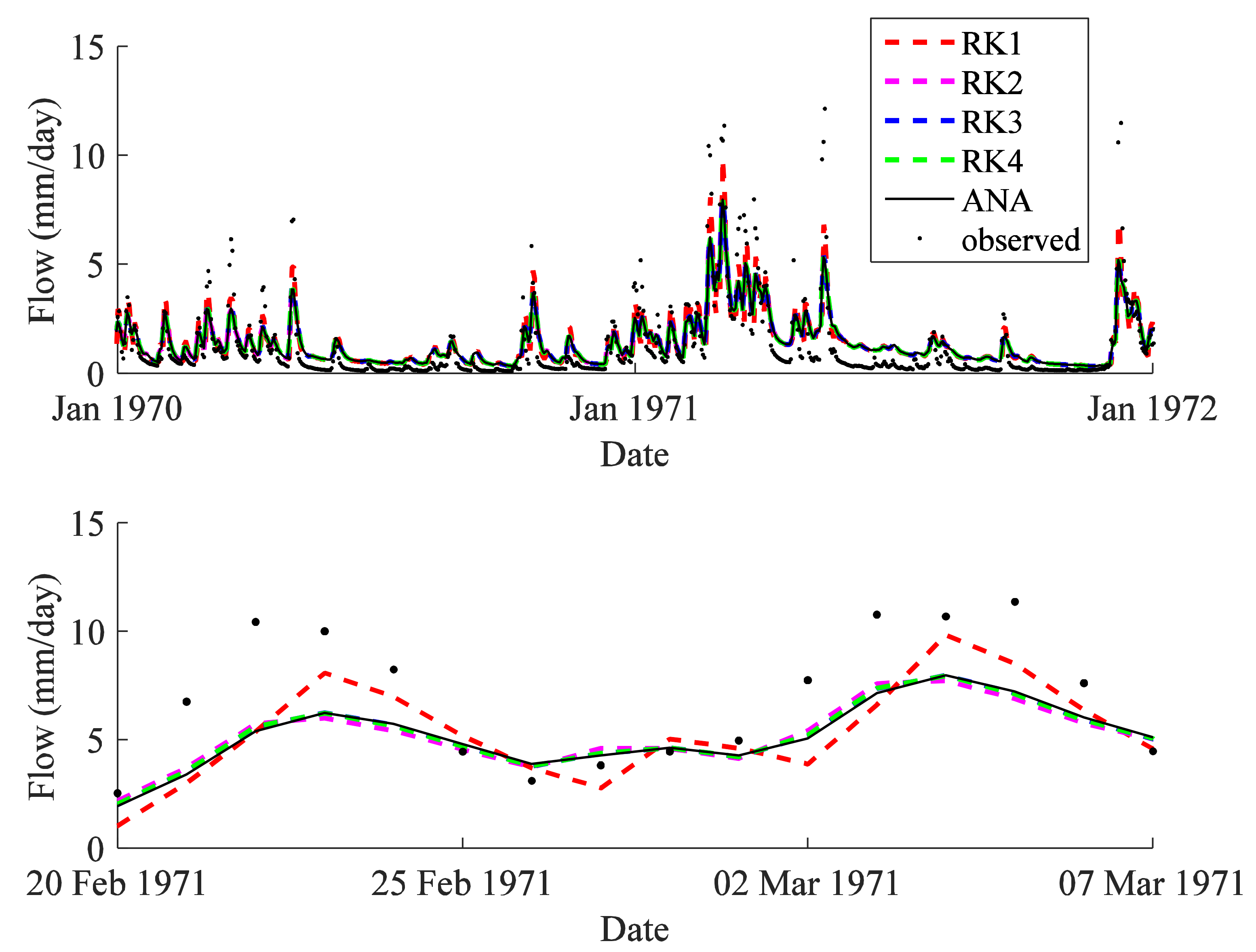
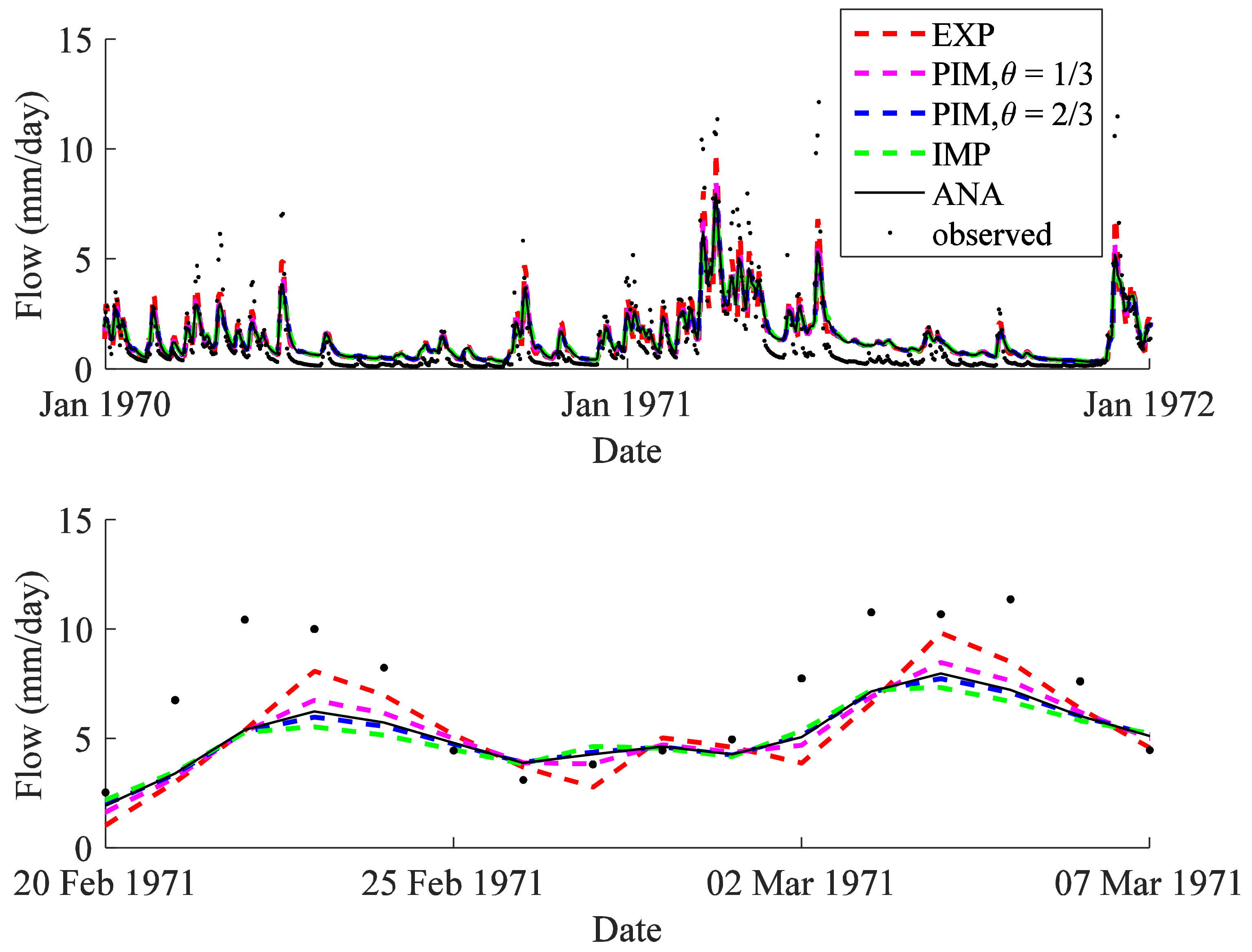
The flow hydrographs of the Leaf River basin simulated with the priori parameter set (Table 1) by the explicit Runge-Kutta schemes (RK1 to RK4) were compared with the analytical solutions (Equations (9) and (19)) and the observed data in Figure 2. The analytical solutions deviated from the observed data likely due to inadequate representation by the priori parameter set. Compared with the analytical solutions, RK1 overestimated the flow in the Leaf River basin during high flow conditions and underestimated the flow during low flow conditions, whereas RK2, RK3 and RK4 all yielded better fits to the analytical solution. This is consistent with the findings in the simulation of the Nash cascade process that the first-order explicit scheme is prone to overestimation whereas second-and-higher-order schemes may effectively reduce the error. Similarly, the solutions by the partially implicit Euler schemes (EXP, PIMs with θ = 1/3 and 2/3 and IMP) were compared with the analytical solutions and observed data in Figure 3. The differences between the numerical and analytical solutions varied with the implicit factor θ. The more explicit schemes with smaller implicit factors tended to generate solutions with greater fluctuations in the hydrograph, characterized by higher peaks and deeper troughs, than the more implicit Euler schemes with larger implicit factors and vice versa. In both Figure 2 and Figure 3, some numerical schemes produced hydrographs that were even more close to the observed data than that simulated by the analytical solution, which indicates an interaction between numerical schemes and model parameters. In summary, results from the simulation of Leaf River basin confirm the strong influence of numerical schemes on the output from HYMOD.
3.2. The HYMOD Simulations with Random Parameter Sets
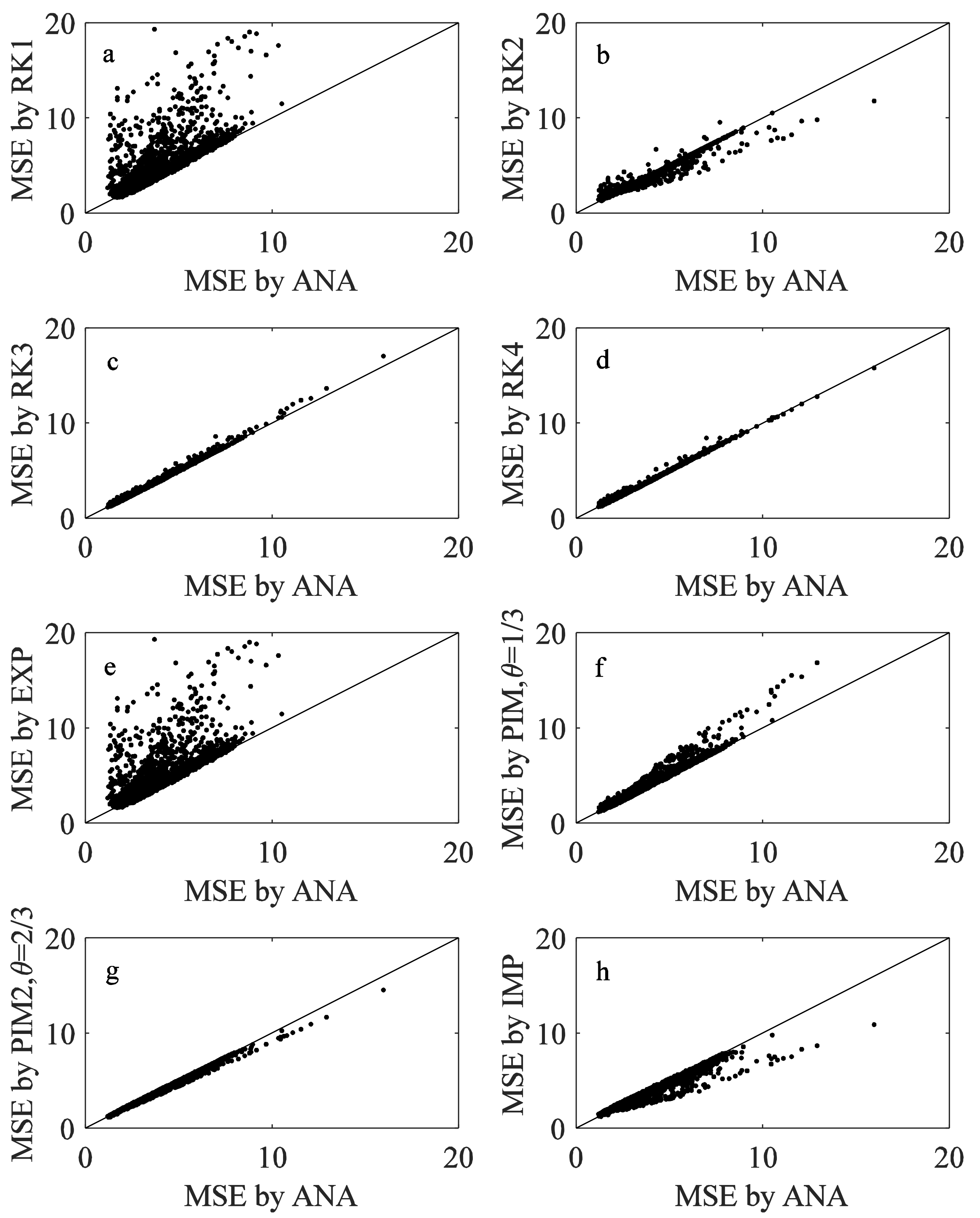
The MSEs of the flow hydrographs simulated by the explicit Runge-Kutta schemes (RK1 to RK4) and the partially implicit Euler schemes (EXP, PIMs with θ = 1/3 and 2/3 and IMP) using the 2000 random parameter sets were compared with those of the analytical solutions in Figure 4. The 1:1 slope in Figure 4 represents the numerical solutions that have equivalent performances as the analytical solutions in terms of MSEs. The numerical solutions computed by RK1 showed a considerable scatter around the 1:1 slope, indicating that RK1 is a poor approximation of the analytical solution over a wide MSE range. In contrast, the numerical solutions computed by RK2 were close to the analytical solution for smaller MSE values but became divergent with increasing MSE values, while RK3 and RK4 provided good approximation to the analytical solution over the whole parameter range, which indicates that high-order explicit Runge-Kutta schemes were more reliable in approximating the analytical solutions than their low-order counterparts. For the partially implicit Euler schemes, the implicit factor seemed to determine whether the MSEs produced by the numerical schemes were larger or smaller than those by the analytical solutions. Results showed that the MSEs showed a tendency to decrease with increasing implicit factor over the entire parameter range: EXP (RK1) and IMP produced larger and smaller MSEs than the analytical solutions, respectively and PIMs with θ = 1/3 and 2/3 produced MSEs that were similar to the analytical solutions. Therefore, the two properties of a numerical scheme, that is, order of accuracy and implicit factor, may influence the simulation results in different ways: the latter may determine the direction in which the numerical solution deviates from the analytical solution, whereas the former may determine how far it deviates.
The lowest MSE computed by a numerical scheme using the 2000 random parameter sets represents the best performance that can be achieved by the scheme and is therefore of particular importance in model calibration. We tabulated the lowest MSEs for all the numerical schemes and the corresponding parameter sets in Table 3. Results showed that the lowest MSEs computed by the schemes were fairly similar except for RK1 and RK2 which produced slightly higher MSEs. Among the schemes, only RK3, RK4 and PIM with θ = 1/3 identified the same parameter set as that found by the analytical solution, whereas the other schemes pointed to different parameter sets. Despite the different parameter sets identified, the PIM with θ = 2/3 and IMP produced similar MSE minima as the analytical solutions, which indicates that model parameters may sometimes compensate for the inadequacy in numerical schemes.
The computational time for 200,000 repeated Nash Cascade simulations with 10 linear reservoirs and 2000 Leaf River basin simulations with random parameter sets was summarized in Table 4 to assess the computational cost of all the numerical schemes. In both cases, the analytical solutions were remarkably computationally more expensive than all the numerical solutions due to its complex form. The computational time for the explicit Runge-Kutta schemes (RK1 to RK4) increased rapidly with the order of accuracy in the scheme because of the increasing number of points at which the integrated function must be evaluated. The partially implicit Euler schemes (PIMs with θ = 1/3 and 2/3 and IMP) were evidently lower than the high-order explicit Runge-Kutta schemes (RK3 and RK4) owing to an optimized algorithm for solving linear equation systems. Therefore, the computational cost of a numerical scheme also varies with its order of accuracy and implicit factor, which should also be considered in selecting numerical schemes for hydrological models.
3.3. Sensitivity Analysis
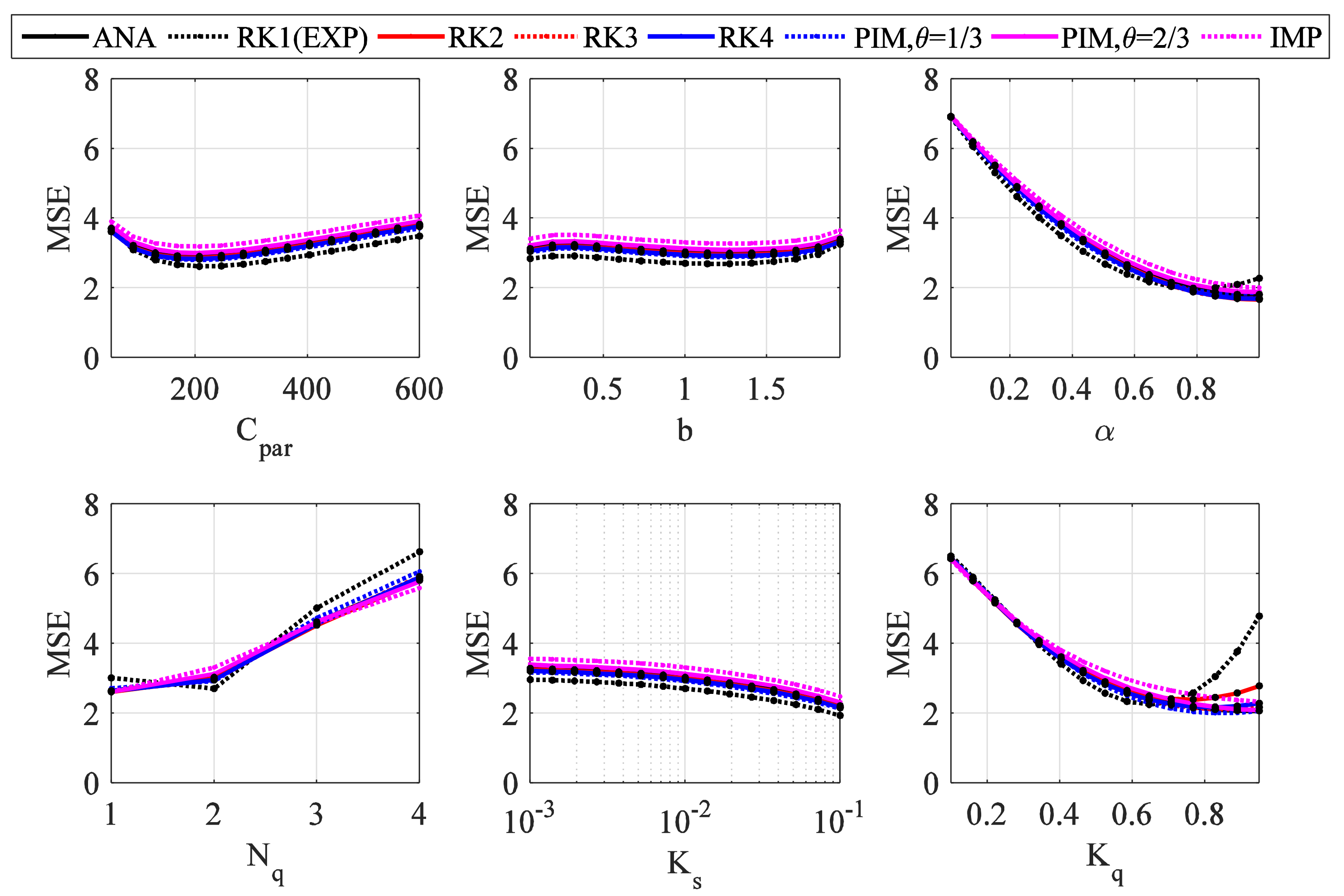
The results of 1DSA were plotted in Figure 5. Results showed that the MSEs of the simulated hydrographs computed by different numerical schemes were sensitive to the variations in α, Nq and Kq but less so to Cpar, b and Ks. Because α, Nq and Kq were all associated with QFR, we may conclude that the parameters in QFR had a stronger impact on the output of HYMOD than those in SMA and SLFR. The MSE curves computed by RK1 (EXP) showed U-shaped distributions for α, Nq and Kq, whereas those computed by other schemes showed monotonic trends with increasing parameter values. For Cpar, b and Ks, the patterns of the MSE curves were relatively similar. Because α, Nq and Kq were all associated with QFR while Cpar, b and Ks were employed by SMT and SLFR, we may conclude that the effect of numerical schemes was more pronounced with the QFR parameters.
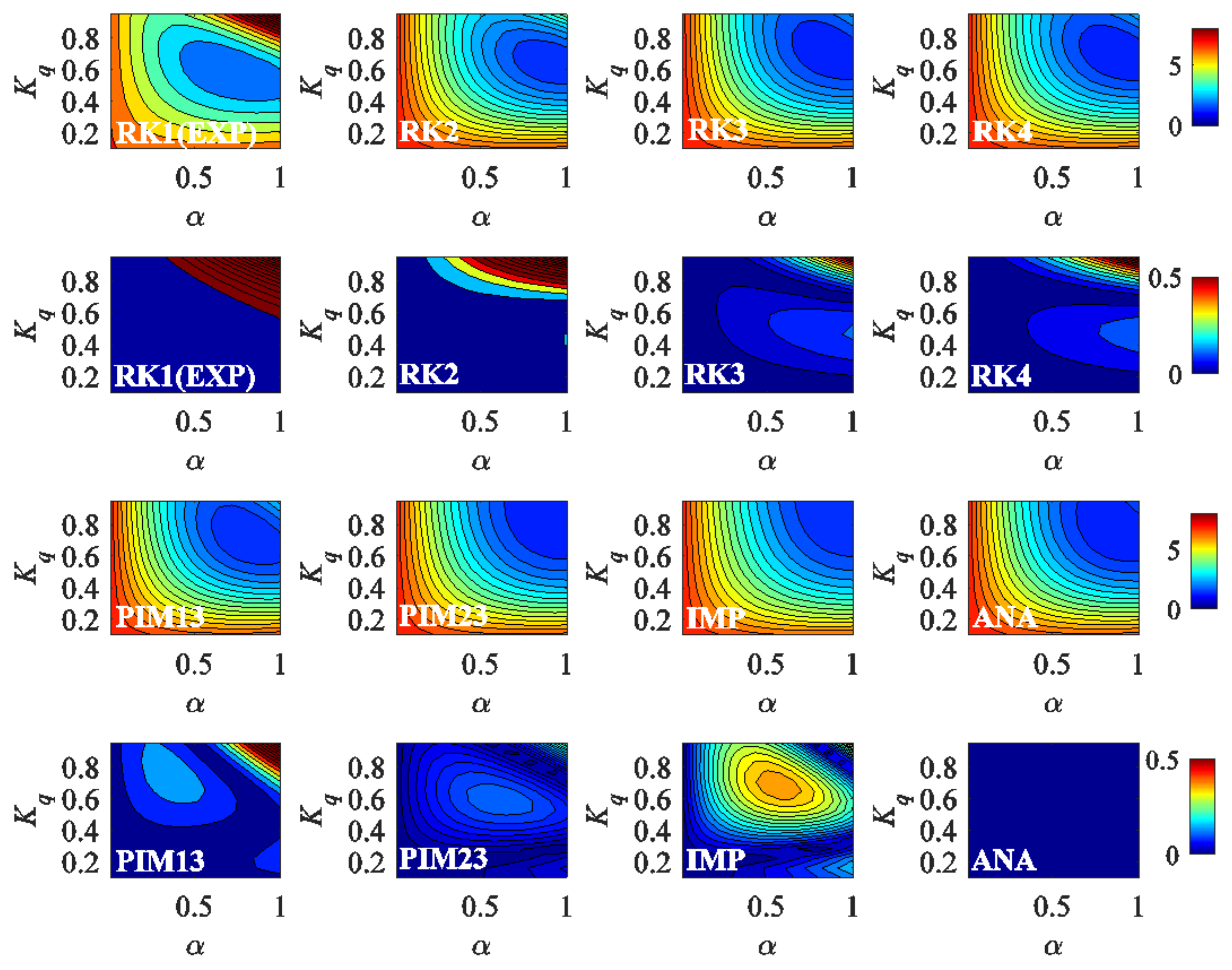
The MSE response surfaces computed in the 2DSA for α and Kq were plotted in Figure 6. The spatial patterns of the MSE response surfaces for different numerical schemes were similar, except for EXP (RK1). A high MSE region was located in the upper-right corner of the MSE response surface computed by EXP (RK1) but not in those computed by other numerical schemes. The high MSE region indicates that the numerical solution of EXP (RK1) significantly deviated from the analytical solution at large Kq and α values due to excessive numerical error, whereas other numerical schemes could approximate the analytical solution over a wider parameter range. The influence of numerical schemes on simulated hydrographs can be seen more clearly in the spatial pattern of MSE difference between the numerical and analytical solutions, which were also plotted in Figure 6. The MSE difference in the upper-right corner of the response surface was effectively reduced by increasing the order of accuracy in the numerical scheme, although this might cause the MSE difference to increase slightly near the right edge of the response surface. The MSE difference could also be reduced by increasing the implicit factor. However, a second zone with significant MSE difference emerged in the central part of the response surface as the implicit factor increased, especially in the case computed by IMP, although this did not necessarily change the pattern of MSE response surface. In summary, low-order explicit schemes may distort the results of sensitivity analysis and this problem can be alleviated but not completely settled by increasing the order of accuracy or adding an implicit factor into the numerical schemes.
3.4. The DSM Optimization
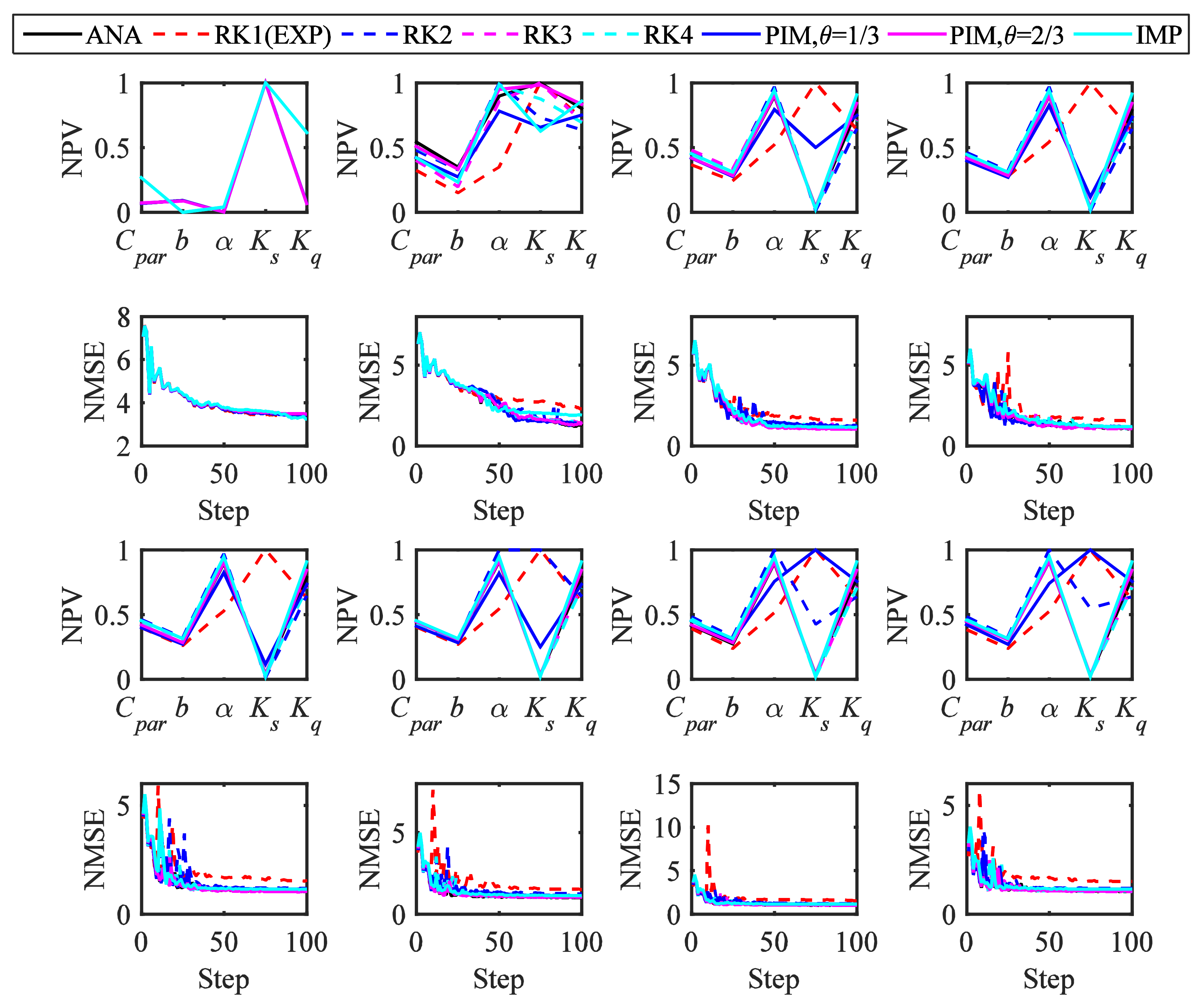
The optimal parameter sets identified by the numerical and analytical solutions and the MSE variation during each optimization are plotted in Figure 7. In all cases, the MSE values were stabilized at the end of the optimization, indicating that the optimization was successfully accomplished. The optimal parameters varied greatly in most cases, confirming the substantial impact of the numerical scheme on parameter optimization. To assess the overall performances of numerical schemes in the DSM optimization, we rated each optimization with regard to three different levels: if the difference between the optimized parameter computed by the numerical solution and the analytical solution was less than 10% of the parameter range, the optimization was classified as good; if the difference was larger than 10% but less than 30% of the parameter range, the optimization was classified as acceptable; otherwise it was classified as poor. The results were tabulated in Table 5 (G, A and P stand for “good,” “acceptable” and “poor”).
As shown in Table 5, the performances of the numerical schemes showed a strong dependence on initial parameter sets. Except for PIM with θ = 2/3 which showed good performances with all the initial parameter sets, all the numerical schemes provided acceptable or poor performances in some of the test cases. Both the order of accuracy and implicit factor were shown to influence the effectiveness of the DSM optimization. For the explicit Runge-Kutta schemes (RK1 to RK4), the scheme performance generally improved with increasing order of accuracy: RK1 identified the optimal parameter set in only one of the test cases, whereas RK2 to RK4 were successfully applied in a wider parameter range. For the partially implicit Euler schemes (EXP, PIMs with θ = 1/3 and 2/3 and IMP), the scheme performance first improved and then deteriorated with increasing implicit factor. PIM with θ = 2/3 provided the best overall performance among all the numerical schemes, which also demonstrates that the scheme performance did not vary monotonically with increasing implicit factor. In the optimization process, the MSEs for different numerical schemes converged at a similar speed, indicating that the schemes did not significantly affect the convergence rate of the optimization process. Except for EXP (RK1), all numerical schemes reached a similar MSE level at the end of the optimization, which illustrates how the model parameters compensated for the numerical error and affected the results of the DSM optimization.
4. Discussion
4.1. Source of Numerical Error in HYMOD Simulations
Results of this study reveal a strong dependence of model output on numerical schemes. In the simulation of the Leaf River basin, both the order of accuracy and the implicit factor significantly affected the simulated flow hydrograph but in different ways: the implicit factor determined whether the flow hydrograph was overestimated or underestimated, whereas the difference between the numerical and analytical solutions decreased with increasing orders of accuracy.
The scheme dependence of the numerical results indicates the existence of numerical error, which is originated from the truncation error when using a numerical scheme to approximate the analytical solution to the storage equation of the linear reservoirs. Since the order of accuracy is a measure of the magnitude of truncation error pertaining to a numerical scheme, it is immediately seen that RK1 to RK4 were characterized by truncation errors of O(Δt2) to O(Δt5). Therefore, the numerical error in the flow hydrograph simulated by high-order Runge-Kutta schemes was smaller than that by low-order Runge-Kutta schemes. For partially implicit Euler schemes (Equation (18)), the truncation error can be expressed as:
Equation (23) shows that the leading error term can change sign as the implicit factor, θ, in the partially implicit Euler schemes varies between 0 and 1, which causes the flow hydrograph to be overestimated and underestimated.
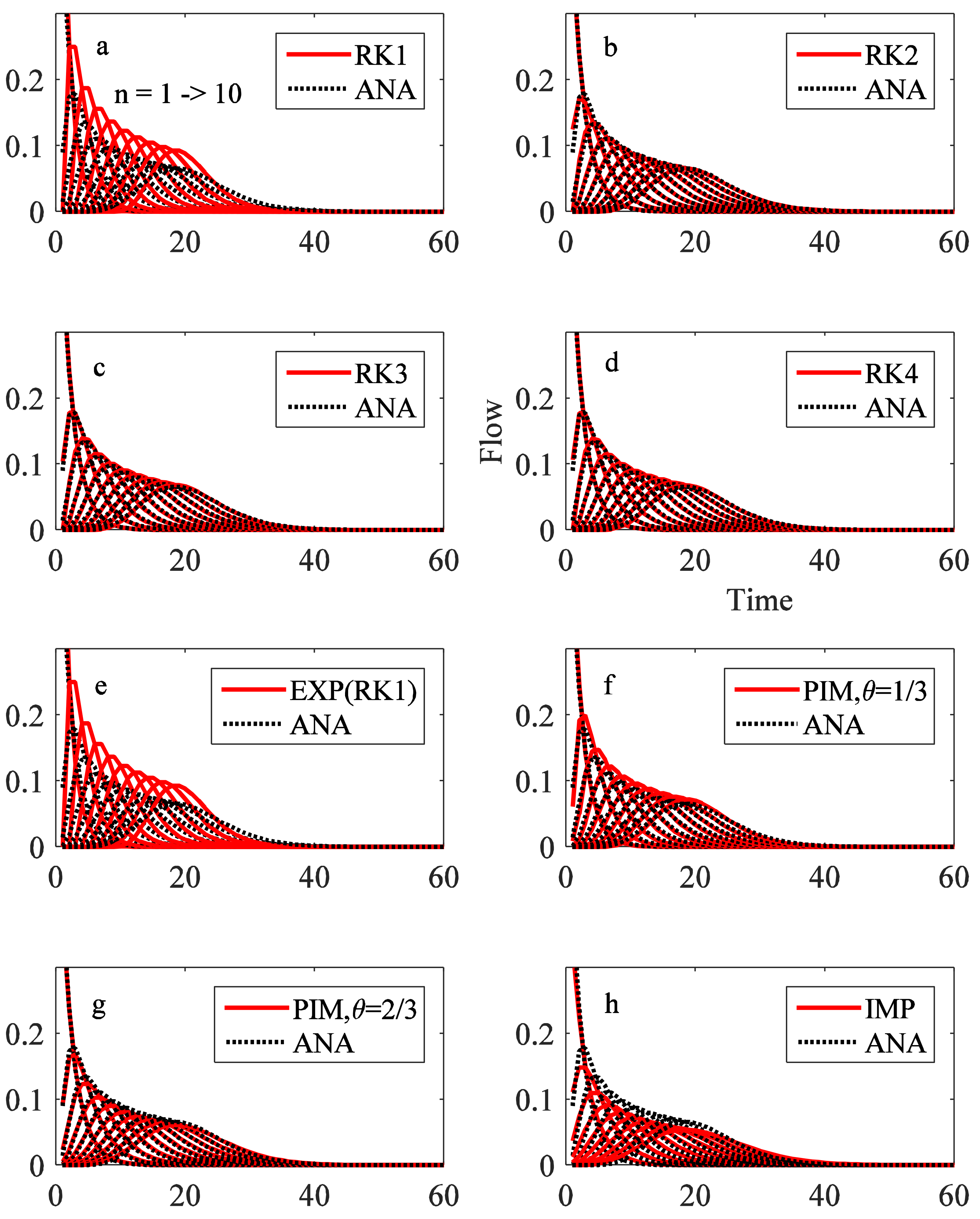
The Nash cascade process can be used to demonstrate how numerical error varies with numerical schemes. The outflow hydrographs with one to ten linear reservoirs were simulated by the explicit Runge-Kutta schemes (RK1 to RK4) and the partially implicit Euler schemes (EXP, PIMs with θ = 1/3 and 2/3 and IMP) and compared with the analytical solutions computed by Equations (9) and (19). Results (Figure 8) showed that the difference between the numerical and analytical solutions decreases with increasing order of accuracy and first decreases and then increases with increasing implicit factor. This is consistent with the simulation results of the Leaf River basin presented in Figure 2 and Figure 3, which confirms that the source of numerical error in HYMOD simulations is the truncation error of the numerical schemes that were used in simulating the Nash cascade process. Since both QFR and SLFR are conceptualized as Nash cascade processes which differed only in the number of linear reservoirs being employed, numerical schemes may impose their impacts on both of these components.
4.2. Implications for Hydrological Modeling
In previous studies, modelers commonly apply an ad-hoc numerical scheme without considering the adequacy of the numerical scheme. Our results demonstrate the need for implementing suitable numerical schemes in hydrological models. In the simulation of the Leaf River basin, different numerical schemes induced a scheme-dependent bias in the predictions of flow hydrograph (Figure 4). In addition, excessive numerical error induced by unsuitable numerical schemes may also distort the response sensitivity surfaces and bring unnecessary challenges to the gradient-based optimization methods. In 1DSA (Figure 5), the numerical schemes changed the monotonicity of the MSE curves for α and Kq. In 2DSA (Figure 6), RK1 (EXP) produced a false high-MSE region in the α-Kq response sensitivity surface. Kavetski and Clark [28] presented a case in which the response sensitivity surface was so strongly distorted that the optimal region could not be clearly defined. Therefore, the adequacy of the numerical schemes in hydrological models should be carefully considered.
Model parameters may sometimes compensate for the inadequacy in numerical schemes owing to the interaction between them. The simulation results with random parameter sets (Table 3) showed that all of the tested schemes, except RK1 (EXP) and RK2, generated similar flow hydrographs using different parameter sets. In other words, it is possible to obtain similar predictions using poor numerical schemes as those with “good” numerical schemes by tuning model parameters. However, this characteristic is not favorable in model development because structural identifiability is compromised by inappropriate implementation of numerical schemes. For example, the DSM optimization with IMP only provided acceptable or poor performances in all the test cases, which indicates that the best parameter sets identified by IMP is notably different from those identified by the analytical solutions. This will cause discrepancy in optimized model parameters and consequently the model predictions if we do not explicitly report the numerical schemes being used in the study.
The performance of a numerical scheme is closely associated with its numerical error, which should be controlled in obtaining the numerical solutions. The form of Equation (19) suggested that there are two possible solutions to reduce the truncation error of numerical schemes. The first solution is to reduce the size of the time step in the model simulation. However, this is not always feasible in hydrological studies, because the time step in performing a hydrological simulation needs to be compatible with the resolution of the input data. In this study, a daily time step is a natural choice because daily precipitation and evapotranspiration is provided as model input. To adopt a small time step in the simulation, the input data needs to be downscaled with interpolation techniques, which will bring additional source of error into the model output.
The other solution is to choose an appropriate numerical scheme for the hydrological model that faithfully reflects the property of the analytical solutions. However, it is impossible to test the performances of all the numerical schemes for hydrological model studies. Besides, the analytical solution is usually not available for most advanced hydrological models. To seek a suitable numerical scheme without assessing all possible candidates, one needs to understand the relationship between model performance and the common properties of numerical schemes, such as the order of accuracy and the implicit factor. Our results suggested that the use of lower-order explicit schemes should be avoided in modeling practice. This is consistent with the conclusions drawn by Clark and Kavetski [25], who disapproved the use of a fixed-step first-order explicit scheme. Clark and Kavetski [25] also recommended the use of IMP in parameter optimization, which produced smooth response surfaces in their sensitivity analysis. However, IMP did not identify the optimal parameter sets in two of the eight test cases in our study, suggesting that the low-order implicit schemes should also be used with caution in hydrological models. On the other hand, high order explicit Runge-Kutta schemes, such as RK3 and RK4, require higher computational cost than the partially implicit Euler schemes in computing the integral terms in simulating the Nash cascade process. Therefore, the partially implicit Euler schemes with the implicit factor ranging between 1/3 and 2/3 were recommended based on the HYMOD simulations presented in this study.
5. Conclusions
The importance of numerical schemes in hydrological models has not been well recognized in previous hydrological studies. In this study, we evaluated the effect of numerical schemes on hydrological simulations. HYMOD was employed with two types of numerical schemes (i.e., the explicit Runge-Kutta schemes and the partially implicit Euler schemes) to simulate the flow hydrograph of the Leaf River basin from 1948 to 1988. We did not limit ourselves to the comparison between specific numerical schemes but rather focused on finding a generalized relationship between model performance and the two common properties of numerical schemes (i.e., the order of accuracy and the implicit factor). The effects of the order of accuracy and the implicit factor on the model simulation, sensitivity analysis and parameter optimization were discussed. The following conclusions were drawn:
- (1)
- The results of the HYMOD simulations showed a strong dependence on numerical schemes. Both the order of accuracy and the implicit factor significantly affected the simulated flow hydrograph but in different ways: the implicit factor determined whether the flow hydrograph was overestimated or underestimated, whereas the difference between the numerical and analytical solutions decreased with increasing orders of accuracy. The numerical error in the simulation is originated from the truncation error when using a numerical scheme to discretize the storage equation of the linear reservoirs. For the explicit Runge-Kutta schemes, the magnitude of numerical error decreases with increasing order of accuracy and thus the high-order Runge-Kutta schemes produced better prediction than the low-order Runge-Kutta schemes did. For the partially implicit Euler schemes, the leading error term may change sign as the implicit factor varies, which causes the flow hydrograph to be overestimated and underestimated.
- (2)
- Numerical error induced by unsuitable numerical schemes may distort the response sensitivity surfaces of hydrological models and cause discrepancy in optimized model parameters. Owing to the interaction between numerical schemes and model parameters, model parameters may sometimes compensate for the inadequacy in numerical schemes. However, this is not favorable in model development because the model structural identifiability is compromised by inappropriate implementation of numerical schemes. Therefore, the adequacy of the numerical schemes in hydrological models should be carefully considered.
- (3)
- Results of the numerical tests have important implications for selecting suitable numerical schemes for hydrological models. The performance of a numerical scheme is closely associated with its numerical error, which can be controlled either by reducing the time step or by choosing a numerical scheme that well approximates the analytical solutions. However, reducing the time step is not always feasible in hydrological studies due to issues in data availability. To design a new scheme for a hydrological model without assessing all possible candidates, one needs to understand the link between model performance and the common properties of numerical schemes, such as the order of accuracy and the implicit factor. The use of lower-order explicit schemes should be avoided and the low-order implicit schemes should also be used with caution in hydrological modeling studies. On the other hand, high order explicit Runge-Kutta schemes require higher computational cost than the partially implicit Euler schemes. Based on the HYMOD simulations presented in this study, we recommended the use of partially implicit Euler schemes with the implicit factor ranging between 1/3 and 2/3. This study demonstrates that the uncertainty in the output of hydrological models can be effectively reduced by choosing numerical schemes with proper orders of accuracy and implicit factors, which provides an optimized balance between model performance and computational cost.
Author Contributions
S.Z. and K.A-A. conceived the study; S.Z. performed the numerical analysis and wrote the paper; K.A-A. revised the paper.
Funding
This research was funded by National Key R&D Program of China, grant number 2016YFC0402406 and National Natural Science Foundation of China, grant number 51509234, 51579230.
Acknowledgments
The authors gratefully thank Professor Hoshin V. Gupta for providing the HYMOD program and hydrological data and Dr. Yang Bai for her contribution in an early stage of the project.
Conflicts of Interest
The authors declare no conflict of interest. The funders had no role in the design of the study; in the collection, analyses or interpretation of data; in the writing of the manuscript or in the decision to publish the results.
References
- Arnold, J.G.; Srinivasan, R.; Muttiah, R.S.; Williams, J.R. Large area hydrologic modeling and assessment Part I: Model development. J. Am. Water Resour. Assoc. 1998, 34, 73–89. [Google Scholar] [CrossRef]
- Beven, K.J.; Kirkby, M.J. A physically based, variable contributing area model of basin hydrology. Hydrol. Sci. J. 1979, 24, 43–69. [Google Scholar] [CrossRef]
- Bergström, S.; Forsman, A. Development of a conceptual deterministic rainfall–runoff model. Nord. Hydrol. 1973, 4, 147–170. [Google Scholar] [CrossRef]
- Lindström, G.; Pers, C.; Rosberg, J.; Strömqvist, J.; Arheimer, B. Development and test of the HYPE (Hydrological Predictions for the Environment) model – a water quality model for different spatial scales. Hydrol. Res. 2010, 41, 295–319. [Google Scholar] [CrossRef]
- Kitanidis, P.K.; Bras, R.L. Real-Time Forecasting with a Conceptual Hydrologic Model 1. Analysis of Uncertainty. Water Resour. Res. 1980, 16, 1025–1033. [Google Scholar] [CrossRef]
- Kitanidis, P.K.; Bras, R.L. Real-Time Forecasting with a Conceptual Hydrologic Model 2. Applications and Results. Water Resour. Res. 1980, 16, 1034–1044. [Google Scholar] [CrossRef]
- Liang, X.; Lettenmaier, D.P.; Wood, E.F.; Burges, S.J. A Simple Hydrologically Based Model of Land-Surface Water and Energy Fluxes for General-Circulation Models. J. Geophys. Res.-Atmos. 1994, 99, 14415–14428. [Google Scholar] [CrossRef]
- Srinivasan, R.; Ramanarayanan, T.S.; Arnold, J.G.; Bednarz, S.T. Large area hydrologic modeling and assessment - Part II: Model application. J. Am. Water Resour. Assoc. 1998, 34, 91–101. [Google Scholar] [CrossRef]
- Tang, Q.; Oki, T.; Kanae, S.; Hu, H. The influence of precipitation variability and partial irrigation within grid cells on a hydrological simulation. J. Hydrometeorol. 2007, 8, 499–512. [Google Scholar] [CrossRef]
- Samaniego, L.; Kumar, R.; Attinger, S. Multiscale parameter regionalization of a grid---based hydrologic model at the mesoscale. Water Resour. Res. 2010, 46, W05523. [Google Scholar] [CrossRef]
- Best, M.J.; Pryor, M.; Clark, D.B.; Rooney, G.G.; Essery, R.L.H.; Ménard, C.B.; Edwards, J.M.; Hendry, M.A.; Porson, A.; Gedney, N.; et al. The Joint UK Land Environment Simulator (JULES), model description - Part 1: Energy and water fluxes. Geosci. Model. Dev. 2011, 4, 677–699. [Google Scholar] [CrossRef]
- Krysanova, V.; Hattermann, F.; Wechsung, F. Development of the ecohydrological model SWIM for regional impact studies and vulnerability assessment. Hydrol. Processes 2005, 19, 763–783. [Google Scholar] [CrossRef]
- Fenicia, F.; Kavetski, D.; Savenije, H.H.G. Elements of a flexible approach for conceptual hydrological modeling: 1. Motivation and theoretical development. Water Resour. Res. 2011, 47, W11510. [Google Scholar] [CrossRef]
- Kavetski, D.; Fenicia, F. Elements of a flexible approach for conceptual hydrological modeling: 2. Application and experimental insights. Water Resour. Res. 2011, 47, W11511. [Google Scholar] [CrossRef]
- Beck, H.E.; van Dijk, A.I.J.M.; de Roo, A.; Dutra, E.; Fink, G.; Orth, R.; Schellekens, J. Global evaluation of runoff from 10 state-of-the-art hydrological models. Hydrol. Earth Syst. Sci. 2017, 21, 2881–2903. [Google Scholar] [CrossRef]
- Hattermann, F.F.; Krysanova, V.; Gosling, S.N.; Dankers, R.; Daggupati, P.; Donnelly, C.; Flörke, M.; Huang, S.; Motovilov, Y.; Buda, S.; et al. Cross---scale intercomparison of climate change impacts simulated by regional and global hydrological models in eleven large river basins. Clim. Change 2017, 141, 561–576. [Google Scholar] [CrossRef]
- Wagener, T.; Boyle, D.P.; Lees, M.J.H.; Wheater, S.; Gupta, H.V.; Sorooshian, S. A framework for development and application of hydrological models. Hydrol. Earth Syst. Sci. 2001, 5, 13–26. [Google Scholar] [CrossRef]
- Kirchner, J.W. Getting the right answers for the right reasons: Linking measurements, analyses, and models to advance the science of hydrology. Water Resour. Res. 2006, 42, W03S04. [Google Scholar] [CrossRef]
- Gupta, H.V.; Clark, M.P.; Vrugt, J.A.; Abramowitz, G.; Ye, M. Towards a comprehensive assessment of model structural adequacy. Water Resour. Res. 2012, 48, W08301. [Google Scholar] [CrossRef]
- Clark, M.P.; Nijssen, B.; Lundquist, J.D.; Kavetski, D.; Rupp, D.E.; Woods, R.A.; Freer, J.E.; Gutmann, E.D.; Wood, A.W.; Brekke, L.D.; et al. A unified approach for process-based hydrologic modeling: 1. Modeling concept. Water Resour. Res. 2015, 51, 2498–2514. [Google Scholar] [CrossRef]
- LeVeque, R.J. Finite Volume Methods for Hyperbolic Problems, 1st ed.; Cambridge University Press: Cambridge, UK, 2002; pp. 64–86. [Google Scholar]
- Wu, W. Computational River Dynamics, 1st ed.; Taylor & Francis: New York, NY, USA, 2007; pp. 113–174. [Google Scholar]
- ASME V&V 20 committee. Standard for Verification and Validation in Computational Fluid Dynamics and Heat Transfer; American Society of Mechanical Engineers: New York, NY, USA, 2009. [Google Scholar]
- Gorgoglione, A.; Bombardelli, F.A.; Pitton, B.J.L.; Oki, L.R.; Haver, D.L.; Young, T.M. Uncertainty in the parameterization of sediment build-up and wash-off processes in the simulation of sediment transport in urban areas. Environ. Model. Softw. 2019, 111, pp–170. [Google Scholar] [CrossRef]
- Clark, M.P.; Kavetski, D. Ancient numerical daemons of conceptual hydrological modeling: 1. Fidelity and efficiency of time stepping schemes. Water Resour. Res. 2010, 46, W10510. [Google Scholar] [CrossRef]
- Clark, M.P.; Slater, A.G.; Rupp, D.E.; Woods, R.A.; Vrugt, J.A.; Gupta, H.V.; Wagener, T.; Hay, L.E. Framework for Understanding Structural Errors (FUSE): A modular framework to diagnose differences between hydrological models. Water Resour. Res. 2008, 44, W00B02. [Google Scholar] [CrossRef]
- Mendoza, P.A.; Clark, M.P.; Mizukami, N.; Gutmann, E.D.; Arnold, J.R.; Brekke, L.D.; Rajagopalan, B. How do hydrologic modeling decisions affect the portrayal of climate change impacts? Hydrol. Processes 2016, 30, 1071–1095. [Google Scholar] [CrossRef]
- Kavetski, D.; Clark, M.P. Ancient numerical daemons of conceptual hydrological modeling: 2. Impact of time stepping schemes on model analysis and prediction. Water Resour. Res. 2010, 46, W10511. [Google Scholar] [CrossRef]
- Schoups, G.; Vrugt, J.A.; Fenicia, F.; de Giesen, N.C.V. Corruption of accuracy and efficiency of Markov chain Monte Carlo simulation by inaccurate numerical implementation of conceptual hydrologic models. Water Resour. Res. 2010, 46, W10530. [Google Scholar] [CrossRef]
- Moore, R.J. The probability-distributed principle and runoff production at point and basin scales. Hydrol. Sci. J. 1985, 30, 273–297. [Google Scholar]
- Szöllösi-Nagy, A. The discretization of the continuous linear cascade by means of state space analysis. J. Hydrol. 1982, 58, 223–236. [Google Scholar] [CrossRef]
- Nelder, J.A.; Mead, R. A Simplex-Method for Function Minimization. Comput. J. 1965, 7, 308–313. [Google Scholar] [CrossRef]
Figure 1.
Configuration of HYMOD.

Figure 2.
Flow hydrographs simulated with analytical solutions and the explicit Runge-Kutta schemes for: January 1970–January 1972 (top) and 20 February 1971–7 March 1971 (bottom).
Figure 2.
Flow hydrographs simulated with analytical solutions and the explicit Runge-Kutta schemes for: January 1970–January 1972 (top) and 20 February 1971–7 March 1971 (bottom).

Figure 3.
Flow hydrographs simulated with analytical solutions and the partially implicit Euler schemes for: January 1970–January 1972 (top) and 20 February 1971–7 March 1971 (bottom).
Figure 3.
Flow hydrographs simulated with analytical solutions and the partially implicit Euler schemes for: January 1970–January 1972 (top) and 20 February 1971–7 March 1971 (bottom).

Figure 4.
Comparison of the mean square error (MSE) computed by the analytical solutions and those by the (a) 1st order Runge-Kutta scheme (RK1); (b) 2nd order Runge-Kutta scheme (RK2); (c) 3rd order Runge-Kutta scheme (RK3); (d) 4th order Runge-Kutta scheme (RK4); (e) explicit Euler scheme (EXP, equivalent to RK1); (f) partially implicit Euler scheme (PIM, θ = 1/3); (g) partially implicit Euler scheme (PIM, θ = 2/3); and (h) implicit Euler scheme (IMP, θ = 1). ANA represents the analytical solution and θ represents the implicit factor.

Figure 5.
One-dimensional sensitivity analysis (1DSA) of the mean square error (MSE) with different numerical schemes for the six parameters in HYMOD.
Figure 5.
One-dimensional sensitivity analysis (1DSA) of the mean square error (MSE) with different numerical schemes for the six parameters in HYMOD.

Figure 6.
Two-dimensional sensitivity analysis (2DSA) with different numerical schemes for α and Kq. First row: mean square error (MSE) response surfaces for RK1 to RK4; second row: MSE difference between the analytical and numerical solutions for RK1 to RK4; third row: MSE response surfaces for the Euler schemes; fourth row: MSE difference between the analytical and numerical solutions for the Euler schemes.

Figure 7.
The optimal parameter values and the variations of the mean square error (MSE) values computed by the eight numerical schemes. First row: Normalized optimal parameter values (NPV) for RK1 to RK4; second row: normalized MSE (NMSE) variations for RK1 to RK4; third row: NPV for the Euler schemes; fourth row: normalized MSE (NMSE) variations for the Euler schemes.

Figure 8.
Comparison between the analytical and numerical solutions with: (a) 1st order Runge-Kutta scheme (RK1); (b) 2nd order Runge-Kutta scheme (RK2); (c) 3rd order Runge-Kutta scheme (RK3); (d) 4th order Runge-Kutta scheme (RK4); (e) explicit Euler scheme (EXP, equivalent to RK1); (f) partially implicit Euler scheme (PIM, θ = 1/3); (g) partially implicit Euler scheme (PIM, θ = 2/3); and (h) implicit Euler scheme (IMP, θ = 1). ANA represents the analytical solution, θ represents the implicit factor and n is the number of linear reservoirs in the Nash cascade process. Curves from left to right in each plot correspond to n increasing from one to ten.


Table 1.
A priori parameter set and feasible parameter ranges.
| Parameter | Cpar | b | α | Nq | Ks | Kq |
|---|---|---|---|---|---|---|
| Priori value | 300 | 1 | 0.5 | 2 | 0.01 | 0.5 |
| Range | 50–600 | 0.05–1.95 | 0.01–1.00 | 1, 2, 3, 4 | 0.001–0.1 | 0.1–0.95 |
Table 2.
Initial parameter sets used in the DSM optimization.
| Set | Cpar | b | α | Nq | Ks | Kq |
|---|---|---|---|---|---|---|
| 1 | 200 | 0.2 | 0.1 | 2 | 0.01 | 0.2 |
| 2 | 250 | 0.4 | 0.2 | 2 | 0.02 | 0.3 |
| 3 | 300 | 0.6 | 0.3 | 2 | 0.03 | 0.4 |
| 4 | 350 | 0.8 | 0.4 | 2 | 0.04 | 0.5 |
| 5 | 400 | 1 | 0.5 | 2 | 0.05 | 0.6 |
| 6 | 450 | 1.2 | 0.6 | 2 | 0.06 | 0.7 |
| 7 | 500 | 1.4 | 0.7 | 2 | 0.07 | 0.8 |
| 8 | 550 | 1.6 | 0.8 | 2 | 0.08 | 0.9 |
Table 3.
The lowest MSEs for the numerical schemes and their corresponding parameter sets.
| Scheme | MSEmin | Cpar | b | α | Nq | Kq | Ks | Same Parameter set as ANA? |
|---|---|---|---|---|---|---|---|---|
| ANA | 1.18 | 318.07 | 0.58 | 0.80 | 2 | 0.02 | 0.020 | - |
| RK1(EXP) | 1.64 | 238.19 | 0.48 | 0.85 | 1 | 0.09 | 0.088 | No |
| RK2 | 1.64 | 238.19 | 0.48 | 0.85 | 1 | 0.09 | 0.088 | No |
| RK3 | 1.16 | 318.07 | 0.58 | 0.80 | 2 | 0.02 | 0.020 | Yes |
| RK4 | 1.20 | 318.07 | 0.58 | 0.80 | 2 | 0.02 | 0.020 | Yes |
| PIM131 | 1.20 | 318.07 | 0.58 | 0.80 | 2 | 0.02 | 0.020 | Yes |
| PIM231 | 1.16 | 284.67 | 0.30 | 0.85 | 2 | 0.00 | 0.002 | No |
| IMP | 1.24 | 306.51 | 0.38 | 0.95 | 2 | 0.01 | 0.010 | No |
Note: 1 PIM13 and PIM23 represent the partially implicit Euler schemes with θ = 1/3 and 2/3, respectively.
Table 4.
Computational time in the random test for all the numerical schemes.
| Scheme | Time (seconds) 1 | |
|---|---|---|
| Nash Cascade simulation (200,000 times) | Random simulation (2000 random sets) | |
| ANA | 3960.6 | 3407.9 |
| RK1 | 227.1 | 2748.7 |
| RK2 | 244.3 | 2992.9 |
| RK3 | 265.7 | 3023.5 |
| RK4 | 268.0 | 3051.6 |
| PIM13 2 | 247.6 | 2900.8 |
| PIM23 2 | 246.7 | 2898.5 |
| IMP | 246.7 | 2899.9 |
Notes: 1 All simulations were performed on a desktop running 64-bit Windows 10 with i5-4590 3.3GHz processors; 2 PIM13 and PIM23 represent the partially implicit Euler schemes with θ = 1/3 and 2/3, respectively.
Table 5.
The scheme performances in the DSM optimization with different initial parameter sets. G, A and P stand for “good,” “acceptable” and “poor,” respectively.
Table 5.
The scheme performances in the DSM optimization with different initial parameter sets. G, A and P stand for “good,” “acceptable” and “poor,” respectively.
| Scheme | Parameter Set | |||||||
|---|---|---|---|---|---|---|---|---|
| Set 1 | Set 2 | Set 3 | Set 4 | Set 5 | Set 6 | Set 7 | Set 8 | |
| RK1 | G | A | P | P | P | P | P | P |
| RK2 | G | A | A | A | A | P | P | P |
| RK3 | G | A | G | G | G | G | G | G |
| RK4 | G | A | G | G | G | G | G | G |
| PIM13 1 | G | A | P | G | G | A | P | P |
| PIM23 1 | G | G | G | G | G | G | G | G |
| IMP | P | A | A | A | A | A | A | A |
Note: 1 PIM13 and PIM23 represent the partially implicit Euler schemes with θ = 1/3 and 2/3, respectively.
© 2019 by the authors. Licensee MDPI, Basel, Switzerland. This article is an open access article distributed under the terms and conditions of the Creative Commons Attribution (CC BY) license (http://creativecommons.org/licenses/by/4.0/).
Share and Cite
MDPI and ACS Style
Zhang, S.; Al-Asadi, K. Evaluating the Effect of Numerical Schemes on Hydrological Simulations: HYMOD as A Case Study. Water 2019, 11, 329. https://doi.org/10.3390/w11020329
AMA Style
Zhang S, Al-Asadi K. Evaluating the Effect of Numerical Schemes on Hydrological Simulations: HYMOD as A Case Study. Water. 2019; 11(2):329. https://doi.org/10.3390/w11020329
Chicago/Turabian StyleZhang, Shiyan, and Khalid Al-Asadi. 2019. "Evaluating the Effect of Numerical Schemes on Hydrological Simulations: HYMOD as A Case Study" Water 11, no. 2: 329. https://doi.org/10.3390/w11020329
Note that from the first issue of 2016, this journal uses article numbers instead of page numbers. See further details here.