A Phased Assessment of Restoration Alternatives to Achieve Phosphorus Water Quality Targets for Lake Okeechobee, Florida, USA

Abstract

Achieving total phosphorus (TP) total maximum daily loads (TMDL) for Lake Okeechobee (Florida, FL, USA), a large freshwater lake, is a key component of the greater Everglades ecosystem restoration and sustainability of south Florida. This study was aimed at identification of a cost-effective restoration alternative using four TP control strategies—Best Management Practices (BMPs), Dispersed Water Management (DWM), Wetland Restoration, and Stormwater Treatment Areas (STAs)—to achieve a flow-weighted mean TP concentration of 40 µg/L at lake inflow points, through a phased scenario analysis approach. The Watershed Assessment Model was used to simulate flow and phosphorus dynamics. The 10-year (1998–2007) ‘Base’ scenario calibration indicated ‘acceptable’ to ‘good’ performance with simulated annual average flows and TP load of 2.64 × 10⁹ m³ and 428.6 metric tons, respectively. Scenario results showed that TP load reduction without STAs would be around 11–40% with respect to Base compared to over 75% reduction requirement to achieve TMDL, indicating STAs as a necessary component to achieve restoration. The most cost-effective alternative to achieve TP target consisted of implementation of nutrient management BMPs, continuation of existing DWM projects, and the construction of ~200 km² of STAs for a total project cost of US $4.26 billion.

1. Introduction

Nutrient impairment of freshwater lakes and rivers has been recognized as a major worldwide problem with ecological, health, and economic impacts [1]. Symptoms of impairment and eutrophication range from harmful algal blooms, depleted oxygen, fish kills, and ecosystem collapse [2,3]. These ecological impacts have also a direct economic impact as communities around the world are using those freshwaters for drinking, recreational, and scenic purposes. The cost of freshwater eutrophication in England and Wales has been estimated to be $105–160 million per year mainly from reduced value of waterfront properties, reduced recreational value, commercial fisheries, and increased drinking water treatment costs [4]. Dodds et al. [5] estimated the economic damages from eutrophication is costing the United States up to $4.3 billion a year.

Watershed approaches to manage water resource quality and quantity and restore impaired waterbodies have been used since the late 1980s. During the last decades, several initiatives were implemented in the United States at a watershed level to curtail nutrient problems. These strategies range from implementing Best Management Practices (BMPs) at the source level to major downstream cleanup efforts of impaired waterbodies. Scavia et al. [6] investigated several phosphorus load reduction strategies for the Maumee River watershed and reported that there are several restoration options to meet the 40% reduction in phosphorus loadings to Lake Erie. To determine the effectiveness of these strategies, monitoring nutrients at the source level and modeling at the watershed level to determine pollution hot-spots and potential changes under future climate are necessary to determine the impacts of these initiatives [7,8,9,10]. These types of studies should also be accompanied by identification of optimal combination of nutrient control strategies considering overall implementation cost to present an accurate and reliable assessment of how much it would take to reach the target for informed decision making [11,12,13].

Lake Okeechobee (LO) is classified as impaired by the state of Florida. This lake covers an area of 1900 km² and is a major shallow subtropical fresh waterbody providing flood control, water supply, ecological, and recreational benefits to south Florida [14]. During the last decades, the lake received increasing total phosphorus (TP) loads from agricultural and urban activities in its watershed, resulting in an increase in-lake annual average TP concentrations from ~50 µg/L in mid 1970s to over 100 µg/L by 2000 [15]. Since the 1980s, LO has witnessed severe algal bloom events with a three-fold increase in the algae bloom frequency [16,17]. The state of Florida has undertaken several initiatives for the LO watershed, listing projects necessary to decrease the TP loadings. In 1987 and after several severe large blooms covering over 300 km² of the lake’s surface, the Florida Legislature created the Surface Water Improvement and Management (SWIM) Act to protect, restore, and maintain Florida’s impaired surface waterbodies [18]. The interim SWIM plan for LO was completed in 1989 and an overall 40% reduction in TP loading was set as a target to be achieved by July 1992 [19]. This plan was developed after 15 years of data collection, field studies, and modeling efforts [20] and was updated several times during the 1990s and early 2000s. In 2001, a phosphorus Total Maximum Daily Load (TMDL) of 140 metric tons (mtons) per year (including 35 mtons through atmospheric deposition) was established for LO to achieve the in-lake TP concentration of 40 μg/L [21]. In 2000, the Florida Legislature passed the Lake Okeechobee Protection Act (LOPA) directing the state agencies to implement a comprehensive long-term program to restore and protect LO and its downstream receiving waters. The LOPA mandated that the lake TMDL be met by January 1, 2015. Lake Okeechobee Watershed Protection Plans and construction projects were developed consequently. In 2007, the Florida legislature passed the Northern Everglades and Estuaries Protection Program (NEEPP), promoting a comprehensive watershed approach to protect LO and the Caloosahatchee and St. Lucie rivers and estuaries. NEEPP required the development of a detailed technical plan for Phase II of the Lake Okeechobee Watershed Construction Project, which was completed in February 2008 [22]. This plan identified the projects and other actions that would be required to meet TMDL. In December 2014, FDEP developed a Basin Management Action Plan (BMAP) adopting a phased approach for the implementation of strategies to achieve 43% TP reduction during the first 10 years. Despite this long regulatory history and with more than 30 years since the SWIM Act was passed by the legislature, no reduction in TP loading to the lake has occurred since 1990. Albeit some projects and regulatory programs have been implemented in the watershed, the recent five-year average TP load (TPL) was 531 mtons (1 May 2013 to 30 April 2017), which is 3.8 times the TMDL. It implies that to achieve TMDL for LO, TPL from the contributing watershed needs to be curtailed by more than 75%. During the last decade, basins on the northern side of the LO consistently contributed over 90% of the TPL from non-atmospheric sources [15] and hence need prioritized attention in TMDL planning.

All the state agencies’ restoration plans for LO are mainly based on the adoption of regulatory programs, implementation of urban and agricultural BMPs, maintaining research and monitoring programs, construction of reservoir assisted Stormwater Treatment Areas (STAs), dispersed water management (DWM), and wetland restoration (WR) to be implemented at different levels [23]. BMPs are conservation practices implemented in the watershed to target phosphorus at the farm level. STAs are constructed wetlands operated to filter and remove phosphorus downstream of the farms. DWM refers to practices to retain water on private or public lands. WR involves improving the functionality of degraded wetlands or of land parcels classified as pre-drainage era wetlands. The purpose of this paper is to perform a feasibility assessment of restoration scenarios by using, combining, and scaling-up the above listed features to reach the LO TMDL. The optimal combination of conservation practices and restoration strategies to reach the LO target has to be determined with a clear understanding of the associated implementation costs. In this study, the northern LO (NLO) basins (Figure 1) were simulated along with restoration scenarios representing different levels of BMPs, DWM, WR, and STAs that could be implemented to decrease the TP loadings to LO. This was done while also estimating the costs of implementing each scenario to lead to the selection of the most cost-effective restoration alternative. In this regional scale analysis, restoration alternatives were formed in phases, carry-forwarding only the cost-effective scenario to the next phase, to make this assessment manageable.

2. Materials and Methods

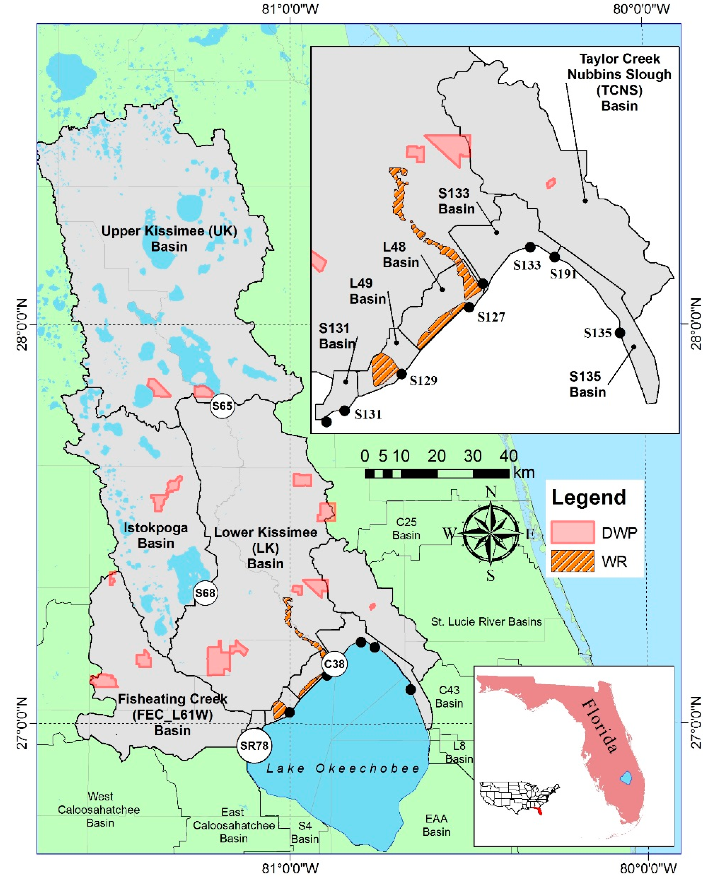
2.1. Study Area

The region of interest for the present study includes the northern basins contributing to LO inflows (Figure 1) with a total drainage area of ~10,600 km². The individual basins are (1) the Kissimmee Chain of Lakes/Upper Kissimmee (UK) basin, (2) the Lower Kissimmee (LK) basin, (3) the Lake Istokpoga basin, (4) the Fisheating Creek basin including the L61W drainage area (FEC_L61W), (5) Taylor Creek–Nubbin Slough (TCNS), (6) S135, (7) S133, (8) S131, (9) L48, and (10) L49. The Kissimmee River forms the main drainage channel in this area. There are several smaller creeks, sloughs, agricultural ditches, flood control canals, and structures that route runoff from this region to LO. The NLO region is well monitored for rainfall, flow, and water quality (details can be found on the South Florida Water Management District website https://apps.sfwmd.gov/WAB/EnvironmentalMonitoring/index.html). The average annual rainfall in UK is approximately 1255 mm, while the rest of the basins receive 1120 mm annually [24,25] with 70% of the rainfall occurring in the wet season (May to October). Correspondingly, most of the TP transport also takes place during the same period posing a challenge to non-point source TP management [26,27]. About 41.1% of the study area is under agricultural land use (

Table 1. Land use (LU) summary in the northern Lake Okeechobee watershed.

LU Category	Percent
Agriculture	41.1
Dairy and Animal Feeding Operations	0.7
Pastures	29.1
Improved Pasture	22.5
Unimproved Pasture	5.7
Woodland Pasture	0.5
Intensive Pasture	0.2
Others	0.1
Other Agriculture	11.3
Urban and Developed	13.4
Residential	10.8
Commercial, Industrial, and other Developed	2.6
Natural	45.5
Wetlands	19.4
Forests	7.3
Scrub, Brush, and Barren	10.8
Lakes, Streams, and Water Bodies	7.9

) with improved and unimproved cattle pastures covering 29.1% of the land cover. Other agricultural activities include citrus groves, sugarcane, row and field crops, sod farms, and tree plantations. Urban and developed areas cover 13.4% of this region and are predominantly located in the northern portion of UK basin around the Orlando metropolitan area. Wetlands cover 19.4% of the NLO basins along with 7.3% of forests and 7.9% of water bodies that include the Kissimmee Chain of lakes and Lake Istokpoga. Immokalee and Smyrna are the dominant soil types covering approximately 65% NLO basins’ extent. Both soils are Spodosols characterized by sandy texture, poor drainage, and low phosphorus retention capacity [28].

2.2. Watershed Modeling

The individual NLO basins were modeled for hydrologic and phosphorus water quality dynamics using the Watershed Assessment Model (WAM) [29]. The Base conditions (1998–2007) and three of the four restoration strategies considered in this study (BMPs, DWM, and WR) were modeled with WAM. The stormwater treatment area (STA) requirements to achieve a TP concentration target of 40 µg/L for each restoration scenario modeled in WAM was determined using the Dynamic Model for Stormwater Treatment Area (DMSTA) [30]. Both models have been widely used in Florida as decision support tools while formulating and evaluating alternatives for restoration plans [15,23,31,32,33,34].

2.2.1. Watershed Assessment Model: Model Setup and Re-calibration

WAM is a spatially distributed model designed to handle the hydrologic conditions typical to Florida (abundance of wetlands, high groundwater table conditions, hydric soils, canal networks that experience periodic flow reversals, and complex water control structure operations). These hydrologic conditions in south Florida are unique and, unlike WAM, most of the widely used watershed scale models (e.g., Soil and Water Analysis Tool, SWAT; Hydrologic Simulation Program FORTRAN, HSPF) fail to successfully simulate them [35]. WAM simulates the earthbound part of the hydrological cycle to calculate basin level flow and water quality dynamics [29]. Unique combinations of soil, land use, rainfall, irrigation, and waste utility zones are identified, grouped together, and simulated using one of the three source level models. The Everglades Agricultural Area Model (EAAMOD) [36] is used for agronomic crops on hydric soils while open water, mining, aquaculture, and wetlands are simulated using a simple water balance approach model called ‘Special Case’ developed for WAM [37]. EAAMOD was identified as the most appropriate field scale water quality model for agriculture on hydric soils in central and south Florida [38]. All other unique cell combinations are simulated using the Groundwater Loading Effects of Agricultural Management Systems model (GLEAMS) [39]. Daily flows and water quality constituents from these field scale models calculated at each grid cell (user defined, but typically and in this study 0.01 km²) are then adjusted for retention/detention (R/D) systems, if present, before routing simulated daily outputs to the stream network and ultimately to the watershed outlet. WAM uses six elevation-based flowpaths/distance grids to attenuate daily source level surface and sub-surface flows and loads accounting for features en route to the watershed outlet. Overland and in-stream water quality attenuation follows generalized exponential decay type equations (Equations (1) and (2)), respectively.

$$C_{out}=C_b+\left(C_{in}-C_b\right)e^{-\left(a{q}^{-b}\right)d}$$

(1)

$$C_{out}=C_b+\left(C_{in}-C_b\right)e^{-a\frac{\tau }{R}}$$

(2)

where C_b = background nutrient concentration (mg/L), C_out = outflow from flowpath (overland) or stream reach (instream) nutrient concentration (mg/L), C_in = inflow from source cell (overland) or upstream reach (instream) nutrient concentration (mg/L), a and b = empirical water quality attenuation exponent and multiplier, respectively (for in-stream attenuation b = 0), q = flow (m³ s⁻¹), d = overland flowpath distance (m), R = hydraulic radius of stream, τ = time interval.

A 10-year simulation period (1998–2007) was selected for this study to cover a range of conditions (wet and dry periods, see Figure S1 for details) prior to the implementation of any major water quality improvement project (e.g., BMPs) in the region, while maintaining longevity of the study. WAM has been already used to model the NLO basins in phosphorus budget analysis studies [26,40,41]. These existing model setups were obtained from the SFWMD (personal communication) for all basins shown in Figure 1, except the UK setup, which was obtained from [42]. The above listed studies have detailed information on WAM input datasets used in the modeling (land use, soil, rainfall, hydrography, elevation, water control structures and their operations, etc.). Re-calibration was performed for all the individual basins through minor adjustments to the location of the calibration gauges, evapotranspiration, and phosphorus attenuation exponent and multiplier parameters for streams and dominant land uses [35,43] to account for marginally different simulation periods in earlier studies (1999–2007 in [40] and 2002–2007 in [42]). Two goodness of fit (GOF) measures, Nash–Sutcliffe Efficiency (NSE) Equation (3) and Percentage Bias (PBIAS) Equation (4), were calculated for monthly flows and TPL at 10 locations (one gauge per basin) [44] (Figure 1). While NSE is a good indicator of ability of the model to capture long-term hydrologic and water quality dynamics, PBIAS is a good measure of the model deviation and of the average model behavior. Both these GOFs are recommended evaluation measures by the American Society of Agricultural and Biological Engineers standards on hydrologic and water quality modeling guidelines [45] with clearly defined criteria for model performance classification. Since the focus of this study was to assess the relative change in average flows and TPL along with an economic valuation of restoration alternatives, re-calibration was performed considering the entire simulation period.

$$NSE=1-\frac{{\sum }_{i=1}^N{\left(O_i-P_i\right)}^2}{{\sum }_{i=1}^N{\left(O_i-\overline{O}\right)}^2}$$

(3)

$$PBIAS=\frac{{\sum }_{i=1}^N\left(O_i-P_i\right)}{{\sum }_{i=1}^N{O}_i}\times 100$$

(4)

where N = number of time steps, O_i = observation at the ith time step, P_i = simulated value at the ith time step, Ō = mean of observations.

2.2.2. Dynamic Model for Stormwater Treatment Area (DMSTA)

The DMSTA2 is a transient wetland flow and phosphorus cycling model used to design treatment wetlands [30,46]. Daily timeseries of rainfall, evapotranspiration, inflow, and phosphorus concentration constitute DMSTA2 inputs while wetland size, hydraulics, and vegetation type constitute primary design variables. Treatment areas are typically divided into cells connected in series or parallel pathways forming a treatment network. Phosphorus dynamics is simulated considering soil, biota, and water column components. Inter-compartmental fluxes, uptake, and release of phosphorus by vegetative biomass are accounted through simplified processes. The vegetation-specific calibration parameters for DMSTA2 have been developed for different vegetation types using data from full-scale STAs, lakes, reservoirs, and natural wetlands in south Florida [46,47]. DMSTA2 is a reliable STA design and restoration alternatives evaluation tool used by state and federal agencies [32,33,48]. In this study, STA inflow and phosphorus concentration timeseries were created by combining the daily WAM outputs (flow and phosphorus concentration timeseries) at the basin outlets. Rainfall and evapotranspiration timeseries were defined based on measurements in this region.

2.3. Restoration Scenarios

Twenty restoration alternatives/scenarios (including Base) were formulated by combining four phosphorus control strategies (BMP, DWM, WR, and STA). The salient features and corresponding WAM parameterization of these restoration strategies are described below. BMP types and DWM parameterizations were applied uniformly across respective land uses in all NLO basins. It is noteworthy that identification of pollution hot-spots and performing spatial optimization of BMPs has been demonstrated in many recent modeling studies (e.g., [49,50,51,52,53]). However, due to the large size of the investigated region (10,600 km²) and focus on overall restoration cost to achieve TMDL, no explicit spatial optimization of these restoration strategies was performed. TP loading hot-spots were identified for this region (Figures S2 and S3, Table S1) and were found to be consistent with previous studies [26,40,42]. The analysis presented in this work can be used as a starting point for further optimization of restoration projects.

2.3.1. Best Management Practices

Best Management Practices (BMPs) implemented in NLO basins have been classified into three types [54,55]. Type I BMPs are implemented by the producer/land owner, typically at a low cost, and primarily involve nutrient management actions (e.g., fertilizer selection, application rate and timing, record keeping) [56]. Type II BMPs require structural modifications (fencing, wetland/stormwater R/D, improved irrigation system) and are typically funded through cost-share programs (after the producer/landowner had already implemented type I BMPs). Type III BMPs are more expensive and involve edge of the field stormwater R/D with chemical technologies, e.g., aluminum sulphate and iron chloride, etc. (after the producer/landowner had already implemented types I and II BMPs) [57]. Based on these BMP types, three levels of restoration—(1) BMP1 = Type I, (2) BMP12 = Type I + Type II, and (3) BMP123 = Type I + Type II + Type III—were considered. BMP parameterization for land uses in the NLO basins are summarized in

Table 2. Summary of WAM parameterization for restoration strategies (a) Best Management Practices (BMP), and (b) Disperse Water Management (DWM).

Land Use	Percent P Fertilizer Reduction	Water Management	Increase in Retention/Detention (m3/ha)	Percent P Reduction under Other Type II BMPs	Percent Reduction under EOF Chemical Treatment and Other Type III BMPs	Increase in Storage (m3/ha)
						LRD	HRD
	Type I	Type II	Type II	Type II	Type III	DWM
Citrus	12	N	260	0	45	0	0
Commercial and Services	10	N	40	0	0	0	0
Coniferous Plantation	33	N	50	0	50	0	0
Dairies	100	Y	300	0	50	0	0
Field Crops	20	Y	200	0	40	0	0
Fruit Orchards	30	N	100	0	0	0	0
High Density Residential	30	N	100	0	65	0	0
Improved Pasture	100	N	100	5	50	100	600
Industrial	5	N	100	0	0	0	0
Intensive Pasture	100	N	100	5	50	100	600
Low Density Residential	25	N	250	0	65	0	0
Managed Landscape	10	N	100	0	0	0	0
Medium Density Residential	30	N	100	0	65	0	0
Multiple Dwelling Units	30	N	100	0	65	0	0
Ornamental Nurseries	30	N	1000	5	50	0	0
Row Crops	30	Y	300	0	50	0	0
Sod Farms	20	Y	250	0	50	0	0
Sugarcane	30	Y	400	0	50	0	0
Transportation Corridors	100	N	40	0	0	0	0
Tree Nurseries	30	Y	150	0	0	0	0
Unimproved Pasture	100	N	30	2	45	100	600
Woodland Pasture	100	N	10	2	40	100	600

. While BMPs are formulated and implemented for phosphorus as well as other nutrients, only the phosphorus-related practices were the focus of this study. Fertilization rates, irrigation control, culvert operations, and wetland/stormwater R/D BMPs were simulated mechanistically. Effects of all other BMPs (at the field scale), which included buffer strips, critical area fencing, edge of the field chemical treatment, etc., were incorporated in the model by adopting BMPs effectiveness factors, i.e., phosphorus reduction factors [54]. Not all individual BMPs were applied to all land uses and their categorization into type I, II, and III also differed in some cases. Additional details on BMPs can be found in the literature [54], which was used as the basis for BMP scenario formulation.

2.3.2. Dispersed Water Management

Dispersed Water Management (DWM) is a practice to retain water on private or public lands using existing or minimal new infrastructure to facilitate restoration efforts in the Northern Everglades [58]. Apart from providing dispersed storage, some DWM projects can help improving water quality (nutrient retention in wetlands) while also providing improved ecological habitat [59,60]. In this work, three types of DWM alternatives were considered. The first alternative was based on existing projects and the remaining two alternatives were based on hypothetical R/D levels. DWM was modeled using depth-based wet stormwater R/D ponds. WAM calculates daily runoff and percolation from the pond based on a water balance approach (rainfall, evapotranspiration, percolation). Nutrient outflow concentrations are calculated using wetland attenuation parameters with stream routing algorithm Equation (2).

As of 2016, there were 21 dispersed water projects (DWPs) operating or under construction in the study area (Table S2), estimated to provide a total of 34 × 10⁶ m³ of average annual storage using the Potential Water Retention Model (PWRM) developed by the [60,61]. Corresponding R/D pond parameters (storage ratio and pond depth) were inversely quantified to match the PWRM estimates for annual flow reductions [61]. In this study, DWPs were modeled as an alternative since most of the DWPs within the study area, located on privately owned pasturelands [62], were built after 2007. This concept of using pastures for water storage was extended to create two hypothetical DWM levels, (a) Low Retention/Detention (LRD) and (b) High Retention/Detention (HRD). LRD and HRD alternatives were applied to improved, unimproved, woodland, and intensive pastures land uses (covering 29% of the NLO watershed area). Storage ratio and pond depths were defined based on prior studies (e.g., [40]) and expert opinion (D. Bottcher, SWET Inc., personal communication) to determine the practically viable setting for agricultural stormwater R/D. This parameterization translated to approximately 1% and 6% of pastureland being converted to R/D ponds of 0.5 m depth for DWM purposes under LRD and HRD, respectively.

2.3.3. Wetland Restoration

Wetland Restoration (WR) involves rehydration of drained wetlands to provide storage, nutrient assimilation, habitat improvement for wetland wildlife, and creating recreation opportunities. Historically, wetlands covered a large area of the NLO watershed, much of which was converted into agricultural land in the 20th century. However, under present land use, it is neither feasible nor possible to restore all pre-development wetlands. State and federal agencies shortlisted four areas for WR projects through a multi-criteria selection process, namely (a) Kissimmee River Wetlands (LK basin), (b) Paradise Run Wetlands (LK and L48 basins), (c) Lake Okeechobee West Wetlands (L48 basin), and (d) IP-10 Wetlands (L49 basin), cumulatively covering an area of 52 km² [63]. These four projects constituted one WR alternative in this study. WAM uses ‘Special Case’ sub-module to simulate wetlands by maintaining the complete water balance based on rainfall, evapotranspiration, crop coefficient, percolation, and maximum inundation depth [29]. Nutrient concentrations in runoff are calculated based on user specified event mean concentrations (EMC) for each wetland type. WR projects were parameterized in WAM by first changing all land uses within WR project areas to wetland and setting a maximum inundation depth to 2 m to mimic the common wetland parametrization in WAM [37], thus increasing storage capacity and hydroperiod.

2.3.4. Stormwater Treatment Area

Stormwater Treatment Areas (STAs) were sized to meet a long-term annual TP flow weighted mean concentration (FWMC) of 40 µg/L at the LO inflow, a TP level similar to the LO pelagic zone TP concentration goal [21]. Walker and Havens [17] showed how the relationship between near-shore TP concentration of 40 µg/L and algae bloom frequency was used to derive this goal. Two assumptions were made when designing the STAs: (1) STAs were to be located close to LO to avoid prolonged ‘no flow’ periods, a major STA maintenance aspect [47] and (2) outflows could be diverted from NLO basins to the STA locations, thus enabling the grouping of the basin WAM outflows and TPLs and restrict the number of STAs to a lower number (five for this analysis). No further analysis about land availability or suitability was performed. Previous STA design studies have indicated that phosphorus removal efficiency is size dependent with very small treatment areas not working optimally [64]. Each STA was designed as a network of 3 to 5 parallel pathways, with each pathway consisting of an emergent aquatic vegetation cell followed by a submerged aquatic vegetation cell. Such a design has been found effective in removing phosphorus [48]. Currently, there are three working STA projects located in the TCNS (0.6 and 3.2 km²) and S135 (3.7 km²) basins with a total effective treatment area of 7.5 km² designed to remove 16.1 mtons of TPL. Though two of these STAs in the TCNS became operational around 2007 (designed to remove 7.1 mtons of TPL), they have been facing operational challenges, while only the first phase of the third STA, known as Lakeside Ranch STA, (designed to remove 9.1 mtons of TPL) was completed in 2013. The second phase of Lakeside Ranch STA (~3.3 km²), designed to remove 10 mtons of TPL annually, is anticipated to become fully operational in 2020 [15]. Hence, the three STAs were not incorporated in the Base scenario, while impact of only the Lakeside Ranch STA was demonstrated for the optimal restoration scenario selected in this study. The Lakeside Ranch STA was considered in this study because of its high TPL removal performance and of its location close to LO to avoid prolonged ‘no flow’ periods, a main assumption of the present study.

2.4. Cost Model

The cost of implementing different combinations of BMPs, DWM, WR, and STAs to achieve the LO inflow TP FWMC of 40 µg/L were determined to find the most cost-effective restoration scenario. The following cost minimization equations were used (Equations (5) and (6)):

$$\begin{array}{l}Min\left(Z\right)={\displaystyle \sum _{n=1}^3}{\displaystyle \sum _{i1=1}^{22}}{C}_{i1,n}^B{L}_{i1,n}{A}_{i1,n}\\ \hspace{1em}\hspace{1em}\hspace{1em}\hspace{1em}\hspace{1em}\hspace{1em}\hspace{1em}+{\displaystyle \sum _{m=1}^2}{\displaystyle \sum _{i2=1}^4}{C}_{i2,m}^{D1}{L}_{i2,m}{A}_{i2,m}+{\displaystyle \sum _{j=1}^{21}}{C}^{D2}{V}_j+{\displaystyle \sum _{k=1}^5}{C}^S{L}_k+{\displaystyle \sum _{l=1}^4}{C}_l^W\end{array}$$

(5)

FWMC TP ≤ 40 µg/L

(6)

Subjected to the constraint:

Where i1 = land use type, n = BMP type (I, II, III), $C_{i1,n}^B$ = unit cost of BMP ($/kg/acre/year) type n and for land use i1, $L_{i1,n}$ = TPL reduction (kg) from land use i1 for n types of BMPs, $A_{i1,n}$ = area (acres) for land use i1 and n types of BMPs, i2 = land use type for DWM, m = DWM type (LRD, HRD), $C_{i2,m}^{D1}$ = unit cost of DWM ($/kg/acre/year) for DWM type m and land use i2, $L_{i2,m}$ = TPL reduction (kg) from land use i2 for DWM type m, $A_{i2,m}$ = area (acres) for land use i2 for DWM type m, j = DWP project index (1 to 21), $C^{D2}$ = unit cost of DWP ($/acre-ft/year), V_j = runoff storage volume (acre-ft) for DWP project j, k = STA project index (1 to 5), C^S = unit cost of STA ($/kg of TP removed/year), L_k = TP Load reduction (kg) by STA project k, l = WR project index (1 to 4), and $C_l^W$ = cost of WR project l ($/year). Since project durations assumed in unit cost estimations differed from one another, all costs were converted to 2014 dollars using the Consumer Price Index (CPI) from the Bureau of Labor Statistics and were discounted using a 4% real discount rate.

The effectiveness of BMP implementation and hence the cost is spatial in nature (due to land use and soil variability) and was incorporated into the cost estimation model by quantifying the TPL reduction from individual land parcels in WAM. The unit costs for BMPs (

Table 3. Summary of unit costs associated with Best Management Practices ¹.

Land Use	Project Type	Amortized Capital Cost ($/kg of TP removed/acre/year)	Amortized O&M Cost ($/kg of TP removed/acre/year)	Total Annual Cost 2 ($/kg of TP removed/acre/year)
Citrus, Fruit Orchards	Type I	0.0	0.0	0.0
	Type II	98.5	24.6	153.9
	Type III	147.7	36.9	230.8
Commercial, High Den. Res., Med. Den. Res., Low Den. Res., Multi-Dwelling, Industrial, Transportation Corridors	Type I	0.0	0.0	0.0
	Type II	5904.8	1476.2	9226.2
	Type III	2699.1	674.8	4217.3
Conifer	Type I	0.0	0.0	0.0
	Type II	1439.6	359.9	2249.4
	Type III	460.0	115.0	718.7
Dairies	Type I	9.1	2.3	14.2
	Type II	409.5	102.4	639.8
	Type III	141.2	35.3	220.7
Field Crops	Type I	16.8	4.2	26.3
	Type II	35.0	8.7	54.7
	Type III	70.0	17.5	109.3
Improved Pasture, Intensive Pasture	Type I	57.0	14.3	89.1
	Type II	116.6	29.2	182.2
	Type III	129.6	32.4	202.5
Ornamental Nurseries, Tree Nurseries	Type I	3.9	1.0	6.1
	Type II	60.9	15.2	95.2
	Type III	89.4	22.4	139.7
Row Crops	Type I	2.6	0.6	4.0
	Type II	45.4	11.3	70.9
	Type III	58.3	14.6	91.1
Sod Farms	Type I	5.2	1.3	8.1
	Type II	66.1	16.5	103.3
	Type III	108.8	27.2	170.1
Sugarcane	Type I	0.0	0.0	0.0
	Type II	308.4	77.1	481.9
	Type III	348.6	87.1	544.6
Unimproved Pasture	Type I	27.2	6.8	42.5
	Type II	72.6	18.1	113.4
	Type III	106.3	26.6	166.0
Woodland Pasture	Type I	84.2	21.1	131.6
	Type II	281.2	70.3	439.3
	Type III	241.0	60.3	376.6
Managed Landscape	Type I	5.2	1.3	8.1
	Type II	66.1	16.5	103.3
	Type III	108.8	27.2	170.1

¹—BMP unit costs are based on [54] Letter Report. Total project cost (2014 present value) is calculated assuming 4% discount rate and 20-year project period. ²—Total annual cost includes contingency cost (25% of Initial and O&M costs).

) were based on [54]. The average storage-based payment rate for projects on private ranchlands were used to determine the costs of DWPs [58]. Considering the uncertainties in potential storage estimates [65,66] and the fact that the LRD and HRD projects modeled in this work were aimed at TPL reduction assessment instead of runoff storage, stormwater R/D BMP unit costs were used for LRD and HRD cost evaluation. WR project costs were adopted from [67] preliminary cost estimates. The determination of the STA costs was based on the costs of two STA projects in the TCNS basin completed in the late 2000s and reported in [68]. Land acquisition cost was updated to $15,000/acre based on more recent estimates of land cost [69].

Table 4. Summary of costs associated with Disperse Water Management (DWM), Stormwater Treatment Areas (STA), and Wetland Restoration (WR).

Restoration Strategy	Land Use	Project Type	Amortized Capital Cost	Amortized O&M Cost	Total Annual Cost 1
DWM	Improved and Intensive Pasture	LRD, HRD 2	168.4	42.1	263.2
	Unimproved Pasture	LRD, HRD	268.2	67.1	419.1
	Woodland Pasture	LRD, HRD	338.2	84.5	528.4
	N.A.	DWP 3			297.9
STA 4			448.4	112.1	700.5
WR 5					3265.3

¹—Total Annual cost includes contingency. ²—LRD and HRD unit costs ($/kg of TP removed/acre/year) are P reduction based costs, estimated based on R/D BMP in [54] Letter Report. Assumed project duration = 20 years, contingency = 25%, and discount rate = 4%. ³—DWP unit costs ($/acre-ft of runoff reduced/year) are based on payment rates for existing Disperse Water Management Projects on public ranchlands [58]. Assumed project duration = 10 years, contingency = 25%, and discount rate = 4%. ⁴—STA unit costs ($/kg of TP removed/year) are based on actual Taylor Creek and Nubbin Slough STA project costs (updated for land acquisition). Assumed project duration = 50 years, contingency = 25%, and discount rate = 4%. ⁵—WR unit costs ($/acre/year) are based on estimates presented in Lake Okeechobee Watershed Restoration Project [67]. Assumed project duration = 20 years, discount rate = 4%. Since [67] estimates included contingency costs, no further contingency was added.

reports unit costs and other related assumptions for DWM, STA, and WR.

To reduce the number of combinations and permutations of the different phosphorus control strategies, a phased assessment approach was adopted in this study (Figure 2). First, WAM re-calibration was performed to establish the Base scenario. In Phase I, the three BMP scenarios—BMP1, BMP12, and BMP123—were assessed. In Phase II, the most cost-efficient scenario of Phase I was considered to build five new scenarios based on DWP and DWM projects. Very large cost differences between Phase I scenarios (details presented in Results) made this approach justifiable. In Phase III, one new scenario was formulated by combining the most cost-efficient Phase II scenario with WR projects. Each of these scenarios were evaluated with and without STAs. From the potential 100+ different combinations, this phased approach reduced the total investigated scenarios to 20, thus also reducing the model simulation resource requirements.

3. Results

3.1. Watershed Modeling and TP Reduction Strategies

3.1.1. Re-calibration

A summary of the NLO basin re-calibration GOF results is presented in

Table 5. Re-calibration summary of northern Lake Okeechobee watershed basins.

Basin	Area (km2)	Re-Calibration Location	Monthly Flow		Monthly TPL
			NSE	PBIAS	NSE	PBIAS
S131	28.9	S131	0.49	7%	0.26	10%
L48	84.0	S127	0.58	−3%	0.45	12%
L49	48.9	S129	0.56	−8%	0.32	8%
S133	103.8	S133	0.84	−1%	0.81	9%
S135	73.2	S135	0.67	−7%	0.58	8%
FEC_L61W	1205.0	SR78	0.33	7%	0.49	4%
Istokpoga	1578.6	S68	0.54	5%	not enough data
Taylor Creek-Nubbin Slough	487.0	S191	0.79	11%	0.78	19%
Upper Kissimmee	4162.8	S65	0.36	−4%	0.48	−7%
Lower Kissimmee	2810.9	C38	0.94	−2%	0.68	−6%

. NSE values for monthly flows varied between 0.33 (SR78) to 0.94 (S65) with a mean NSE of 0.61 (arithmetic average of individual NSEs). The NSE values for monthly TPLs ranged between 0.26 (S131) and 0.81 (S133) with a mean NSE of 0.54. PBIAS for monthly flows varied between −8% (S129) and +11% (S191) (mean PBIAS = +0.5%), while monthly TPLs PBIAS was in the range −7% (S65) to +19% (S191) with a mean PBIAS of +6%. If we were to classify WAM simulation performance based on the recommendations of [44,45] for acceptable modeling results (NSE Flow > 0.5, NSE TPL > 0.35; abs(PBIAS Flow) < 15%, abs(PBIAS TPL) < 30%), three basins (S131, FEC_L61W, and UK) would have simulated flows with unsatisfactory NSEs, and two basins (S131 and L49) would have simulated TPLs with unsatisfactory NSEs. In all cases, the corresponding PBIAS values were well within the acceptable limit indicating that WAM was not able to satisfactorily capture flow or TPL dynamics at those locations but was able to simulate the average system behavior over the period of study. Since the purpose of this study was to assess the average TPL reductions under different scenarios, usage of the re-calibrated WAM setups were justified for this exploratory feasibility study.

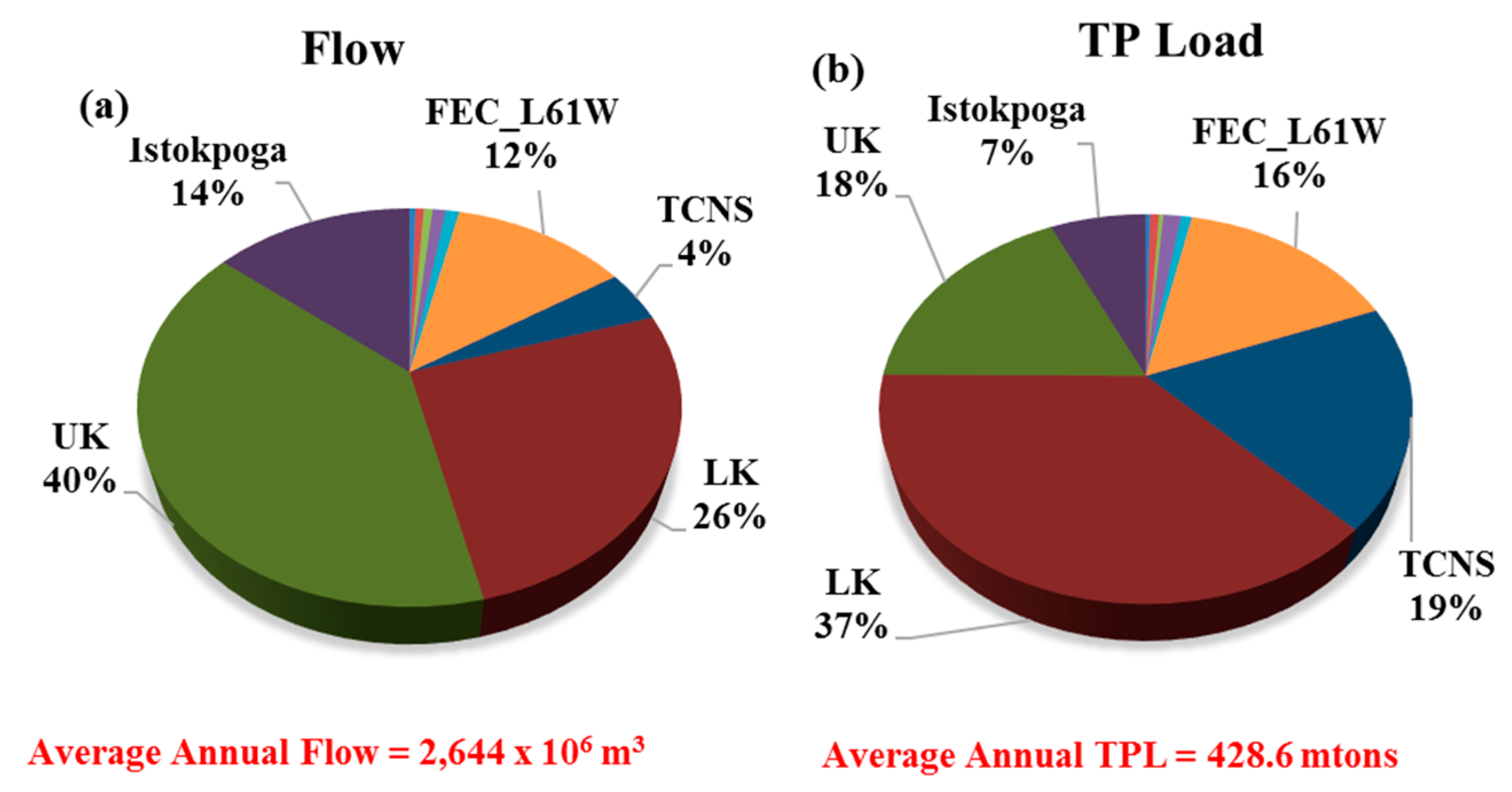
3.1.2. WAM Results for the Base and Restoration Scenarios

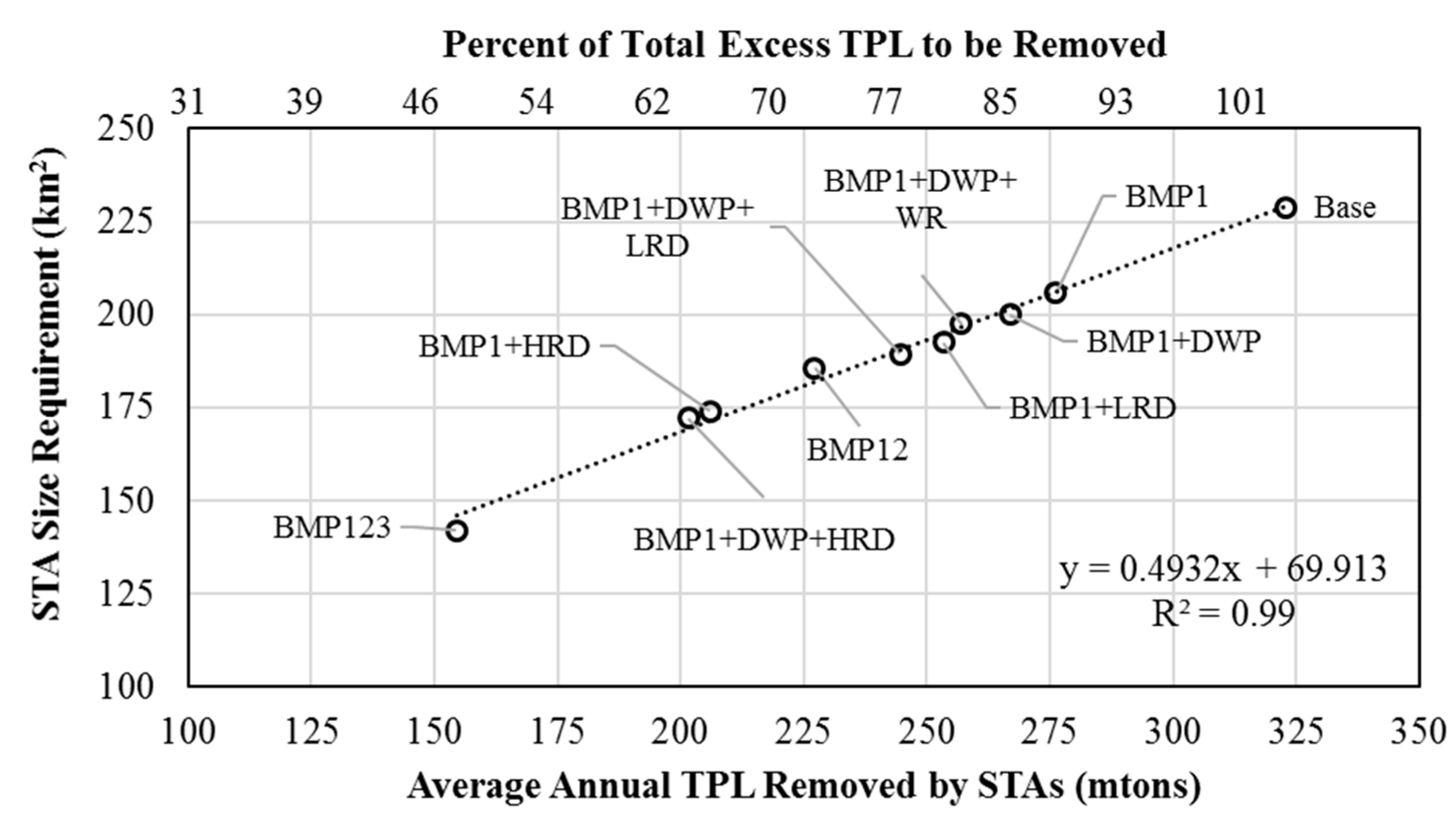
The re-calibrated Base scenario simulation results indicated that the NLO basins contributed an annual average of 2644 × 10⁶ m³ of flows and 428.6 mtons of TPL to LO during 1998–2007 (Figure 3a,b). The two largest NLO basins (UK and LK) contributed 40% and 26% of the total water inflows to LO, respectively, while their TPL contributions were 18% and 37%, respectively. The TCNS basin contributed 4% of the total flows to LO and was responsible for 19% of the TPL. These results are consistent with the monitoring data and with previous modeling efforts showing that TCNS, S154, S65E, S65D, and Indian Prairie basins (the latter four are part of LK in this study) are the highest TP contributors to LO in terms of load per unit area [15,70]. Figure 4 summarizes flows, TPLs, and FWMC for the Base and restoration scenarios, pre-STA values. The Base scenario inter-annual variability at LO inflows was large with flows ranging from 749 × 10⁶ m³ to 4436 × 10⁶ m³ (Figure 4a), TPLs ranging from 95 mtons to 675 mtons (Figure 4b), and FWMC ranging from 124 µg/L to 286 µg/L (Figure 4c) with an average of 173 µg/L. The reduction in flows and TPLs (%) when compared to the Base conditions are also presented on the secondary vertical axes of Figure 4a,b.

Under the restoration scenarios, flows ranged between 2644 × 10⁶ m³ (BMP1) and 2515 × 10⁶ m³ (BMP1+DWP+HDR) indicating that flows reduced by less than 5% relative to the Base scenario (Figure 4a). The BMP123 scenario resulted in the highest TPL reduction (39.3%) with a TPL contribution of 260 mtons to LO (Figure 4b). The second and third best scenarios in terms of TPL reduction were BMP1+DWP+HRD and BMP1+HRD with an average annual TPL of 307 mtons (28.3% reduction) and 312 mtons (27.3% reduction), respectively. TPL reduction for the other six scenarios ranged between 11% and 22.3%. Under the Base scenario, the annual average inflow TP FWMC to LO was 173 µg/L, 4.3 times the target value of 40 µg/L (Figure 4c). Under the restoration scenarios, changes in FWMCs followed the reduction in TPLs. BMP123 contributed inflows to LO at 105 µg/L (2.6 times the target), the lowest among all scenarios. Under this scenario, the TP target concentration of 40 µg/L could not be achieved even for a single year. For the other scenarios, annual average FWMC ranged between 130 and 154 µg/L.

3.1.3. STA Sizing

WAM results indicated that restoration scenarios using BMPs, DWM, and WR were not sufficient and STAs are necessary to achieve the target inflow TP concentration for LO. The total STA size requirement ranged from 142 km² for the BMP123 scenario and 229 km² for the Base scenario with the corresponding average annual TPL reduction ranging from 155 and 323 mtons, respectively (Figure 5). The other restoration scenarios required STAs within a relatively narrower area range of 172 to 206 km². The STA size requirement in the NLO region is comparable to the currently operating STAs south of LO covering an area of approximately 227 km². Figure 5 also indicated a good linear relationship (R² = 0.99) between the average annual TPL removal and STA sizes. The same figure also shows that under the BMP123 scenario, STAs contributed 48% to the TPL removal requirement while the relative STA contribution was more than 60% for all other scenarios, indicating the importance of the STA technology in LO water quality restoration.

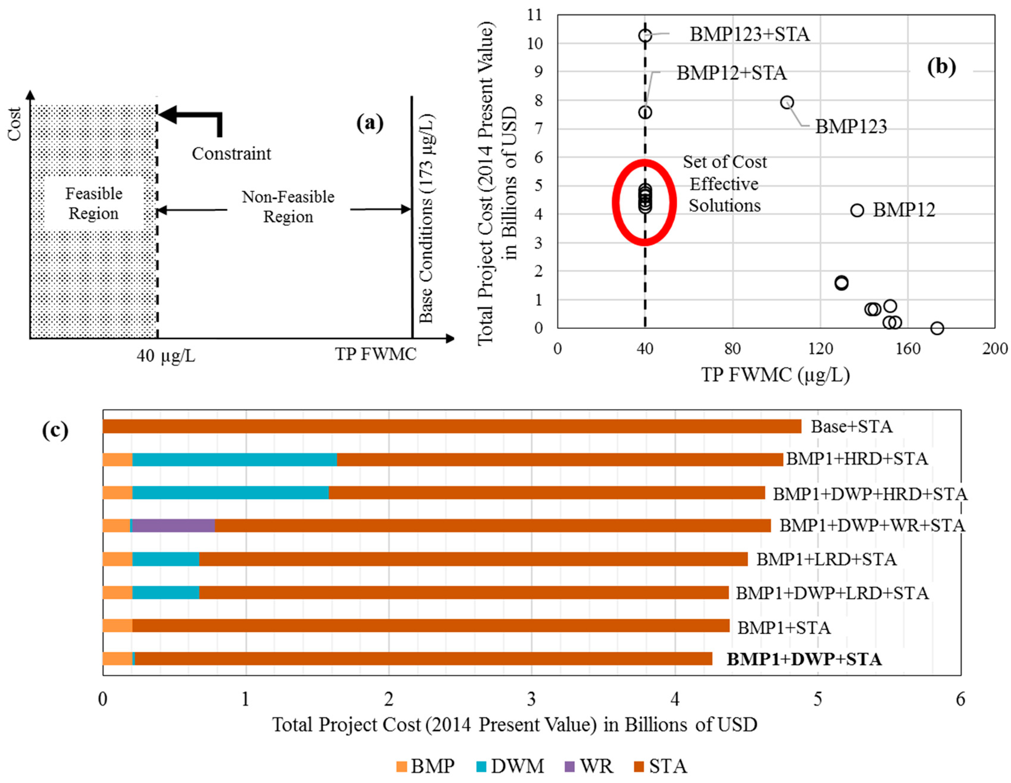
3.2. Assessment of Cost-Effectiveness

The schematic of this restoration scenario-based project cost-effectiveness assessment is shown in Figure 6a. The only constraint used for minimizing the costs was the attainment of the LO inflow TP target of 40 µg/L, making the area to the left of the vertical line the only “feasible region” (shaded area). In other words, any scenario laying to the right side of the constraint line is an unacceptable combination of restoration strategies. As previously noted, scenarios based on combining BMPs, DWMs, and WR alone could not reduce TP concentrations to or below 40 µg/L. Accordingly, all these scenarios were placed in the non-feasible region (Figure 6b), while the scenarios with STAs fell on the constraint line to form a set of feasible solutions. However, the total costs varied substantially from one scenario to another. The highest total costs (2014 present value) were estimated around US $7.6 and $10.3 billion for BMP12+STA and BMP123+STA, respectively. The remaining eight scenarios with STAs had total costs varying in a relatively narrow range (US $4.26 to 4.75 billion), forming a set of cost-effective feasible solutions. The high pre-STA costs of BMP12 and BMP123 implementation (~US $4.1 and $7.9 billion, respectively) justified the phased approach adopted in this work.

The BMP1+DWP+STA was determined as the most cost-efficient scenario among the ones investigated in this study with a total cost of US $4.26 billion. The cost breakdown (Figure 6c and

Table 6. Relative contributions of restoration strategies to TPL removal and Total Project Cost.

	% Total TPL Reduced				% Total Project Cost
	BMPs	DWM	WR	STAs	BMPs	DWM	WR	STAs
BMP1+DWP+STA	14.5	2.9	0.0	82.7	4.8	0.4	0.0	94.8
BMP1+STA	14.5	0.0	0.0	85.5	4.6	0.0	0.0	95.4
BMP1+DWP+LRD+STA	14.5	9.8	0.0	75.8	4.6	10.8	0.0	84.6
BMP1+LRD+STA	14.5	7.1	0.0	78.5	4.5	10.4	0.0	85.1
BMP1+DWP+WR+STA	14.5	2.9	3.0	79.6	4.0	0.4	12.4	83.2
BMP1+DWP+HRD+STA	14.5	23.1	0.0	62.5	4.4	29.7	0.0	66.0
BMP1+HRD+STA	14.5	21.7	0.0	63.8	4.3	30.2	0.0	65.6
Base+STA	0.0	0.0	0.0	100.0	0.0	0.0	0.0	100.0

) indicated that type I BMPs, DWP (existing dispersed water management projects), and STAs (200 km²) were responsible for 4.8% (US $0.2 billion), 0.4% (US $17 million), and 94.8% (US $4.04 billion) of the total project cost, respectively. The corresponding TPL removal contributions of those restoration strategies were 14.5% (46.7 mtons), 2.9% (9.3 mtons), and 82.6% (267 mtons), respectively. For all other BMP-based feasible scenarios, type I BMPs contributed around 14.5% to the required TPL removal while the associated cost was relatively lower (4.0 to 4.8%). The relative TPL removal and cost of DWM varied substantially among scenarios (2.9 to 23.1% and 0.4 to 30.2%, respectively) depending on the type of DWM. The relatively high cost (65.6 to 100%) and TPL removal contribution (62.5 to 100%) of STAs to the overall project indicate the importance of accurately estimating the STA size and the associated unit cost of TP removal.

It is worth noting that there is a cost estimation uncertainty on all the projects listed above depending on the cost methodology adopted. For the DWM cost calculation, there is an additional uncertainty associated with the runoff reduction volume calculations using PWRM for DWP, for example, [71] raised concerns about the accuracy of PWRM. Based on modeling studies, albeit restricted to only a few wetland-pasture study sites in south Florida, [72] and [66] showed that storage estimates are highly sensitive to wetland evapotranspiration and topographic data. These parameters are not fully or adequately included in the inputs of PWRM model. Consequently, the actual payment rates for water storage do not use accurate storage estimates. Goswami and Shukla [65] concluded that the actual storage potential in NLO basins through dispersed storage (i.e., wetland restoration on ranchlands) is only about 14% of the required storage estimated by the state agencies. Runoff reduction achieved under BMP1+LRD scenarios in the present study was similar to the storage projections in [65]. In this work, DWM (i.e., LRD and HRD) was explored as phosphorus control strategy rather than using it for creating water storage. Hence, the corresponding cost calculations were based on TPL reduction potential i.e., stormwater R/D BMP rates. For a large-scale implementation of DWM projects in the NLO basin, a detailed feasibility study of DWM storage efficiency, nutrient removal, and costs are required.

The most cost-effective scenario identified in this work consisted of (a) implementation of nutrient/fertilizer management BMPs throughout the NLO region, (b) continuation of existing NLO DWM projects, and (c) construction of 200 km² STAs for a total project cost of ~US $4.26 billion (2014 present value). Taking into account the Lakeside Ranch STA with an effective treatment area of 7 km², there is a need for 193 km² of STAs with a total project cost of $4.15 billion for future STAs needs + BMP type I + existing DWM projects.

4. Discussion

4.1. Current State Action Plan and the Present Study Implications

The 2014 BMAP is a restoration roadmap for water quality improvements in the NLO basin [73]. It details projects being (since 2009) or to be implemented to improve LO water quality and develops a monitoring strategy to track improvements. The plan is to follow a phased implementation of the strategies to achieve the LO TMDL. During the first phase of the BMAP, the projects are spread over a ten-year timeframe with a projected TPL reduction of 148 mtons (around 43% of the total necessary TP reduction to achieve the TMDL). Around 59 mtons of the expected TPL reductions will come from implementation of type I (31 mtons TPL reduction) and type II (28 mtons TPL reduction) BMPs. TPL reduction attributed to BMP implementation before 2009 was not accounted for in the BMAP. The other BMAP projects listed were DWM, WR, and STAs providing 19 mtons, 24 mtons, and 30 mtons of additional TPL reductions, respectively. The remaining 16 mtons of TPL removal would be through other treatment technologies. In this first BMAP phase, 40% of the expected TPL reduction will be originating from implementing BMPs with no long-term vision of how the Lake Okeechobee TMDL would be achieved.

Xu et al. [74] developed a procedure to determine the economic efficiency of conservation practices to reduce TPLs from the Sandusky watershed to Lake Erie and concluded that relying on traditional conservation practices alone is not sufficient in meeting the phosphorus targets. Gaddis et al. [75] investigated the TPLs from the Stevens Brook watershed and demonstrated that the maximum achievable annual phosphorus load reduction for the watershed is 46%, a significant step (but not enough) toward achieving the TMDL. These results are consistent with the findings of this paper demonstrating that STAs (above and beyond standard BMPs) would need to be implemented to reach the target. There is a need to establish a NLO procedure to assess the effectiveness and cost efficiency of nutrient control strategies using a holistic temporal and spatial approach.

Based on the current technologies (BMPs, DWM, WR and STAs), this paper assessed the most cost-effective plan to reach the LO target. The total cost of the most cost-effective plan would be around US $4.26 billion. This total estimate is substantially greater than the state of Florida agencies funding requests and expenditures in this watershed. Since 2000 to date, the State spent a total of around US $200 to $300 million [15,76]. In the BMAP document and excluding the Kissimmee River restoration, the total cost for reducing the TPL to LO by 43% was around $151 million with many features having unknown costs [73]. Based on the present study, the total cost for full implementation of BMP1 and BMP12 are around US $203 million and US $4 billion, respectively. A realistic estimate of the long-term total costs for reaching the LO TMDL needs to be developed and peer reviewed. This should be done along with an evaluation of the return on investment by quantifying the ecosystem services that a restored watershed would bring to the economy [77]. The high cost for restoring LO should not halt or delay restoration progress. To the contrary, state agencies should incentivize innovative practices to decrease/offset the cost of local and regional efforts to remove TP from surface waters, e.g., bioenergy production and novel landscape management [78,79,80], without delaying the immediate implementation of TP removal strategies delineated above. Finding knowledge gaps and incentivizing research and development in this area is critical to surpass the current level of treatment and lower capital and operational costs.

4.2. Challenges

An important challenge that was not accounted for in this study is the problem of legacy phosphorus in the NLO basins [81] directly impacting the time lag for observing any decreased water quality trend in the watershed. Hence the timeframe for improved inflow TP concentrations through the implementation of restoration strategies (with the exception of STAs) should not be interpreted as 10 years. Reddy et al. [82] estimated that phosphorus built-up in LO basin soils is enough to sustain ~500 mtons/year of TPL to LO for at least 22 to 55 years even after complete curtailment of all other phosphorus input sources. Phosphorus enriched sediments within LO are also likely to sustain high TP concentrations in the lake for 1 to 3 decades beyond the basin legacy phosphorus removal timeline. Similarly, other freshwater bodies in the NLO basin that are currently still assimilating phosphorus may become sources of phosphorus once their sediments reach a phosphorus sorption capacity through sustained high inflow TPLs or would buffer outflow TP concentrations from declining until an equilibrium is reached with the lowered inflow loads [55]. For example, [83] showed that the Kissimmee Chain of Lakes and Lake Istokpoga would become sources of TP in 7−25 years under 0 to 25% inflow TPL reductions. This means that restoration success is mainly dependent on STAs during the first years of any water quality project implementation in the NLO basin and monitoring for changes in legacy phosphorus in watershed soils is essential to assess the success of BMPs, DWMs, and WR implementation [84]. At the same time, cost-effective, sustainable, and region-specific in-lake treatment options also need to be explored in order to reduce bio-availability of phosphorus to control algae blooms and transport to downstream locations [3,85].

Sustained and long-term efforts on the scale of decades are generally required for restoring impaired waterbodies [86]. Another important challenge not addressed in the present study is the effect of climate change on nutrient loadings. Even if the currently implemented watershed control strategies can reach the TMDLs under the current climate, it is predicted that non-point source pollution losses will increase due to increased precipitation and high intensity rainfall events. This will generate excess amounts of nutrients that will require additional conservation measures or new technologies to reach the phosphorus targets [87,88,89,90]. Xu et al. [91] evaluated impacts of climatic change on the economic efficiency of watershed control strategies for phosphorus reduction and reported that the performance of strategies optimized for the current climate was degraded significantly under projected future climate conditions. This is an important factor to consider when developing long term plans in watersheds with known TP legacy problems. The future climate projections remain uncertain in Florida due to an inaccurate representation of local phenomenon in global climate models [92]. There is a consensus that air temperature will increase by 1.5 °C by 2060 [93]. However, the less accurate precipitation projections are indicating that annual rainfall in central Florida will remain unchanged with a substantial change in seasonality [94]. This could trigger changes in cropping patterns, agricultural practices, and future land uses. For the NLO basin, a robust plan accounting for future climate projections (and allied changes) exacerbating the nutrient pollution problems can be tackled if and when accurate climate projections become available.

5. Conclusions

In this study, a heuristic phased assessment of restoration strategies scaled to a basin-wide implementation was conducted to determine the cost-effective restoration alternative to achieve the LO TP TMDL target of 40 µg/L for inflows from the NLO basins. It was found that restoration alternatives based only on BMPs, DWM, and WR, irrespective of the degree of implementation, will not reduce TPLs to the LO target unless combined with STAs. The most cost-effective scenario identified in this work consisted of (a) implementation of nutrient/fertilizer management BMPs throughout the NLO region, (b) continuation of existing NLO DWM projects, and (c) construction of 200 km² STAs for a total project cost of ~US $4.26 billion. Provided that the Lakeside Ranch STA performs as designed, the need for STAs would reduce to 193 km² and the project cost would reduce to $4.15 billion. Seven other scenarios (with STAs) had higher cost estimates but within 15% of the cost-effective scenario. The findings of this study provide a preliminary holistic assessment of the level of restoration projects and associated costs required to achieve the LO target. In order to decrease cost and increase efficiency of regional efforts to remove TP from surface waters, state agencies should incentivize research and development to find and develop innovative practices and a technological breakthrough to control large-scale phosphorus contamination.

References

1. Sondergaard, M.; Jeppesen, E. Anthropogenic impacts on lake and stream ecosystems, and approaches to restoration. J. Appl. Ecol. 2007, 44, 1089–1094. [Google Scholar] [CrossRef] [Green Version]
2. Pan, G.; Yang, B.; Wang, D.; Chen, H.; Tian, B.; Zhang, M.; Yuan, X.; Chen, J. In-lake algal bloom removal and submerged vegetation restoration using modified local soils. Ecol. Eng. 2011, 37, 302–308. [Google Scholar] [CrossRef]
3. Douglas, G.B.; Hamilton, D.P.; Robb, M.S.; Pan, G.; Spears, B.M.; Lurling, M. Guiding principles for the development and application of solid-phase phosphorus adsorbents for freshwater ecosystems. Aquat. Ecol. 2016, 50, 385–405. [Google Scholar] [CrossRef] [Green Version]
4. Pretty, J.N.; Mason, C.F.; Nedwell, D.B.; Hine, R.E.; Leaf, S.; Dils, R. Environmental costs of freshwater eutrophication in England and Wales. Environ. Sci. Technol. 2003, 37, 201–208. [Google Scholar] [CrossRef] [PubMed]
5. Dodds, W.K.; Bouska, W.W.; Eitzmann, J.L.; Pilger, T.J.; Pitts, K.L.; Riley, A.J.; Schloesser, J.T.; Thornbrugh, D.J. Eutrophication of US Freshwaters: Analysis of Potential Economic Damages. Environ. Sci. Technol. 2009, 43, 12–19. [Google Scholar] [CrossRef] [PubMed]
6. Scavia, D.; Kalcic, M.; Muenich, R.L.; Read, J.; Aloysius, N.; Bertani, I.; Boles, C.; Confesor, R.; DePinto, J.; Gildow, M.; et al. Multiple models guide strategies for agricultural nutrient reductions. Front. Ecol. Environ. 2017, 15, 126–132. [Google Scholar] [CrossRef]
7. Merriman, K.R.; Daggupati, P.; Srinivasan, R.; Toussant, C.; Russell, A.M.; Hayhurst, B. Assessing the Impact of site-specific BMPs using a spatially explicit, field-scale SWAT model with edge-of-field and tile hydrology and water-quality data in the Eagle Creek Watershed, Ohio. Water-Sui 2018, 10, 1299. [Google Scholar] [CrossRef]
8. Motsinger, J.; Kalita, P.; Bhattarai, R. Analysis of best management practices implementation on water quality using the soil and water assessment tool. Water-Sui 2016, 8, 145. [Google Scholar] [CrossRef]
9. Shrestha, N.K.; Allataifeh, N.; Rudra, R.; Daggupati, P.; Goel, P.K.; Dickinson, W.T. Identifying threshold storm events and quantifying potential impacts of climate change on sediment yield in a small upland agricultural watershed of ontario. Hydrol. Process. 2019. [Google Scholar] [CrossRef]
10. Collick, A.S.; Fuka, D.R.; Kleinman, P.J.A.; Buda, A.R.; Weld, J.L.; White, M.J.; Veith, T.L.; Bryant, R.B.; Bolster, C.H.; Easton, Z.M. Predicting phosphorus dynamics in complex terrains using a variable source area hydrology model. Hydrol. Process. 2015, 29, 588–601. [Google Scholar] [CrossRef]
11. Geng, R.Z.; Yin, P.H.; Gong, Q.R.; Wang, X.Y.; Sharpley, A.N. BMP optimization to improve the economic viability of farms in the upper watershed of Miyun Reservoir, Beijing, China. Water-Sui 2017, 9, 633. [Google Scholar] [CrossRef]
12. Gren, I.M.; Soderqvist, T.; Wulff, F. Nutrient reductions to the Baltic Sea: Ecology, costs and benefits. J. Environ. Manag. 1997, 51, 123–143. [Google Scholar] [CrossRef]
13. Valcu-Lisman, A.M.; Gassman, P.W.; Arritt, R.; Campbell, T.; Herzmann, D.E. Cost-effectiveness of reverse auctions for watershed nutrient reductions in the presence of climate variability: An empirical approach for the Boone River watershed. J. Soil Water Conserv. 2017, 72, 280–295. [Google Scholar] [CrossRef] [Green Version]
14. Havens, K.E.; James, R.T. The phosphorus mass balance of Lake Okeechobee, Florida: Implications for eutrophication management. Lake Reserv. Manag. 2005, 21, 139–148. [Google Scholar] [CrossRef]
15. SFWMD. South Florida Environmental Report; South Florida Water Management District: West Palm Beach, FL, USA, 2018. [Google Scholar]
16. Havens, K.E. Relationships of Annual Chlorophyll a Means, Maxima, and Algal Bloom Frequencies in a Shallow Eutrophic Lake (Lake Okeechobee, Florida, USA) AU - Havens, Karl E. Lake Reserv. Manag. 1994, 10, 133–136. [Google Scholar] [CrossRef]
17. Havens, K.E.; Walker, W.W. Development of a total phosphorus concentration goal in the TMDL process for Lake Okeechobee, Florida (USA). Lake Reserv. Manag. 2002, 18, 227–238. [Google Scholar] [CrossRef]
18. Florida Administrative Code. Surface Water Improvement and Management Act; Florida Administrative Code: Tallahassee, FL, USA, 1990. [Google Scholar]
19. Reckhow, K.H.; Korfmacher, K.S.; Aumen, N.G. Decision analysis to guide lake okeechobee research planning. Lake Reserv. Manag. 1997, 13, 49–56. [Google Scholar] [CrossRef]
20. Goldstein, A.L.; Ritter, G.J. A Performance-based regulatory program for phosphorus control to prevent the accelerated eutrophication of Lake-Okeechobee, Florida. Water Sci. Technol. 1993, 28, 13–26. [Google Scholar] [CrossRef]
21. Florida Department of Environmental Protection. Total Maximum Daily Load for Total Phosphorus Lake Okeechobee, Florida; FDEP: Tallahassee, FL, USA, 2001. [Google Scholar]
22. SFWMD; FDEP; FDACS. Lake Okeechobee Watershed Construction Project: Phase II Technical Plan. Available online: https://www.sfwmd.gov/sites/default/files/documents/lakeo_watershed_construction%20proj_phase_ii_tech_plan.pdf (accessed on 10 September 2016).
23. Florida Department of Environmental Protection. 2016 Progress Report for the Lake Okeechobee Basin Management Action Plan-Final; Florida Department of Environmental Protection: Tallahassee, FL, USA, 2017. [Google Scholar]
24. South Florida Water Management District. South Florida Environmental Report; South Florida Water Management District: West Palm Beach, FL, USA, 2005. [Google Scholar]
25. South Florida Water Management District. South Florida Environmental Report; South Florida Water Management District: West Palm Beach, FL, USA, 2008. [Google Scholar]
26. Chebud, Y.; Naja, G.M.; Rivero, R. Phosphorus run-off assessment in a watershed. J. Environ. Monit. 2011, 13, 66–73. [Google Scholar] [CrossRef]
27. Jawitz, J.W.; Mitchell, J. Temporal inequality in catchment discharge and solute export. Water Resour. Res. 2011, 47. [Google Scholar] [CrossRef] [Green Version]
28. Flaig, E.G.; Reddy, K.R. Fate of phosphorus in the Lake Okeechobee watershed, Florida, USA: Overview and recommendations. Ecol. Eng. 1995, 5, 127–142. [Google Scholar] [CrossRef]
29. Bottcher, A.B.; Whiteley, B.J.; James, A.I.; Hiscock, J.G. Watershed Assessment Model (Wam): Model Use, Calibration, and Validation. T. Asabe 2012, 55, 1367–1383. [Google Scholar] [CrossRef]
30. Walker, W.W.; Kadlec, R.H. Dynamic model for stormwater treatment areas- model version 2 documentation update. Available online: http://www.wwwalker.net/dmsta/index.htm (accessed on 10 May 2016).
31. Corrales, J.; Naja, G.M.; Bhat, M.G.; Miralles-Wilhelm, F. Modeling a phosphorus credit trading program in an agricultural watershed. J. Environ. Manag. 2014, 143, 162–172. [Google Scholar] [CrossRef] [PubMed]
32. Naja, M.; Childers, D.L.; Gaiser, E.E. Water quality implications of hydrologic restoration alternatives in the Florida Everglades, United States. Restor. Ecol. 2017, 25, S48–S58. [Google Scholar] [CrossRef]
33. South Florida Water Management District. Restoration Strategies Regional Water Quality Plan; South Florida Water Management District: West Palm Beach, FL, USA, 2012. [Google Scholar]
34. Khare, Y.P.; Naja, G.M.; Paudel, R.; Martinez, C.J. A watershed scale assessment of phosphorus remediation strategies for achieving water quality restoration targets in the western everglades. Ecol. Eng. 2019. submitted for publication. [Google Scholar]
35. Khare, Y.P. Hydrologic and Water Quality Model Evaluation with Global Sensitivity Analysis: Improvements and Applications; University of Florida: Gainesville, FL, USA, 2014. [Google Scholar]
36. SWET, I. EAAMOD Technical and User Manuals; University of Florida: Gainesville, FL, USA, 2008. [Google Scholar]
37. SWET, I. Watershed Assessment Model (WAM) Documentation. Available online: http://www.swet.com/documentation/ (accessed on 5 May 2017).
38. Zhang, J.; Gornak, S.I. Evaluation of field-scale water quality models for the Lake Okeechobee regulatory program. Appl. Eng. Agric. 1999, 15, 441–447. [Google Scholar] [CrossRef]
39. Knisel, W.G. GLEAMS: Groundwater Loading Effects of Agricultural Management Systems; University of Georgia: Tifton, GA, USA, 1993. [Google Scholar]
40. Henningson, D.; Richardson, I.; Soil and Water Engineering Technology Inc. WAM Enhancements and Application in the LAKE Okeechobee Watershed: Final Report (Contract# 3600001244); South Florida Water Management District: West Palm Beach, FL, USA, 2009. [Google Scholar]
41. He, Z.L.; Hiscock, J.G.; Merlin, A.; Hornung, L.; Liu, Y.L.; Zhang, J. Phosphorus budget and land use relationships for the Lake Okeechobee Watershed, Florida. Ecol. Eng. 2014, 64, 325–336. [Google Scholar] [CrossRef]
42. Corrales, J.; Naja, G.M.; Bhat, M.G.; Miralles-Wilhelm, F. Water quality trading opportunities in two sub-watersheds in the northern Lake Okeechobee watershed. J. Environ. Manag. 2017, 196, 544–559. [Google Scholar] [CrossRef]
43. Khare, Y.; Martinez, C.J.; Munoz-Carpena, R.; Bottcher, A.; James, A. Effective Global Sensitivity Analysis for High-Dimensional Hydrologic and Water Quality Models. J. Hydrol. Eng. 2019, 24. [Google Scholar] [CrossRef]
44. Moriasi, D.N.; Gitau, M.W.; Pai, N.; Daggupati, P. Hydrologic and Water Quality Models: Performance Measures and Evaluation Criteria. Trans. ASABE 2015, 58, 1763–1785. [Google Scholar]
45. American Society of Agricultural & Biological Engineers (ASABE). Guidelines for Calibrating, Validating, and Evaluating Hydrologic and Water Quality (H/WQ) Models; American Society of Agricultural & Biological Engineers: St. Joseph, MI, USA, 2017. [Google Scholar]
46. Walker, W.W.; Kadlec, R.H. Modeling phosphorus dynamics in everglades wetlands and stormwater treatment areas. Crit. Rev. Env. Sci. Tec. 2011, 41, 430–446. [Google Scholar] [CrossRef]
47. Chen, H.J.; Ivanoff, D.; Pietro, K. Long-term phosphorus removal in the Everglades stormwater treatment areas of South Florida in the United States. Ecol. Eng. 2015, 79, 158–168. [Google Scholar] [CrossRef]
48. Kadlec, R.H. Large constructed wetlands for phosphorus control: A review. Water-Sui 2016, 8, 243. [Google Scholar] [CrossRef]
49. Kaini, P.; Artita, K.; Nicklow, J.W. Optimizing structural best management practices using SWAT and genetic algorithm to improve water quality goals. Water. Resour. Manag. 2012, 26, 1827–1845. [Google Scholar] [CrossRef]
50. Kalcic, M.M.; Frankenberger, J.; Chaubey, I. Spatial optimization of six conservation practices using swat intile-drained agricultural watersheds. J. Am. Water Resour. Assoc. 2015, 51, 956–972. [Google Scholar] [CrossRef]
51. Rodriguez, H.G.; Popp, J.; Maringanti, C.; Chaubey, I. Selection and placement of best management practices used to reduce water quality degradation in Lincoln Lake watershed. Water Resour. Res. 2011, 47. [Google Scholar] [CrossRef] [Green Version]
52. Geng, R.Z.; Wang, X.Y.; Sharpley, A.N.; Meng, F.D. Spatially-distributed cost-effectiveness analysis framework to control phosphorus from agricultural diffuse pollution. PloS ONE 2015, 10. [Google Scholar] [CrossRef]
53. Arabi, M.; Govindaraju, R.S.; Hantush, M.M. Cost-effective allocation of watershed management practices using a genetic algorithm. Water Resour. Res. 2006, 42. [Google Scholar] [CrossRef] [Green Version]
54. South Florida Water Management District. Phosphorous Reduction Performance and Implementation Costs under BMPs and Technologies in the Lake Okeechobee Protection Plan Area-Letter Report; South Florida Water Management District: West Plam Beach, FL, USA, 2006. [Google Scholar]
55. South Florida Water Management District. Nutrient Loading Rates, Reduction Factors and Implementation Costs Associated with BMPs and Technologies; South Florida Water Management District: West Palm Beach, FL, USA, 2008. [Google Scholar]
56. Florida Department of Agriculture and Consumer Services. Agricultural Best Management Practices. Available online: https://www.freshfromflorida.com/Business-Services/Water/Agricultural-Best-Management-Practices (accessed on 21 June 2017).
57. Johns, G.M.; O’Dell, K. Benefit-cost analysis to develop the lake okeechobee protection plan. Fla. Water Resour. J. 2004, 34, 34–38. [Google Scholar]
58. Beirnes, J.T.; Bhagudas, J. Audit of Dispersed Water Management Program; South Florida Water Management District: West Palm Beach, FL, USA, 2014. [Google Scholar]
59. Dunne, E.J.; Smith, J.; Perkins, D.B.; Clark, M.W.; Jawitz, J.W.; Reddy, K.R. Phosphorus storages in historically isolated wetland ecosystems and surrounding pasture uplands. Ecol. Eng. 2007, 31, 16–28. [Google Scholar] [CrossRef]
60. South Florida Water Management District. South Florida Environmental Report, Chapter 8: Lake Okeechobee Watershed Protection Program Annual Update; South Florida Water Management District: West Palm Beach, FL, USA, 2016. [Google Scholar]
61. South Florida Water Management District. User Manual for the Potential Water Retention Model (PWRM); South Florida Water Management District: West Palm Beach, FL, USA, 2012. [Google Scholar]
62. South Florida Water Management District. South Florida Environmental Report, Chapter 8A: Northern Everglades and Estuaries Protection Program-Annual Progress Report; South Florida Water Management District: West Palm Beach, FL, USA, 2017. [Google Scholar]
63. United States Army Corps of Engineers; South Florida Water Management District. Lake Okeechobee Restoration Project–Project Delivery Team Meeting. 23 June 2017. Available online: http://www.saj.usace.army.mil/Missions/Environmental/Ecosystem-Restoration/Lake-Okeechobee-Watershed-Project/ (accessed on 15 November 2017).
64. Wetland Solutions, I. Development of Design Criteria for Stormwater Treatment Areas (STAs) in the Northern Lake Okeechobee Watershed; South Florida Water Management District: West Palm Beach, FL, USA, 2009. [Google Scholar]
65. Goswami, D.; Shukla, S. Effects of passive hydration on surface water and groundwater storages in drained ranchland wetlands in the Everglades Basin in Florida. J. Irrig. Drain. Eng. 2015, 141. [Google Scholar] [CrossRef]
66. Guzha, A.C.; Shukla, S. Effect of topographic data accuracy on water storage environmental service and associated hydrological attributes in South Florida. J. Irrig. Drain. Eng. 2012, 138, 651–661. [Google Scholar] [CrossRef]
67. United States Army Corps of Engineers; South Florida Water Management District. Lake Okeechobee Restoration Project–Project Delivery Team Meeting. 15 August 2017. Available online: http://www.saj.usace.army.mil/Missions/Environmental/Ecosystem-Restoration/Lake-Okeechobee-Watershed-Project/ (accessed on 15 November 2017).
68. Hazen, S. Compilation of Benefit and Costs of STA and Reservoir Projects in the South Florida Water Management District. Available online: http://www.fresp.org/pdfs/Compilation%20of%20STA%20and%20REZ%20Benefits%20Costs%20HandS%2011_2011.pdf (accessed on 24 January 2018).
69. Torres, R. Lake Okeechobee Watershed Project (Budgetary Scoping) 2nd Round; United States Army Corps of Engineers: Jacksonville, FL, USA, 2017. [Google Scholar]
70. Boggess, C.F.; Flaig, E.G.; Fluck, R.C. Phosphorus budget-basin relationships for Lake Okeechobee tributary basins. Ecol. Eng. 1995, 5, 143–162. [Google Scholar] [CrossRef]
71. Horne, C. Mixed-use at the Landscape Scale: Integrating Agricultural and Water Management as a Case Study for Interdisciplinary Planning; Massachusetts Institute of Technology: Cambridge, MA, USA, 2010. [Google Scholar]
72. Wu, C.L.; Shukla, S.; Shrestha, N.K. Evapotranspiration from drained wetlands with different hydrologic regimes: Drivers, modeling, and storage functions. J. Hydrol. 2016, 538, 416–428. [Google Scholar] [CrossRef]
73. Florida Department of Environmental Protection. Lake Okeechobee Basin Management Action Plan -Final Report; Florida Department of Environmental Protection: Tallahassee, FL, USA, 2014. [Google Scholar]
74. Xu, H.; Brown, D.G.; Moore, M.R.; Currie, W.S. Optimizing spatial land management to balance water quality and economic returns in a Lake Erie Watershed. Ecol. Econ. 2018, 145, 104–114. [Google Scholar] [CrossRef]
75. Gaddis, E.J.B.; Voinov, A.; Seppelt, R.; Rizzo, D.M. Spatial optimization of best management practices to attain water quality targets. Water Resour. Manag. 2014, 28, 1485–1499. [Google Scholar] [CrossRef]
76. South Florida Water Management District. South Florida Environmental Report, Chapter 8: Lake Okeechobee Watershed Protection Program Annual and Three-Year Update; South Florida Water Management District: West Palm Beach, FL, USA, 2014. [Google Scholar]
77. McCormick, D. Measuring the Economic Benefits of America’s Everglades Restoration: An Economic Evaluation of Ecosystem Services Affiliated with the World’s Largest Ecosystem. Available online: https://www.evergladesfoundation.org/wp-content/uploads/sites/2/2017/12/Report-Measuring-Economic-Benefits-Exec-Summary.pdf (accessed on 3 December 2017).
78. Xu, H.; Wu, M.; Ha, M.E. Recognizing economic value in multifunctional buffers in the lower Mississippi river basin. Biofuels Bioprod. Biorefin. 2019, 13, 55–73. [Google Scholar] [CrossRef]
79. Dale, V.H.; Kline, K.L.; Buford, M.A.; Volk, T.A.; Smith, C.T.; Stupak, I. Incorporating bioenergy into sustainable landscape designs. Renew. Sustain. Energy Rev. 2016, 56, 1158–1171. [Google Scholar] [CrossRef] [Green Version]
80. Pan, G.; Lyu, T.; Mortimer, R. Comment: Closing phosphorus cycle from natural waters: re-capturing phosphorus through an integrated water-energy-food strategy. J. Environ. Sci.-China 2018, 65, 375–376. [Google Scholar] [CrossRef]
81. Graham, W.; Angelo, M.; Frazer, T.K.; Frederick, P.C.; Havens, K.E.; Reddy, K.R. Options to Reduce Options to Reduce Options to Reduce Options to Reduce Options to Reduce High Volume Freshwater Flows to the St. Lucie and Caloosahatchee Estuaries and Move Water from Lake Okeechobee to the Southern Everglades-An independent technical review; University of Florida Water Institute: Gainesville, FL, USA, 2015. [Google Scholar]
82. Reddy, K.R.; Newman, S.; Osborne, T.Z.; White, J.R.; Fitz, H.C. Phosphorous cycling in the greater Everglades Ecosystem: Legacy phosphorous implications for management and restoration. Crit. Rev. Environ. Sci. Technol. 2011, 41, 149–186. [Google Scholar] [CrossRef]
83. Belmont, M.A.; White, J.R.; Reddy, K.R. Phosphorus sorption and potential phosphorus storage in sediments of Lake Istokpoga and the upper chain of Lakes, Florida, USA. J. Environ. Qual. 2009, 38, 987–996. [Google Scholar] [CrossRef] [PubMed]
84. Nair, V.D.; Clark, M.W.; Reddy, K.R. Evaluation of Legacy phosphorus storage and release from wetland soils. J. Environ. Qual. 2015, 44, 1956–1964. [Google Scholar] [CrossRef] [PubMed]
85. Xu, R.; Zhang, M.Y.; Mortimer, R.J.G.; Pan, G. Enhanced phosphorus locking by novel Lanthanum/Aluminum-Hydroxide Composite: Implications for eutrophication control. Environ. Sci. Technol. 2017, 51, 3418–3425. [Google Scholar] [CrossRef] [PubMed]
86. Osmond, D.; Meals, D.; Hoag, D.; Arabi, M.; Luloff, A.; Jennings, G.; McFarland, M.; Spooner, J.; Sharpley, A.; Line, D. Improving conservation practices programming to protect water quality in agricultural watersheds: Lessons learned from the National Institute of Food and Agriculture-Conservation Effects Assessment Project. J. Soil Water Conserv. 2012, 67, 122a–127a. [Google Scholar] [CrossRef]
87. Bosch, N.S.; Evans, M.A.; Scavia, D.; Allan, J.D. Interacting effects of climate change and agricultural BMPs on nutrient runoff entering Lake Erie. J. Great Lakes Res. 2014, 40, 581–589. [Google Scholar] [CrossRef]
88. Jayakody, P.; Parajuli, P.B.; Cathcart, T.P. Impacts of climate variability on water quality with best management practices in sub-tropical climate of USA. Hydrol. Process. 2014, 28, 5776–5790. [Google Scholar] [CrossRef]
89. Renkenberger, J.; Montas, H.; Leisnham, P.T.; Chanse, V.; Shirmohammadi, A.; Sadeghi, A.; Brubaker, K.; Rockler, A.; Hutson, T.; Lansing, D. Effectiveness of best management practices with changing climate in a Maryland Watershed. Trans. ASABE 2017, 60, 769–782. [Google Scholar] [CrossRef]
90. Xie, H.; Chen, L.; Shen, Z.Y. Assessment of agricultural best management practices using models: Current issues and future perspectives. Water-Sui 2015, 7, 1088–1108. [Google Scholar] [CrossRef]
91. Xu, H.; Brown, D.G.; Steiner, A.L. Sensitivity to climate change of land use and management patterns optimized for efficient mitigation of nutrient pollution. Clim. Chang. 2018, 147, 647–662. [Google Scholar] [CrossRef]
92. Misra, V.; Mishra, A.; Li, H.Q. The sensitivity of the regional coupled ocean-atmosphere simulations over the Intra-Americas seas to the prescribed bathymetry. Dyn. Atmos. Oceans 2016, 76, 29–51. [Google Scholar] [CrossRef]
93. Obeysekera, J.; Barnes, J.; Nungesser, M. Climate sensitivity runs and regional hydrologic modeling for predicting the response of the greater Florida Everglades Ecosystem to climate change. Environ. Manag. 2015, 55, 749–762. [Google Scholar] [CrossRef] [PubMed]
94. Kirtman, B.; Misra, V.; Anandhi, A.; Palko, D.; Infanti, J. Florida’s climate changes, variations, & impacts. In Future Climate Change Scenarios for Florida; Chassignet, J., Misra, O., Eds.; Florida Climate Institute: Gainesville, FL, USA, 2018. [Google Scholar]
Figure 1. Location and details of Northern Lake Okeechobee basins. The zoomed-in inset map shows the details of the smaller basins with the outlet structures. SR78, C38, S68, S65, S131, S129, S127, S133, S191, and S135 indicate model calibration locations.
Water 11 00327 g001
Figure 2. Schematic showing restoration scenario formulation. Note that each of the scenarios presented in this schematic was also evaluated for STA size requirement.
Water 11 00327 g002
Figure 3. Simulated Average Annual (a) Flows and (b) Total Phosphorus Loads and their distributions from the North of Lake Okeechobee basins (1998–2007).
Water 11 00327 g003
Figure 4. Summary of pre-STA (a) Average annual flows and flow reduction (%) when compared to the Base, (b) Average annual Total Phosphorus Loads (TPL) and TPL reduction (%) when compared to the Base, and (c) Average annual flow weighted mean TP concentration of water from northern Lake Okeechobee (NLO) basins. Error bars indicate the modeled minimum to maximum annual values during 1998–2007. Shaded bars represent % reduction.
Water 11 00327 g004
Figure 5. Summary of total STA size requirements for NLO basins to achieve long term annual average TP FWMC of 40 µg/L at Lake Okeechobee inflow. ‘x’ in the regression equation is average annual TPL removed by STAs in mtons, while ‘y’ is the total STA size in km2. The total excess TPL to be removed is 323 mtons (average annual).
Water 11 00327 g005
Figure 6. (a) Schematic of cost minimization assessment, (b) Summary of NLO restoration scenarios’ cost feasibility analysis, and (c) Cost break-up for the set of cost-effective feasible restoration scenarios.
Water 11 00327 g006