A Temperature-Scaling Approach for Projecting Changes in Short Duration Rainfall Extremes from GCM Data
by
 , , , and
Ruben Dahm
1,*,† ,
,
Aashish Bhardwaj
2,†,
Frederiek Sperna Weiland
2,
Gerald Corzo
3 and
Laurens M. Bouwer
4 1
Deltares USA Inc., 8601 Georgia Ave Suite 508, Silver Spring, MD 20910, USA
2
Deltares, P.O. Box 177, 2600 MH Delft, The Netherlands
3
Department of Integrated Water Systems and Governance, IHE Delft Institute for Water Education, P.O. Box 3015, 2601 DA Delft, The Netherlands
4
Climate Service Center Germany, Helmholtz-Zentrum Geesthacht, 20095 Hamburg, Germany
*
Author to whom correspondence should be addressed.
†
These authors contributed equally to this work.
Water 2019, 11(2), 313; https://doi.org/10.3390/w11020313
Submission received: 20 December 2018
/
Revised: 31 January 2019
/
Accepted: 9 February 2019
/
Published: 12 February 2019
(This article belongs to the Section Hydrology)
Abstract
:Current and future urban flooding is influenced by changes in short-duration rainfall intensities. Conventional approaches to projecting rainfall extremes are based on precipitation projections taken from General Circulation Models (GCM) or Regional Climate Models (RCM). However, these and more complex and reliable climate simulations are not yet available for many locations around the world. In this work, we test an approach that projects future rainfall extremes by scaling the empirical relation between dew-point temperature and hourly rainfall and projected changes in dew-point temperature from the EC-Earth GCM. These projections are developed for the RCP 8.5 scenario and are applied to a case study in the Netherlands. The shift in intensity-duration-frequency (IDF) curves shows that a 100-year (hourly) rainfall event today could become a 73-year event (GCM), but could become as frequent as a 30-year (temperature-scaling) in the period 2071–2100. While more advanced methods can help to further constrain future changes in rainfall extremes, the temperature-scaling approach can be of use in practical applications in urban flood risk and design studies for locations where no high-resolution precipitation projections are available.
1. Introduction
To manage flood risk in urban areas, it is important to design cities and their drainage systems in such a way that they can deal with extreme rainfall events and subsequent peak surface flows. Given their high investment costs, drainage systems are designed for multiple decades and thus their design must be evaluated against any foreseeable changes in their performance. To estimate the required discharge capacity associated with precipitation extremes, Intensity-Duration-Frequency (IDF) curves are often used, based on observed rainfall extremes as well as future scenarios. Several approaches employ the results from climate models, as well as weather generators to project future changes in such IDFs [1,2,3]. With anthropogenic climate change, daily and shorter-duration rainfall amounts are expected to increase [4], posing additional challenges for resilient planning in expanding urban agglomerations. While daily rainfall amounts are expected to increase with about 7% per 1 °C warming, there is evidence that observed short-duration rainfall extremes will increase more rapidly in intensity (e.g., [5,6]). Estimates from climate modelling of future sub-daily rainfall extremes also show a higher increase [7,8,9,10].
For urban planners and water system engineers, actionable information on future rainfall extremes is often lacking, especially for less developed countries, where modelling capacity and local climate projection data are scarce. A common approach is the use of General Circulation Model (GCM) output, in the absence of more detailed information. In situations where Regional Climate Model (RCM) information is available, this is usually limited to daily estimates of future rainfall. Such output suffers from substantial bias, as well as limited spatial and temporal resolution, and thus often cannot sufficiently resolve changes in sub-daily rainfall extremes [6]. Bias has generally been overcome in hydrological studies using statistical techniques [11,12], however the temporal resolution remains an issue for estimating sub-daily extremes. Weather generators have been used to downscale future precipitation extremes affecting urban hydrology (e.g., [13]) which requires considerable expertise and time efforts. Alternatively, non-hydrostatic models can be used to assess changes in short-duration rainfall extremes [14]. Such efforts are often prohibitive in situations where limited capacity and skills are available, or when resources are limited for design studies e.g., in developing countries.
In addition, one important issue is that establishing IDF curves for design purposes requires long time series of data in order to establish low-frequency return-periods. Often, only single simulations of projected rainfall are available for a 30-year climate period for a given emission scenario, for instance from RCMs or non-hydrostatic models. This can lead to problems when analysing these rainfall time series for hydrological purposes. For instance, estimates of extreme events such as the 100-year flood event are error-prone, as they happen by chance in the short time series of 30 years, see, e.g., [15]. One solution is to combine several ensemble simulations, so that a sufficiently long time series is available. Furthermore, recent work by Mattingly et al. [16] shows the impact of a hyperlocal approach when establishing IDF curves. Using hyperlocal precipitation data as probabilistic distributions rather than single precipitation values leads to higher design intensities for events with return periods up to 50-years when compared to single station results. Depending on the spatial scale this hyperlocal effect could produce shorter return periods for more frequent events. For the Netherlands this hyperlocal approach would be a valuable addition to the current work that could for example apply the CC approach to radar data instead of single station observations. In addition, although it focused on a finer scale, the work of Mattingly et al. [16] suggests that aggregating all station data of the Netherlands may as well lead to a reduction of the design intensities.
Empirical relationships can indicate how rainfall extremes change with temperature. For instance, the relationship between dew-point temperature (Td) and precipitation intensity (Pi) has been shown for different durations and frequencies for The Netherlands and Hong Kong [5,17]. These relationships show that the increase in precipitation intensity above a certain temperature threshold can be more than 7% for a 1 °C rise in Td. Rainfall intensity and Td follow the Clausius–Clapeyron (CC) relation, but the increase can be about 14% when daily mean temperatures are higher than 12 °C, referred to as super Clausius–Clapeyron scaling (sCC). Lenderink and Van Meijgaard [18] argue that the primary reason for sCC scaling relates to the positive feedback mechanism during the formation of precipitation in a convective cloud. The upward motion of the clouds leads to further release of latent heat during cloud formation. The latent heating in the cloud is proportional to the moisture flux at the cloud base, i.e., the dominant moisture source of the cloud. The kinetic energy of the rising air will likely increase proportionally with the latent heating and will force intense updraft followed by higher rates of condensation and precipitation formation within the cloud.
It has been suggested that such empirical relations between Pi and Td can be used in constructing scenarios for future rainfall extremes [14,19], potentially offering actionable information for planners and engineers. An example includes a guidance to road managers for incorporating changing rainfall intensities into their planning and design, making use of this sCC scaling with dew-point temperature [20]. One of the arguments focuses on the extent to which GCMs produce more robust and consistent results for temperature changes under climate scenarios, compared to projected rainfall changes [4]. For instance, Manola et al. [21] compared a Td scaling approach with a delta-change method [22], and with results from a non-hydrostatic model simulation, to estimate potential future changes for a specific event. Their evaluation of these methods showed similar changes in intensity: from below CC to 3 times CC increase per degree of warming. They also found the Pi-Td method to be simple and time efficient compared to numerical models.
We build on these lines of research by describing a new temperature scaling approach to project future changes in short-term extreme precipitation. There is still quite some discussion ongoing on the validity of the sCC approach, as it may be influenced by the large-scale moisture availability [18] and the occurrence of more intense convective precipitation may only be a result of the transition from a cold temperature regime with large-scale rain towards a warmer temperature regime with intense convective precipitation [23]. Lenderink et al. [17] concluded that the 2CC behaviour as seen in observed time series could be indicative for a climate change response. We think this method therefore has potential for applications in future flood risk assessments where the available precipitation projections are at present highly uncertain, since convective precipitation can only to a limited extend be resolved in most climate models.
This paper is structured as follows: The second section of the paper describes the research method and the data. In the third section, the research results are being presented along with a discussion. The final section describes the summary of the results and key conclusions.
2. Methods and Data
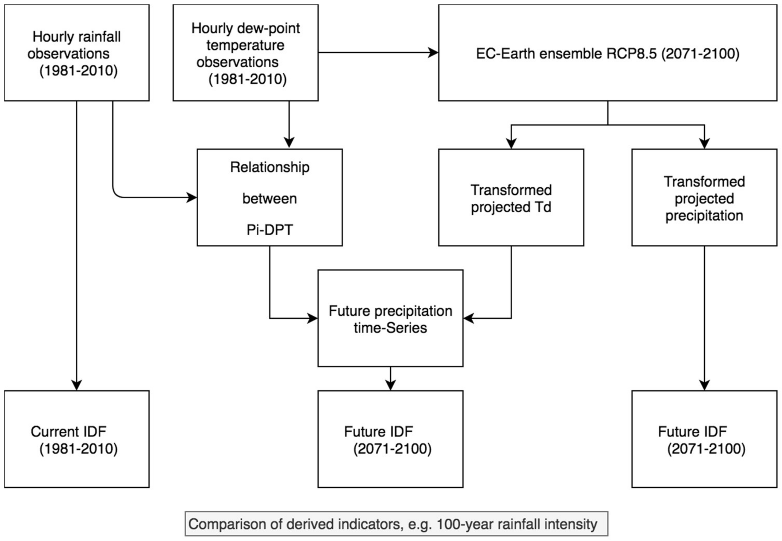
Figure 1 provides an overview of the applied modelling framework and the data that is used. We first present a brief overview after which the individual sections give details of both the data and each analytical step. Observed precipitation and temperature time series data of 33 weather stations in the Netherlands are used to derive the Pi-Td relationship and IDF-curves for the current climate. We use the period of the years 1981–2010 as the baseline. We select a large ensemble of projected climate data from the EC-Earth GCM. Rather than using regional climate model data, we chose GCM data for the case, as these are globally available, and would enable a global application of this method. Regional climate model projection availability is more restricted. Ensemble projections for the Radiative Concentration Pathway (RCP) 8.5 [24] from this GCM are used to derive a future precipitation projection, as well as projected change in dew-point temperature. We select the projections for the years 2071–2100. In the first approach we follow [22] and the precipitation data is bias adjusted following the Advanced Delta Change Method (ADCM), of which the details are explained below. In the second approach, the changes in dew-point temperature in these EC–Earth projections are used to empirically scale future rainfall projection using the historically derived, empirical Pi-Td relationship. We intercompare the future IDF curves that result from these two approaches and analyse the change against the actual IDF based on rainfall observations.
2.1. Climate Data
2.1.1. Current Climate
The observed precipitation intensity (Pi) along with the observed dew-point temperature (Td) are analysed for the Netherlands. For this purpose, hourly meteorological data for Pi and Td are taken from 33 weather stations for the baseline period 1981–2010 from the Royal Netherlands Meteorological Institute (KNMI) (https://www.knmi.nl/nederland-nu/klimatologie/uurgegevens). These 33 stations are located on relatively flat grounds and are closely spaced in a rather homogeneous environment. Therefore, we pool together the data from these stations in order to obtain one dataset equal to a time series of 990 years from which the frequency of rare events can be estimated. This same approach is previously also taken by [18].
2.1.2. Future Climate
The EC–Earth model [25] provides several ensemble simulations for RCP 8.5. We chose this model given that the availability of 16 ensemble simulations provides a more robust estimate of the changes in frequency of rare events, see [26]. Data for the projection period of 2071–2100 is made available by KNMI. These data comprise of gridded data with a cell of size 1.125 by 1.125 degrees over the Netherlands. The simulation for RCP 8.5 scenario represents a high emission scenario [24], and we apply this scenario to analyse a possible high level of change in projected extreme precipitation at the end of the 21st century.
The gridded data for the 16 EC–Earth ensemble runs contain 3-hourly rainfall and dew-point temperature time series for the control period (matching with the baseline period of 1981–2010) and the future scenario (2071–2100). We combine these individual ensemble members and construct one dataset equal to a time series of 480 years. This allows us to better account for natural variability and provides a long enough period to capture the relationship between rare short-duration rainfall events with Td.
2.2. Projection Methods
2.2.1. Advanced Delta Change Method
The simulation of convective type events is not yet possible in GCMs, as convective rainfall is parameterized rather than simulated in GCMs [27]. However, RCM models with convection-permitting resolution (kilometer-scale) are now becoming available [28]. To anticipate changes in extreme precipitation at local scale, both in space and time, from GCM data various downscaling methods can be applied. Dynamic downscaling and statistical downscaling combined with bias correction methods are frequently used to produce climate data at a higher spatial resolution [29]. Both dynamic and statistical downscaling methods, increasing the spatial or temporal resolution from a low-resolution dataset, often are either computationally expensive, depend on the availability of RCMs, or long historical observed time series are needed to create reliable statistical relations. Straightforward bias correction methods are often easier to apply for any location of interest and consist of a generic transformation for adjusting the GCM output. The bias between GCM output and the observed time series for the baseline period is then assumed stationary for the future projection [11]. To provide means of comparison for the Td-Pi scaling approach, we apply a bias correction method: the Advanced Delta Change Method (ADCM). The procedure to apply ADCM is described by Van Pelt et al. [22] and briefly outlined here.
First, the 60th and 90th percentile are calculated for each month. These values are smoothened to reduce the sampling variability of the transformation coefficient a and b. We calculated a weighted mean to smooth: a 0.5 weight is given to the current month and 0.25 weights are given to the previous and next month. The excess (E) is calculated for 3-h precipitations sums which exceeds the 90th percentile of their respective months. The mean control and future period excesses, and , respectively, are calculated on a monthly basis over the entire period using Equation (1). These mean excesses are also smoothened. Second, the correction factors g1 and g2 are calculated, see Equation (2). Then, transformation coefficients a and b are calculated following Equation (3).
Step 1: Calculating the Excess
Step 2: Bias Correction factors
Step 3: Transformation Coefficients
Finally, a transformation of the observed precipitation data is carried out to arrive at the future transformed precipitation series using Equation (4).
Step 4: Transformation
where PO is observed precipitation, PF is future precipitation, PC is control precipitation, P60 is the 60th percentile, P90 is the 90th percentile, E, EC, and EF are the excess for the observed, control, and future periods, and nC and nF are the numbers of values in which the 90th percentile is exceeded in the control and future period.
Using these steps, we calculate the ADCM parameters and coefficients. We transform the precipitation values from the baseline period to the future period using the projected changes in the 60th and 90th percentiles. For this, we aggregate the 1-hourly observed rainfall data to 3-hourly data to align it with the EC-Earth timestep. These data are used in the ADCM and transformed into future precipitation at 3-hourly timestep. This future precipitation is divided by the baseline precipitation to establish the change factor. The baseline hourly precipitation is then multiplied by the change factor for the future precipitation. This results in hourly precipitation time series for the future scenario (2071–2100) for each EC-Earth model ensemble member.
2.2.2. Precipitation Intensity and Dew-Point Temperature Relationship
For the second approach, a relationship is determined between rainfall intensity and dew-point temperatures at hourly intervals. Lenderink et al. [17] found the best relationship between precipitation intensity and dew-point temperature when the Td values 4 h before the observed precipitation are considered. The best relationship here is defined as the most constant dependency across the largest range of dew-point temperatures. After testing several lead times of Td, we confirmed this four-h lead, which is implemented for the rest of the analysis.
For the Pi-Td relationship only wet events are taken into consideration, with Pi > 0. With this wet period time series, Td bins of 1 °C are built across the range of Td. We apply a ceiling approach, Td values between 0 °C and 1 °C are referred to as the Td bin at 1 °C. These bins are then used to group Pi values. For every bin, Pi values corresponding to different percentiles are extracted to create percentile plots. We assessed the 80th and the range of the 90–99th percentile in steps of 1 percentile. Additionally, we assessed the 99–99.9th percentile in steps of 0.1 percentile.
We introduce a conditional operator for calculating the percentile values. The conditional operator ensures that while calculating percentile values within a bin, only those bins are considered which have a minimum number of data points satisfying the particular percentile bin calculation. This reduces uncertainty as for higher percentile values the numbers of precipitation values within a bin reduces. This minimum number of data points is referred to as a threshold value. Once this conditional operator is introduced, it allows us to continue with only those temperature bins which have more precipitation data points than the threshold calculated. With this approach we use a conservative inclusion criterium while simultaneously guaranteeing confidence in the number of data points within in the bins that are included. Equation (5) computes the threshold value for every percentile value. It implies that, e.g., the 99th and the 99.9th percentile at least 100 respectively 1000 data points should be available in the bin to be included in the analysis to establish the Pi-Td relation.
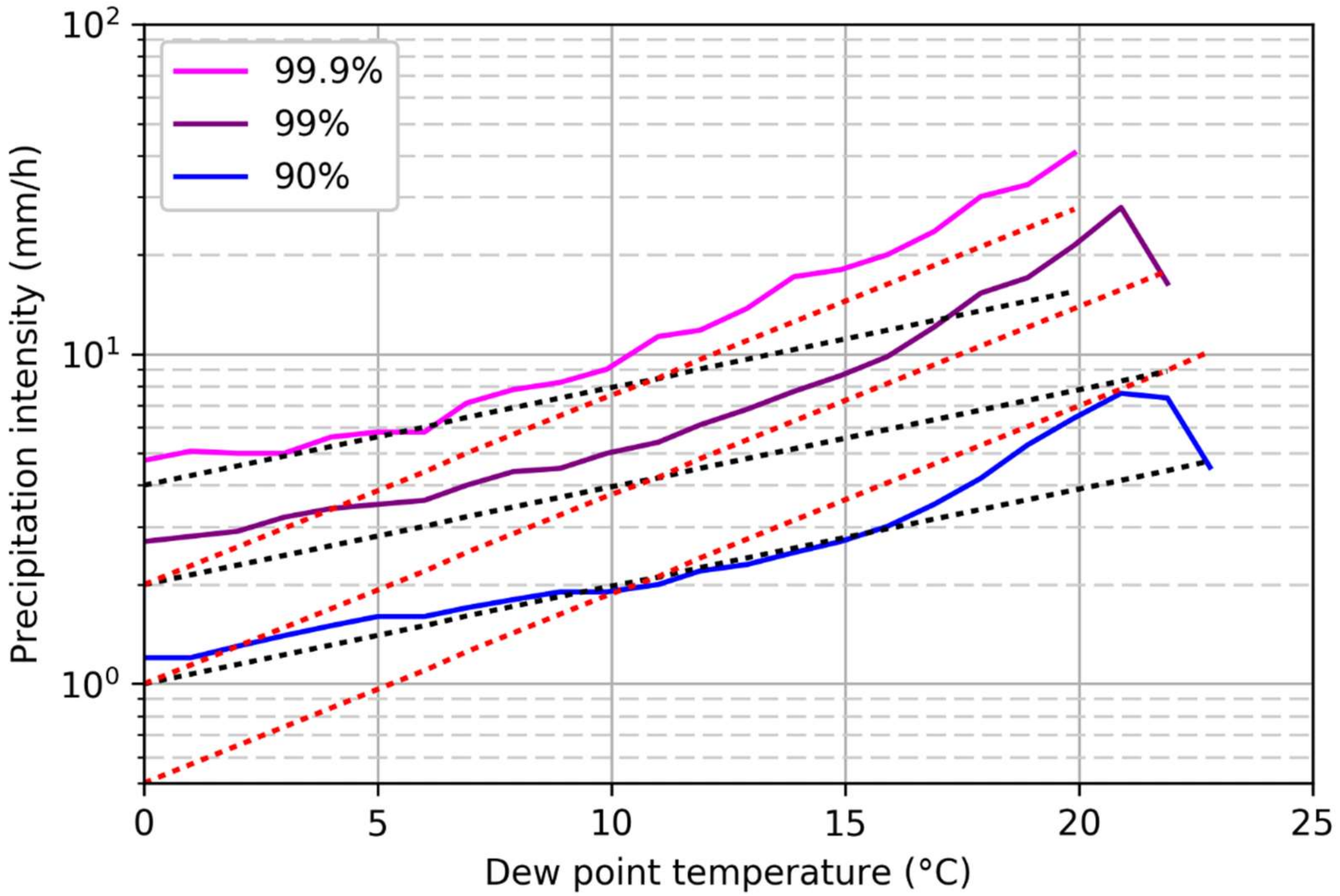
The slope of the Pi-Td relationship generally follows the Clausius–Clapeyron (CC) relationship, with approximately 7% increase in precipitation intensity per 1 °C rise in Td. In case of high percentile values of Pi, the slope of the Pi-Td relationship changes to a slope corresponding to a super Clausius–Clapeyron (sCC) relationship after a certain value of Td, which implies approximately 14% (or more) increase in precipitation intensity per 1 °C rise in Td. This is discussed in more detail in Section 3.1 and can be seen from Figure 2.
We identify the dew-point temperature Td at which the slope of the relationship changes from 7%/1 °C (Clausius–Clapeyron) to about 14%/1 °C (super Clausius–Clapeyron). In addition, we identify the limit of the super Clausius–Clapeyron relationship, i.e., when the 14%/1 °C slope declines.
These two points are identified from multiple percentile plots, between which these values vary. For example, the transition from 7% to 14% occurs at a Td of about 17 °C using the 90th percentile precipitation data but is lower for higher percentiles (between 15 °C and 16 °C). Likewise, the limit of the sCC is found around 21 °C for the 90th percentile precipitation data, however, increases to 23 °C when the 92nd–99th percentile data is analysed. We select as conservative estimates for the transition and limit points the 15 °C and 21 °C temperatures, as these result in the largest increases in rainfall intensities. These points are used in the subsequent analysis, as described in Section 2.2.4.
2.2.3. Temperature Transformation
Similar to the transformation of the GCM precipitation time series, we transformed the GCM dew-point temperature time series representing future climate. Temperature transformation is linear in nature and we follow Shabalova et al. [30] using Equation (6).
We subtract the mean Td value of the baseline period from the mean transformed Td value to calculate the increase in dew-point temperature over the period 1981–2000 to 2071–2100. This increase is hereafter referred as ΔTd.
2.2.4. Dew-Point Temperature Scaling
The empirical relation between dew-point temperature and rainfall intensity [5] can be used to scale rainfall intensity, using projected changes of dew-point temperature (e.g., [14]). The results of the Pi-Td relationships are used to generate precipitation time series for the future scenario (2071–2100) based on the estimated change in Td. We selected a single range of Td where the sCC relationship applies for the different percentiles.
The Piobserved is transformed to the Pifuture using the Pi-Td relationship. The CC relationship adheres to 7% increase in precipitation intensity per 1 °C rise in Td, while the sCC relationship assumes a 14% increase, above an average temperature of Td = 15 °C. This is the integer value of Td of the applied percentile-bins not greater than Td. We apply this floor integer approach as it will include more rainfall events in the sCC domain, hence leading to a conservative projection of the future climate. The average Td at which sCC changes back into CC is established at Td = 21 °C, following the ‘floor integer’ approach. This results in the transformation formula shown in Equation (7).
where α and β represent the Pi-Td change factor and ΔTd the change in dew-point temperature. In this study we apply α = 1.07 for values of Td in the CC domain and beyond the sCC domain. It is expected that the limit of the sCC relation is a statistical artefact, because too few data is available to establish a sCC relation above 21 degrees. But rather than applying a factor of 1.14, we chose to apply a factor of only 1.07, in order not to exaggerate the change in rainfall intensity above Td of 21 degrees. A change factor of β = 1.14 is used for the Td values in the sCC domain. With these two equations we generate a future scenario (2071–2100) for hourly precipitation based on the projected change in Td.
2.3. IDF Curves
We calculate the IDF curves of the observed baseline climate and the future scenario using both ADCM and temperature scaling, resulting in 3 IDF curves. With these the change in rainfall intensity can be assessed, based on the two different methods for projecting changes in future precipitation extremes. IDF curves are constructed for durations of 1-h and 24-h (1 day) for five return periods: 2, 5, 10, 50, and 100-years. We assess the shift in return period of the current rainfall intensities, with a duration of 1-h and 24-h. These durations are relevant for practitioners in local urban planning and water management, and for engineering design purposes of local drainage infrastructure, where hourly or daily precipitation extremes are important.
3. Results
3.1. Observed Pi-Td Relationship
We establish the Pi-Td relationship with the current climate time series. Figure 2 shows these results for the 90th, 99th, and 99.9th percentiles. These results are in line with the work of Lenderink and Van Meijgaard [18]. Pi-Td relationship is clearly dynamic in nature. We find a Pi increase per 1 °C rise in Td ranging from 5%–9%. This is in line with the theoretical CC value of 7% Pi increase per Td rise.
We find that the transition from CC to sCC for the 90th, 99th, and 99.9th percentiles occurs at approximately Td = 17 °C, 16 °C, and 13 °C, respectively. We find that the mean Td value in the 90th-99.9th percentile range at which this CC-sCC transition occurs is at 15 °C. The increase in Pi per Td in this sCC domain is found to be ranging from 15%–23%. This is higher than the generally applied value of 14% for sCC. In the following results we applied the generally excepted 14% Pi increase which can result in a slightly too conservative increase. The 90th and 99th percentiles clearly show a stop to the sCC scaling in the range of 20–23 °C. We find that the mean Td value in the 90th–99.9th percentile range at which this drop occurs is at 21 °C.
3.2. EC-Earth Dew-point Temperature Bias
The parameters derived from the observed climate data and the control and future EC-Earth simulations provide understanding of a possible bias of the EC-Earth model, see Table 1. The bias correction factor g1 shows low values due to a combination of the drizzle effect in GCMs [31] and the 3-h time interval of the time series. The bias correction factor g2 expresses a stronger correction during the April–August period than during the September–March period as the control EC-Earth simulation shows a precipitation depth of, on average, 2.1 times higher than observed at the 90th percentile. The monthly mean daily dew-point temperatures of the control climate are all but during December lower than the observed climate. February and March show considerable percent deviations, while on average the monthly dew-point temperature is only 0.8 °C lower. The standard deviation of the future climate decreases compared to the control climate. Most of the impact is during the November–April period, which sees an average reduction of 12%, equalling 0.5 °C lower. During the May–October period the differences in standard deviation decrease with 3% or 0.1 °C lower. In sum, the bias of the EC-Earth model appears to be minor. In addition, projected changes were calculated using the change only, thereby preserving the projected climate change signal, and removing the bias.
3.3. Future Change in Td
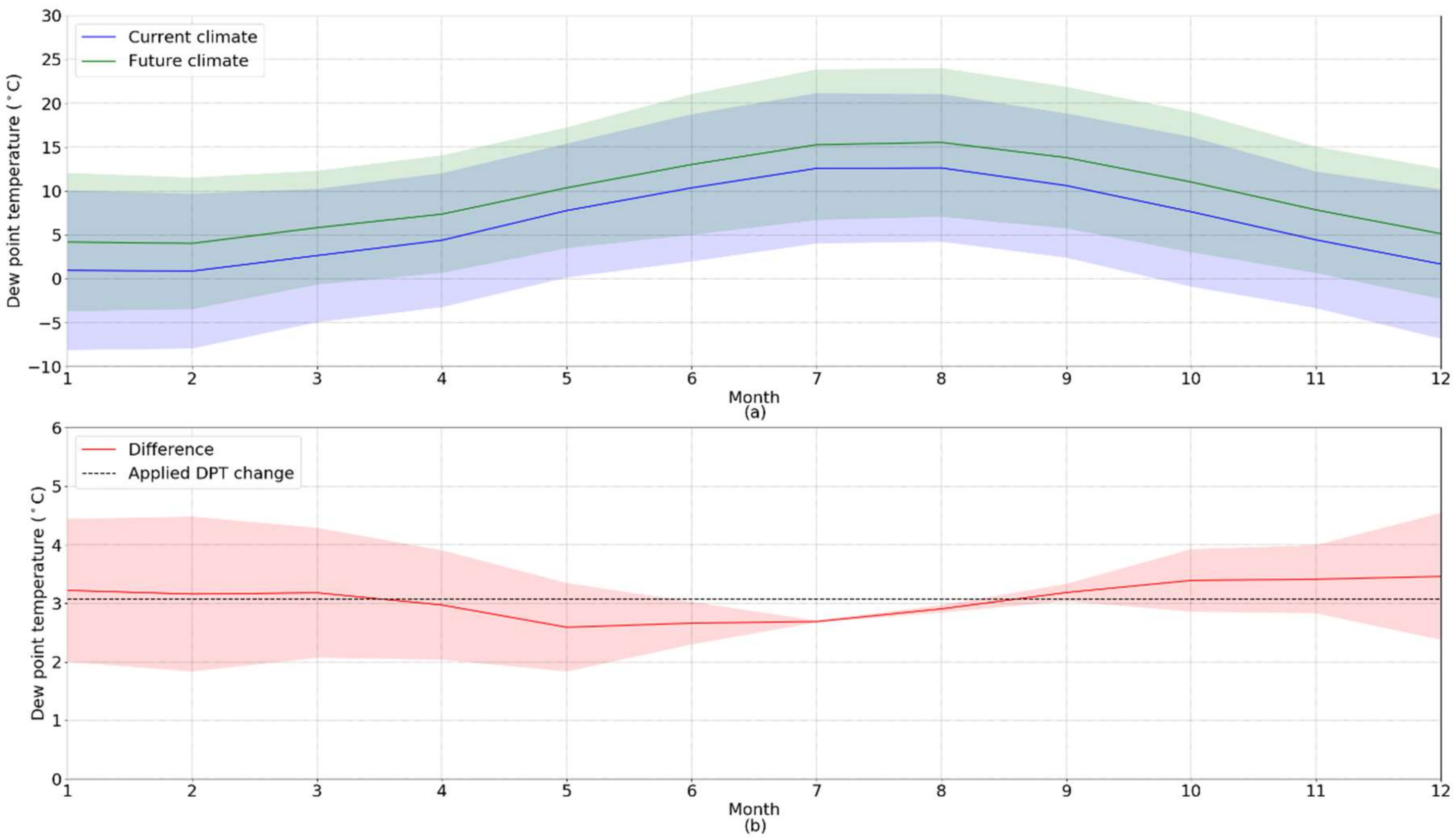
We computed the projected change in dew-point temperature as simulated by the EC-Earth climate model by subtracting the mean Td of the control period (1981–2010) from the mean of the future Td for the period 2071–2100. Figure 3a shows the monthly mean Td values for both current and future climate. Under RCP8.5 the monthly mean Td increases from 2.59 °C in the month of May to 3.46 °C in December, see Figure 3b. It shows a particularly narrow confidence interval for July and August. This could be related to the relatively low air humidity in these months over the Netherlands and thus relatively small variation in dew-point temperature.
The Netherlands experiences most extreme rainfall events with the highest intensities during the summer half year, which runs from May until October. The winter half year (November–April) receives almost an equal amount of cumulative rainfall, but this is often in events with longer duration and low precipitation intensity. The Td is projected to increase by 2.90 °C during the summer half year (May–October). The annual mean Td is projected to increase by 3.07 °C. As this increase is reasonably close to the Td increase during the summer half year, we use this future change in mean Td to calculate future precipitation using Equation (7).
3.4. Comparing the IDF-Curves
We applied Equation (7) using the empirical transition value between CC and sCC of 15 °C and the projected future change in mean Td of 3.07 °C. With these parameter values we scaled the observed Pi time series to establish a future Pi time series. From this time series, we then constructed intensity-duration frequency (IDF) curves.
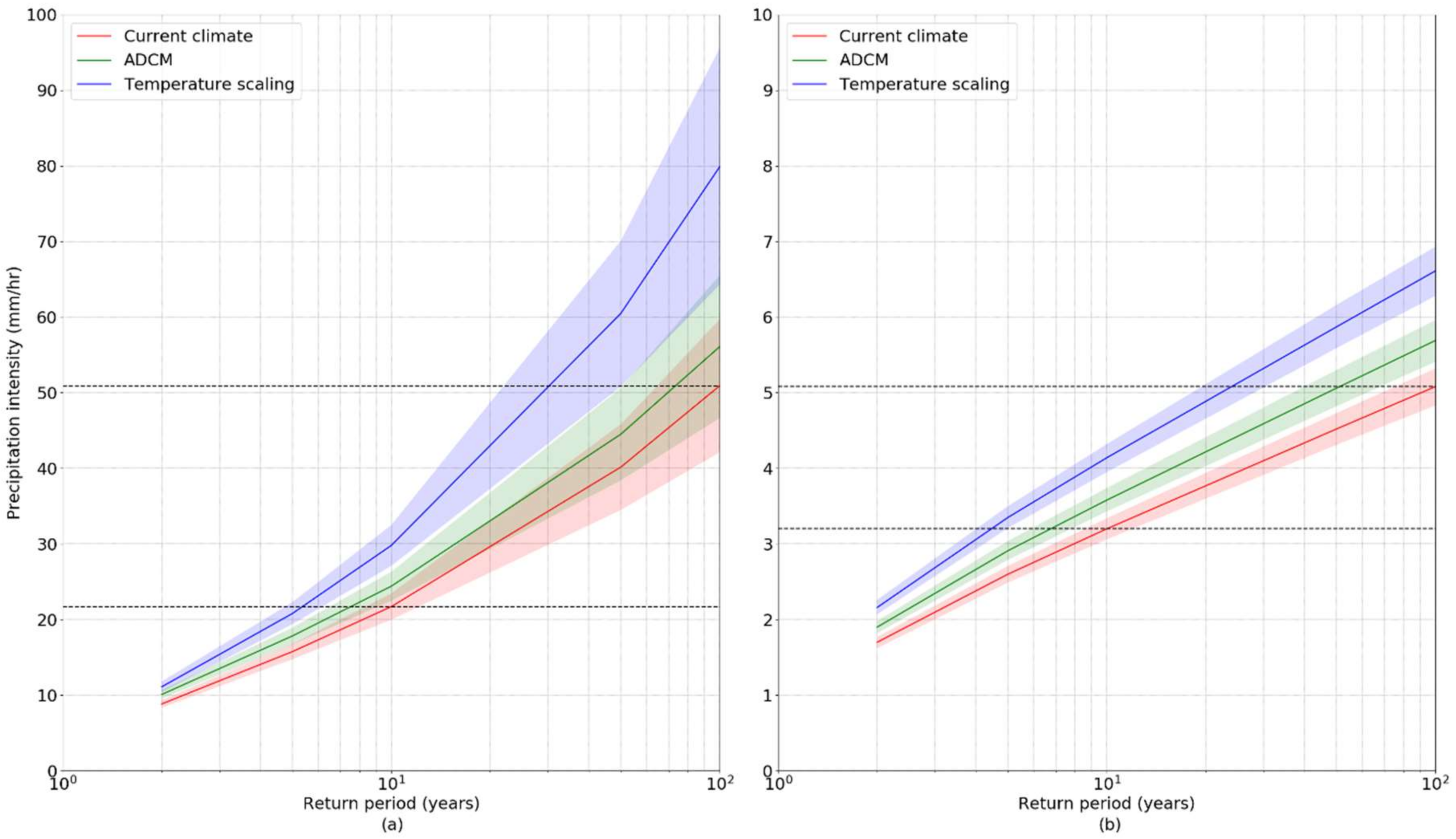
Figure 4a shows the IDFs for a 1-h duration rainfall event for the current climate, as well as a projection for the future climate for RCP 8.5, using the ADCM and dew-point temperature scaling approaches. Figure 4b shows the resulting IDFs for a 24-h duration rainfall event. When focusing on events with a 10-year return period and a 100-year return period we find clear shifts in precipitation intensities.
In the current climate a rainfall event of 21.7 mm within 1-h corresponds with a 10-year return period (range between 8.4–12.1 years, at a 95% confidence level), see Table 2. The estimated return period of a similar precipitation intensity in the future climate in 2071–2100 using the ADCM approach is reduced to 7.5-year (6.5–9.1 years). This rainfall event thus becomes 1.3 times more frequent. We find that using temperature scaling the return period of this event changes to 5.4-year (4.7–6.2 years), which is 1.8 to 2.0 times more frequent than in the current climate. Depending on the scaling method applied, ADCM or temperature scaling, this 21.7 mm 1-h rainfall event occurs 1.3 to 2.0 times more frequent. We find similar patterns with the 1-h duration rainfall event with a 100-year return period. The ADCM scaling results in a 1.3 to 1.4 times more frequent event, and by applying the temperature scaling this becomes 2.9 to 3.8 times more frequent.
The results for a 24-h event show that a 10-year rainfall event, which today has a 3.2 mm/hr precipitation intensity (76.8 mm), will increase in frequency by 1.5 times for future climate following the ADCM scaling. Applying the temperature scaling method results in a 2.1 to 2.4 times more frequent event occurrence. The occurrence of a 100-year event, with a 5.1 mm/h precipitation intensity in current climate (121.8 mm), will become 1.9 to 2.1 times more frequent for the ADCM approach, and 3.9 to 4.6 times more frequent following the temperature scaling approach.
These changes in return periods show that safety standards designed for current climate conditions most likely will not be met without accounting for the additional volume in the future climate. A 1-h event with a 10-year return period will increase 12% to 24.4 mm (22.5–26.3) following the ADCM scaling, and 37% to 29.8 mm (27.1–32.5) with temperature scaling, see Table 3. A similar pattern occurs for the 1-h event with a 100-year return period. The precipitation depth increases 10% and 57%, respectively. The results for a 24-h rainfall event show that the precipitation depth with a 10-year return period will increase 12% following ADCM scaling and 29% following temperature scaling. For events with a 100-year return period the increase in precipitation depth is 12% and 30%, respectively.
To provide a perspective on the importance of applying downscaling and correction methods like ADCM and temperature scaling to raw GCM results, we calculate the precipitation depths using the raw EC-Earth data for the future period. The results for a 24-h rainfall event show that the precipitation depth with a 10-year and a 100-year return period would decrease 54% and 63%, respectively with uncorrected GCM results. This shows how the future changes simulated by the EC-Earth model differ prior to applying valuable and necessary downscaling and correction methods.
4. Discussion
Several choices and limitations apply to the approach presented here. As an important point, we focused on GCM data to explore the potential global application of the temperature scaling method, for any given place around the world. When higher resolution data, e.g., from a RCM, is available that better projects convective rainfall, the procedure could be repeated with such data.
We analysed the sensitivity of the Td values at which CC changes into sCC and the limit Td. The temperature scaling for future precipitation intensity is sensitive to the Td at which CC changes into sCC and the Td at which sCC is limited. If the CC value is applied to a larger domain, i.e., a higher Td value, the changes in future precipitation will decrease. Conversely, should sCC dominate a larger domain, whether due to a lower change Td or a higher limit Td, the changes in future precipitation will increase. In this study we imposed a transition at Td = 15 °C for all percentiles in the Pi-Td relation instead of a percentile dependent transition Td-value which would be more in line with the findings regarding the variable nature of the Pi-Td relation. The current transition may affect the projected changes in rainfall intensities for different percentiles, and therefore at different return periods. Future research could determine a more suitable method to capture the transition from CC into sCC when establishing a Pi-Td relation for scaling future climate. Additionally, we assess the sensitivity of future precipitation to changes in ΔTd by calculating the percentual difference when the limits of the 95% confidence interval would have been applied. For αΔTd, this would result in a −6% to +7% change, while for βΔTd this would lead to a −12% to +14% change in future precipitation.
In this study we apply a β of 1.14 for the sCC domain. However, the observed data show increases in Pi-Td rate in the sCC domain higher than 14%. The actual physical meaning of those values is still subject of research, see, e.g., [32,33], and therefore we apply 14%. Changes in β affect the resulting scaling to establish future precipitation time series. Future research on sCC would help to indicate whether a β of 1.14 remains applicable or whether even higher values could be applied for sub-daily intensities.
One perspective on the impact of more frequent extreme rainfall events is given by the example of the city of Amsterdam. The city expressed the ambition to be able to cope with rainfall events of 60 mm in one hour, by combining drainage and storage in private and public space. The storage in the stormwater system is expected to account for 20 mm and temporary storage in both private and public space for another 40 mm [34]. This corresponds to a return period of about 153 years (100.9–377.1). Following the ADCM approach this 60 mm/h will occur approximately 1.3 times more often. Would the city of Amsterdam follow the temperature-scaling approach, this design event will be 3.1 times more frequent? When the city of Amsterdam would choose to remain at the current safety level, and changes in the corresponding water infrastructure would be built in the coming years, the design should focus on 97.9 mm in one hour. The difference with the current design guideline, 37.9 mm, shows that the effort to create temporary storage should almost double if Amsterdam prefers to maintain their coping capacity with extreme events under RCP 8.5 for 2071–2100.
The comparison between GCM Td scaled precipitation and GCM precipitation is done for the future period of 2071–2100. The RCP 8.5 emission scenario is used, as the interest is to check what could be a high change of rainfall intensity. Using other scenarios, the reported changes in rainfall intensity will likely be lower. Further analysis could compare both approaches, for the period for which observed data is available. In this way, it could be shown which of the two approaches would better estimate the effects of the past ~1.0 °C warming in rainfall extremes. For this purpose, the past 100 years of observations could be split, to estimate effects on the 1:10 year event.
In this study, application of GCM Td precipitation is limited to one case study location only. Therefore, these results might only be applicable for those locations which have similar climate conditions. For further understanding of the GCM Td scaling approach, other locations with different climate conditions could be tested with this approach. The GCM Td precipitation prediction requires high temporal observed data. Therefore, the geographical applicability of the approach is limited to locations where observational data with required temporal resolution is available.
In this study and previous scientific work, the Td approach is introduced, and its value has been demonstrated, we therefore recommend to consider the more extreme projections obtained with the Td approach as well in future design or at least acknowledge the uncertainty that arises from choosing different methods for projecting future climate under climate change. Future meteorological and climate research should confirm the applicability of the Pi-Td relation for projections, and especially the sCC relation, considering the interaction with large-scale atmospheric circulation and changes therein, and thus its actual potential for use in urban flooding assessments.
5. Conclusions
This study demonstrates the utilization of the temperature scaling method and comparison of two different methodologies for predicting future precipitation extremes. Using projections from GCM or RCM data potentially leads to underestimation of the changes in short-duration (sub-daily) rainfall events, because convective precipitation is not yet resolved in such models. Additionally, convection-permitting modelling is not yet available for all locations around the world. Alternative approaches for finding upper-end changes in rainfall are therefore needed in order to develop robust designs. In the absence of RCMs, convection permitting modelling (e.g., [28]), or detailed climate scenarios (e.g., [35]), that have robust information for short duration rainfall, the temperature scaling approach is promising. Research shows the usability of temperature scaling for climate scenario development (e.g., [14,21]). The comparison of the two approaches using IDF curves helps to understand the shift of return period which may occur as the intensity values increase. This explicitly shows that a rare event from a GCM precipitation dataset could be a more frequent event in case a GCM Td scaled precipitation dataset is used.
To project precipitation extremes for the future, the conventional approach of using projected change in short-duration precipitation directly from a GCM may lead to too conservative change estimates compared to the Td scaling approach. For scaling the super Clausius–Clapeyron (sCC) relationship, we considered a fixed slope of 14%. We observed that the sCC slope can also be higher and the use of 14% as fixed slope may still lead to some underestimation of future extremes.
Using the Pi-Td relationship from observational records, it can be explored whether a sCC relation exists for local short-duration rainfall. The Pi-Td based estimated changes in rainfall intensity for 1-h and 24-h durations, for instance, can help drainage engineers and urban planners to adapt their designs.
For an end-user, this implies that in case no information on future changes in convective rainfall extremes is available, besides the rainfall information from a GCM, they could use the output from a Td scaling approach as a second reference. Together, these two projections help to understand what the possible upper limit of precipitation in the future period could be.
Author Contributions
Conceptualization, L.M.B. and R.D.; methodology, A.B., R.D. and F.S.W.; formal analysis, A.B., F.S.W. and R.D.; writing—original draft preparation, R.D., A.B. and L.M.B.; writing—review and editing, L.M.B., R.D., F.S.W., and G.C.; supervision, L.M.B. and G.C.
Funding
This research was supported by the European Commission through the Erasmus Mundus Scholarship programme (A.B.). This research also received funding by the strategic research programs Climate Change and Adaptive Planning and Quantifying Flood Hazards and Impacts of Deltares (R.D., L.M.B., and F.S.W.).
Acknowledgments
We thank Erik van Meijgaard and Geert Lenderink (KNMI) for their suggestions and assistance during the study and for sharing the EC-EARTH ensemble data. We also thank the anonymous reviewers whose comments helped to improve this article.
Conflicts of Interest
The authors declare no conflict of interest.
References
- Notaro, V.; Liuzzo, L.; Freni, G.; La Loggia, G. Uncertainty analysis in the evaluation of extreme rainfall trends and its implications on urban drainage system design. Water 2015, 7, 6931–6945. [Google Scholar] [CrossRef]
- DeGaetano, A.T.; Castellano, C.M. Future projections of extreme precipitation intensity-duration-frequency curves for climate adaptation planning in New York State. Clim. Serv. 2017, 5, 23–35. [Google Scholar] [CrossRef]
- Noor, N.; Ismail, T.; Chung, E.S.; Shahid, S.; Sung, J.H. Uncertainty in rainfall intensity duration frequency curves of peninsular Malaysia under changing climate scenarios. Water 2018, 10, 1750. [Google Scholar] [CrossRef]
- IPCC. Climate Change 2013: The Physical Science Basis. Contribution of Working Group I to the Fifth Assessment Report of the Intergovernmental Panel on Climate Change; Cambridge University Press: Cambridge, UK, 2013. [Google Scholar]
- Lenderink, G.; Van Meijgaard, E. Increase in hourly precipitation extremes beyond expectations from temperature changes. Nat. Geosci. 2008, 1, 511–514. [Google Scholar] [CrossRef]
- Westra, S.; Fowler, H.J.; Evans, J.P.; Alexander, L.V.; Berg, P.; Johnson, F.; Kendon, E.J.; Lenderink, G.; Roberts, N.M. Future changes to the intensity and frequency of short-duration extreme rainfall. Rev. Geophys. 2014, 52, 522–555. [Google Scholar] [CrossRef]
- Fischer, E.M.; Knutti, R. Observed heavy precipitation increase confirms theory and early models. Nat. Clim. Change. 2016, 6, 986–991. [Google Scholar] [CrossRef]
- Prein, A.F.; Gobiet, A. Impacts of uncertainties in European gridded precipitation observations on regional climate analysis. Int. J. Climatol. 2016, 37, 305–327. [Google Scholar] [CrossRef]
- Bao, J.; Sherwood, S.C.; Alexander, L.V.; Evans, J.P. Future increases in extreme precipitation exceed observed scaling rates. Nat. Clim. Chang. 2017, 7, 128. [Google Scholar] [CrossRef]
- Prein, A.F.; Rasmussen, R.M.; Ikeda, K.; Liu, C.; Clark, M.P.; Holland, G.J. The future intensification of hourly precipitation extremes. Nat. Clim. Chang. 2017, 7, 48–52. [Google Scholar] [CrossRef]
- Teutschbein, C.; Seibert, J. Bias correction of regional climate model simulations for hydrological climate-change impact studies: Review and evaluation of different methods. J. Hydrol. 2012, 456–457, 12–29. [Google Scholar] [CrossRef]
- Chen, J.; Brissette, F.P.; Chaumont, D.; Braun, M. Performance and uncertainty evaluation of empirical downscaling methods in quantifying the climate change impacts on hydrology over two North American river basins. J. Hydrol. 2013, 479, 200–214. [Google Scholar] [CrossRef]
- Sørup, H.J.D.; Christensen, O.B.; Arnbjerg-Nielsen, K.; Mikkelsen, P.S. Downscaling future precipitation extremes to urban hydrology scales using a spatio-temporal Neyman-Scott weather generator. Hydrol. Earth Syst. Sci. 2016, 20, 1387–1403. [Google Scholar] [CrossRef]
- Lenderink, G.; Attema, J. A simple scaling approach to produce climate scenarios of local precipitation extremes for the Netherlands. Environ. Res. Lett. 2015, 10, 085001. [Google Scholar] [CrossRef]
- Donnelly, C.; Ernst, K.; Arheimer, B. A comparison of hydrological climate services at different scales by users and scientists. Climate Serv. 2018, 11, 24–35. [Google Scholar] [CrossRef]
- Mattingly, K.S.; Seymour, L.; Miller, P.W. Estimates of Extreme Precipitation Frequency Derived from Spatially Dense Rain Gauge Observations: A Case Study of Two Urban Areas in the Colorado Front Range Region. Ann. Am. Assoc. Geogr. 2017, 107, 1499–1518. [Google Scholar] [CrossRef]
- Lenderink, G.; Mok, H.Y.; Lee, T.C.; van Oldenborgh, G.J. Scaling and trends of hourly precipitation extremes in two different climate zones—Hong Kong and the Netherlands. Hydrol. Earth Syst. Sci. 2011, 15, 3033–3041. [Google Scholar] [CrossRef]
- Lenderink, G.; Van Meijgaard, E. Linking increases in hourly precipitation extremes to atmospheric temperature and moisture changes. Environ. Res. Lett. 2010, 5, 9. [Google Scholar] [CrossRef]
- O’Gorman, P.A. Sensitivity of tropical precipitation extremes to climate change. Nat. Geosci. 2012, 5, 697. [Google Scholar] [CrossRef]
- Bessembinder, J.; Bouwer, L.; Scheele, R. WATCH: Climate and climate change: Protocol for use and generation of statistics on rainfall extremes. Transnational Road Research Programme, Conference of European Directors of Road (CEDR), Brussels. 2018. Available online: http://www.cedr.eu/download/other_public_files/research_programme/call_2015/climate_change/watch/WATCH-Climate-and-climate-change_Protocol-for-use-and-generation-of-statistics-on-rainfall-extremes.pdf (accessed on 4 December 2018).
- Manola, I.; Van den Hurk, B.; De Moel, H.; Aerts, J.C.J.H. Future extreme precipitation intensities based on a historic event. Hydrol. Earth Syst. Sci. 2018, 22, 3777–3788. [Google Scholar] [CrossRef]
- Van Pelt, S.C.; Beersma, J.J.; Buishand, T.A.; Van Den Hurk, B.J.J.M.; Kabat, P. Future changes in extreme precipitation in the rhine basin based on global and regional climate model simulations. Hydrol. Earth Syst. Sci. 2012, 16, 4517–4530. [Google Scholar] [CrossRef]
- Haerter, J.O.; Berg, P. Unexpected rise in extreme precipitation caused by a shift in rain type? Nat. Geosci. 2009, 2, 372–373. [Google Scholar] [CrossRef]
- Van Vuuren, D.P.; Edmonds, J.; Kainuma, M.; Riahi, K.; Thomson, A.; Hibbard, K.; Hurtt, G.C.; Kram, T.; Krey, V.; Lamarque, J.; et al. The representative concentration pathways: An overview. Clim. Chang. 2011, 109, 5–31. [Google Scholar] [CrossRef]
- Hazeleger, W.; Severijns, C.; Semmler, T.; Ştefǎnescu, S.; Yang, S.; Wang, X.; Wyser, K.; Dutra, E.; Baldasano, J.M.; Bintanja, R.; et al. EC-Earth: A seamless Earth-system prediction approach in action. Bull. Am. Meteorol. Soc. 2010, 91, 1357–1363. [Google Scholar] [CrossRef]
- Aalbers, E.E.; Lenderink, G.; van Meijgaard, E.; Van den Hurk, B. Local-scale changes in mean and heavy precipitation in Western Europe, climate change or internal variability? Clim. Dyn. 2018, 50, 4745. [Google Scholar] [CrossRef]
- Arnbjerg-Nielsen, K. Quantification of climate change impacts on extreme precipitation used for design of sewer systems. In Proceedings of the 11the International Conference on Urban Drainage (11ICUD), Edinburgh, Scotland, 31 August–5 September 2008. [Google Scholar]
- Kendon, E.J.; Ban, N.; Roberts, N.M.; Fowler, H.J.; Roberts, M.J.; Chan, S.C.; Evans, J.P.; Fosser, G.; Wilkinson, J.M. Do Convection-Permitting Regional Climate Models Improve Projections of Future Precipitation Change? Bull. Am. Meteorol. Soc. 2017, 98, 79–93. [Google Scholar] [CrossRef]
- Fowler, H.J.; Blenkinsop, S.; Tebaldi, C. Linking climate modeling to impacts studies: recent advances in downscaling techniques for hydrological modeling. Int. J. Climatol. 2007, 27, 1547–1578. [Google Scholar] [CrossRef]
- Shabalova, M.V.; Van Deursen, W.P.A.; Buishand, T.A. Assessing future discharge of the river Rhine using regional climate model integrations and a hydrological model. Clim. Res. 2003, 23, 233–246. [Google Scholar] [CrossRef]
- Dai, A. Precipitation Characteristics in Eighteen Coupled Climate Models. J. Clim. 2006, 19, 4605–4630. [Google Scholar] [CrossRef]
- Loriaux, J.M.; Lenderink, G.; Siebesma, A.P. Large-scale controls on extreme precipitation. J. Clim. 2017, 30, 955–968. [Google Scholar] [CrossRef]
- Schroeer, K.; Kirchengast, G. Sensitivity of extreme precipitation to temperature: the variability of scaling factors from a regional to local perspective. Clim. Dyn. 2018, 50, 3981–3994. [Google Scholar] [CrossRef]
- Waternet. Gemeentelijk Rioleringsplan Amsterdam 2016–2021. Available online: https://www.waternet.nl/siteassets/ons-water/gemeentelijk-rioleringsplan-amsterdam-2016-2021.pdf (accessed on 4 December 2018). (In Dutch).
- KNMI. KNMI’14 Climate Scenario’s for the Netherlands. 2015. Available online: http://www.climatescenarios.nl/images/Brochure_KNMI14_EN_2015.pdf (accessed on 4 December 2018).
Figure 1.
Approach for intensity-duration-frequency (IDF) construction including temperature scaling to derive future short-term precipitation extremes.
Figure 1.
Approach for intensity-duration-frequency (IDF) construction including temperature scaling to derive future short-term precipitation extremes.

Figure 2.
Pi-Td relationship for different percentile values (solid lines). The black dotted line indicates the Clausius–Clapeyron (CC) relationship (+7% Pi/Td) and the red dotted line shows the super Clausius-Clapeyron (sCC) relation (+14% Pi/Td).
Figure 2.
Pi-Td relationship for different percentile values (solid lines). The black dotted line indicates the Clausius–Clapeyron (CC) relationship (+7% Pi/Td) and the red dotted line shows the super Clausius-Clapeyron (sCC) relation (+14% Pi/Td).

Figure 3.
(a) Current and future monthly mean dew-point temperatures with 95% confidence intervals, and (b) monthly averaged increase in dew-point temperature under RCP8.5 with 95% confidence intervals. The black dotted line shows the increase in Td as used.
Figure 3.
(a) Current and future monthly mean dew-point temperatures with 95% confidence intervals, and (b) monthly averaged increase in dew-point temperature under RCP8.5 with 95% confidence intervals. The black dotted line shows the increase in Td as used.

Figure 4.
Intensity-duration-frequency (IDF) curves for current climate and future climate projected following Advanced Delta Change Method (ADCM) and the temperature scaling (a) 1-h events, and (b) 24-h events with 95% confidence interval indicated. The dashed lines represent the 10-year and 100-year precipitation intensities for the current climate.


Table 1.
Monthly parameter values for the observed, control, and future climate.
| Month | g1 (-) | g2 (-) | σC (°C) | σF (°C) | |||
|---|---|---|---|---|---|---|---|
| 1 | 4.6E-12 | 0.78 | 4.2 | 3.6 | 1.0 | 0.9 | 4.1 |
| 2 | 5.1E-12 | 0.78 | 4.3 | 3.7 | 0.9 | 0.1 | 3.3 |
| 3 | 5.8E-12 | 0.70 | 4.2 | 3.6 | 2.7 | 1.0 | 4.2 |
| 4 | 5.5E-12 | 0.50 | 3.9 | 3.4 | 4.4 | 3.7 | 6.7 |
| 5 | 5.1E-12 | 0.43 | 3.5 | 3.1 | 7.8 | 6.8 | 9.3 |
| 6 | 5.3E-12 | 0.46 | 3.0 | 2.8 | 10.4 | 9.5 | 12.1 |
| 7 | 5.4E-12 | 0.47 | 2.6 | 2.6 | 12.6 | 11.4 | 14.1 |
| 8 | 4.8E-12 | 0.53 | 2.6 | 2.6 | 12.6 | 11.4 | 14.3 |
| 9 | 4.7E-12 | 0.69 | 2.9 | 2.8 | 10.6 | 9.8 | 13.0 |
| 10 | 5.0E-12 | 0.88 | 3.3 | 3.1 | 7.6 | 7.1 | 10.5 |
| 11 | 5.1E-12 | 0.93 | 3.6 | 3.3 | 4.4 | 4.1 | 7.5 |
| 12 | 4.8E-12 | 0.85 | 3.9 | 3.5 | 1.7 | 1.9 | 5.4 |
Table 2.
Change in 10-year and 100-year return periods for future climate.
| Event Duration (h) | Precipitation Intensity (mm/h) | Current Climate (Return Period in Years) | ADCM Approach (Return Period in Years) | Temperature Approach (Return Period in Years) |
|---|---|---|---|---|
| 1 | 21.7 | 10 (8.4–12.1) | 7.5 (6.5–9.1) | 5.4 (4.7–6.2) |
| 50.9 | 100 (64.5–192.2) | 73.4 (50.7–134.3) | 30.3 (22.0–50.3) | |
| 24 | 3.2 | 10 (8.6–12.0) | 6.7 (5.9–7.8) | 4.5 (4.0–5.0) |
| 5.1 | 100 (75.0–138.0) | 50.8 (39.7–67.2) | 23.9 (19.4–30.2) |
Table 3.
Change in 10-year and 100-year precipitations depths for future climate.
| Event Duration (h) | Return Period (Years) | Precipitation Depth Current Climate (mm) | Precipitation Depth ADCM Approach (mm) | Precipitation Depth Temperature Approach (mm) |
|---|---|---|---|---|
| 1 | 10 | 21.7 (20.0–23.5) | 24.4 (22.5–26.3) | 29.8 (27.1–32.5) |
| 100 | 50.9 (42.1–59.7) | 56.1 (46.7–65.5) | 79.9 (64.3–95.6) | |
| 24 | 10 | 76.8 (73.4–80.2) | 86.0 (82.3–89.8) | 99.4 (94.8–103.7) |
| 100 | 121.8 (116–127.7) | 136.5 (129.9–143.0) | 158.6 (150.7–166.3) |
© 2019 by the authors. Licensee MDPI, Basel, Switzerland. This article is an open access article distributed under the terms and conditions of the Creative Commons Attribution (CC BY) license (http://creativecommons.org/licenses/by/4.0/).
Share and Cite
MDPI and ACS Style
Dahm, R.; Bhardwaj, A.; Sperna Weiland, F.; Corzo, G.; Bouwer, L.M. A Temperature-Scaling Approach for Projecting Changes in Short Duration Rainfall Extremes from GCM Data. Water 2019, 11, 313. https://doi.org/10.3390/w11020313
AMA Style
Dahm R, Bhardwaj A, Sperna Weiland F, Corzo G, Bouwer LM. A Temperature-Scaling Approach for Projecting Changes in Short Duration Rainfall Extremes from GCM Data. Water. 2019; 11(2):313. https://doi.org/10.3390/w11020313
Chicago/Turabian StyleDahm, Ruben, Aashish Bhardwaj, Frederiek Sperna Weiland, Gerald Corzo, and Laurens M. Bouwer. 2019. "A Temperature-Scaling Approach for Projecting Changes in Short Duration Rainfall Extremes from GCM Data" Water 11, no. 2: 313. https://doi.org/10.3390/w11020313
Note that from the first issue of 2016, this journal uses article numbers instead of page numbers. See further details here.