Calculation of Joint Return Period for Connected Edge Data
by
 , , ,
, , ,
Guilin Liu
1, 
Baiyu Chen
2,*,
Zhikang Gao
1,
Hanliang Fu
3,
Song Jiang
3,
Liping Wang
4 and
Kou Yi
5 1
College of Engineering, Ocean University of China, Qingdao 266100, China
2
College of Engineering, University of California Berkeley, Berkeley, CA 94720, USA
3
School of Management, Xi’an University of Architecture and Technology, Xi’an 710055, China
4
School of Mathematical Sciences, Ocean University of China, Qingdao 266100, China
5
Molecular and Computational Biology, University of Southern California, Los Angeles, CA 90089, USA
*
Author to whom correspondence should be addressed.
Water 2019, 11(2), 300; https://doi.org/10.3390/w11020300
Submission received: 11 December 2018
/
Revised: 31 January 2019
/
Accepted: 1 February 2019
/
Published: 11 February 2019
(This article belongs to the Section Hydraulics and Hydrodynamics)
Abstract
:For better displaying the statistical properties of measured data, it is particularly important to select a suitable multivariate joint distribution model in ocean engineering. According to the characteristics and properties of Copula functions and the correlation analysis of measured data, the nonlinear relationship between random variables can be captured. Additionally, the models based on the Copula theory have more general applicability. A series of correlation measure index, derived from Copula functions, can expand the correlation measure range among variables. In this paper, by means of the correlation analysis between the annual extreme wave height and the corresponding wind speed, their joint distribution models were studied. The newly established two-dimensional joint distribution functions of the extreme wave height and the corresponding wind speed were compared with the existing two-dimensional joint distributions.
1. Introduction
Coastal and ocean engineering is generally under the influence of extreme wind wave, which has a high risk of damage. Extreme ocean waves belong to multidimensional random variable that is of interdependence. In recent years, with the requirement of ocean engineering structure reliability and the environmental design standard improving, extreme value distributions of single variables can no longer meet the need of researchers [1,2,3,4]. Researchers pay more and more attention to the theory of multivariate distribution [5,6,7], such as the joint distributions of wave heights, wave periods, and corresponding wind speeds [8,9]. Actually, the damage of coastal and ocean engineering are usually the result of their combined effect. Currently, the theory of multivariate distribution has been applied in many fields [10,11,12,13,14,15,16]. Many application examples have also shown that the design parameters derived from a joint probability distribution can better meet the design need of ocean engineering [17,18,19,20], reduce the building cost of ocean engineering more reasonably, explore return periods of multivariable waves, and calculate joint design level values more accurately. Additionally, all of these are of great significance for the design and risk management of related projects [21].
Currently, the commonly used two-dimensional joint distribution models are the mixed Gumbel, bivariate Logistic, Gumbel-Logistic, and two-dimensional Pearson joint distributions. Yue [22] used the mixed Gumbel distribution to analyze the rainstorm frequency; Zhou and Duan [23] used Gumbel-Logistic model to analyze the joint distribution of extreme wind speed and significant wave height; Dong et al. [24] used the two-dimensional Pearson joint distribution to analyze the joint design parameter estimation of annual extreme winds and waves. However, it is usually necessary to meet certain constraints when using these traditional joint distributions. That is, the marginal distribution model should be the same as the marginal distribution model of the traditional joint distribution [25,26,27,28,29]. For example, the mixed Gumbel distribution requires the marginal distribution to be Gumbel distribution. In order to solve this limitation, Copula function has gradually become the focus of researchers. The Copula function describing multivariate correlation structure promotes the application of multivariate joint distribution and its risk probability in coastal and ocean engineering. Additionally, the Copula function was first proposed by Sklar [30] in 1959, and it has been applied in many fields [31,32,33,34]. The Copula function used in constructing the two two-dimensional joint distribution is able to describe both the non-normality of a single factor (such as wave height, wind speed, water level, etc.), and the complex relationship between different wave elements. For example, the joint distribution of wind speed and wave height or wave height and period can be constructed by Archimedes Copula function that describes the joint distribution of two variables. Currently, the concept of Copula has been abstracted into theory [35,36,37,38]. The Copula function can connect multiple ocean wave elements with non-normal properties and correlation, thus constructing a joint distribution of multiple ocean wave elements. The two-dimensional joint distribution constructed by the Copula function has no strict requirements on the form of the marginal distribution. For this reason, it is more suitable for practical applications.
This paper will analyze the correlation between the annual extreme wave height and the corresponding wind speed by an engineering example, and study the joint distribution models of the two. Then, we will select Gumbel-Hougaard (GH) Copula function and Clayton Copula function, suitable for describing the annual extreme wave height and the corresponding wind speed, to establish two-dimensional joint distribution functions of the extreme wave height and the corresponding wind speed. The established distributions will be compared with the mixed Gumbel distribution and Gumbel-Logistic distribution. Finally, the joint return period analysis and conditional probability analysis of annual extreme wave height and wind speed will be carried out.
2. Common Copula Functions and Distribution Characteristics
Copula theory was first proposed by Sklar in 1959 when the relationship between low dimensional marginal distribution numbers, low dimensional marginal distribution function, and multi-dimensional joint distribution function was studied. With the concept of Copula put forward and its theory gradually improved, Nelsen [39] made a strict definition of Copula in 1999, and presented the Sklar theorem that is important in the application of Copula theory. The Sklar theorem stated that if F(x,y) is the joint distribution function of the random vector (X, Y), and Fx(x) and Fy(y) are corresponding marginal distributions, there must be a correlation structure function C that enables Equation (1) true.
Additionally, when the marginal distributions are continuous distribution functions, C is unique.
Gumbel-Hougaard (GH) Copula function and Clayton Copula function are two Copula functions suitable for describing the positive correlation between variables, which are widely used in the fields of ocean engineering and hydrometeorology. Its distribution function and density function are as follows:
First, the Gumbel-Hougaard (GH) Copula function:
where u and v are corresponding marginal distributions, θ is the parameter of Copula function.
The corresponding density function is:
Gumbel-Hougaard (GH) Copula is only suitable for the condition in which variables are of positive correlation, and mainly describes the upper tail correlation between random variables.
Second, the Clayton Copula function:
The corresponding density function is:
Like the Gumbel-Hougaard (GH) Copula function, the Clayton Copula function is only suitable for the condition in which variables are of positive correlation, and mainly describes the lower tail correlation between random variables in the joint distribution. In addition to the above two two-dimensional Copula functions, the other two common Copula functions are as follows:
Third, Ali-Mikhail-Haq (AMH) Copula function:
The AMH function can describe the random variables with positive or negative correlation, but it is not suitable for the variables with high positive or negative correlation. AMH Copula structure is symmetrical.
Fourth, the Frank Copula function:
It is similar to AMH Copula function, but has no restriction on the degree of correlation. Frank Copula structure is of symmetry, that is, the correlation between the variables increases symmetrically at the upper tail and lower tail of its distribution.
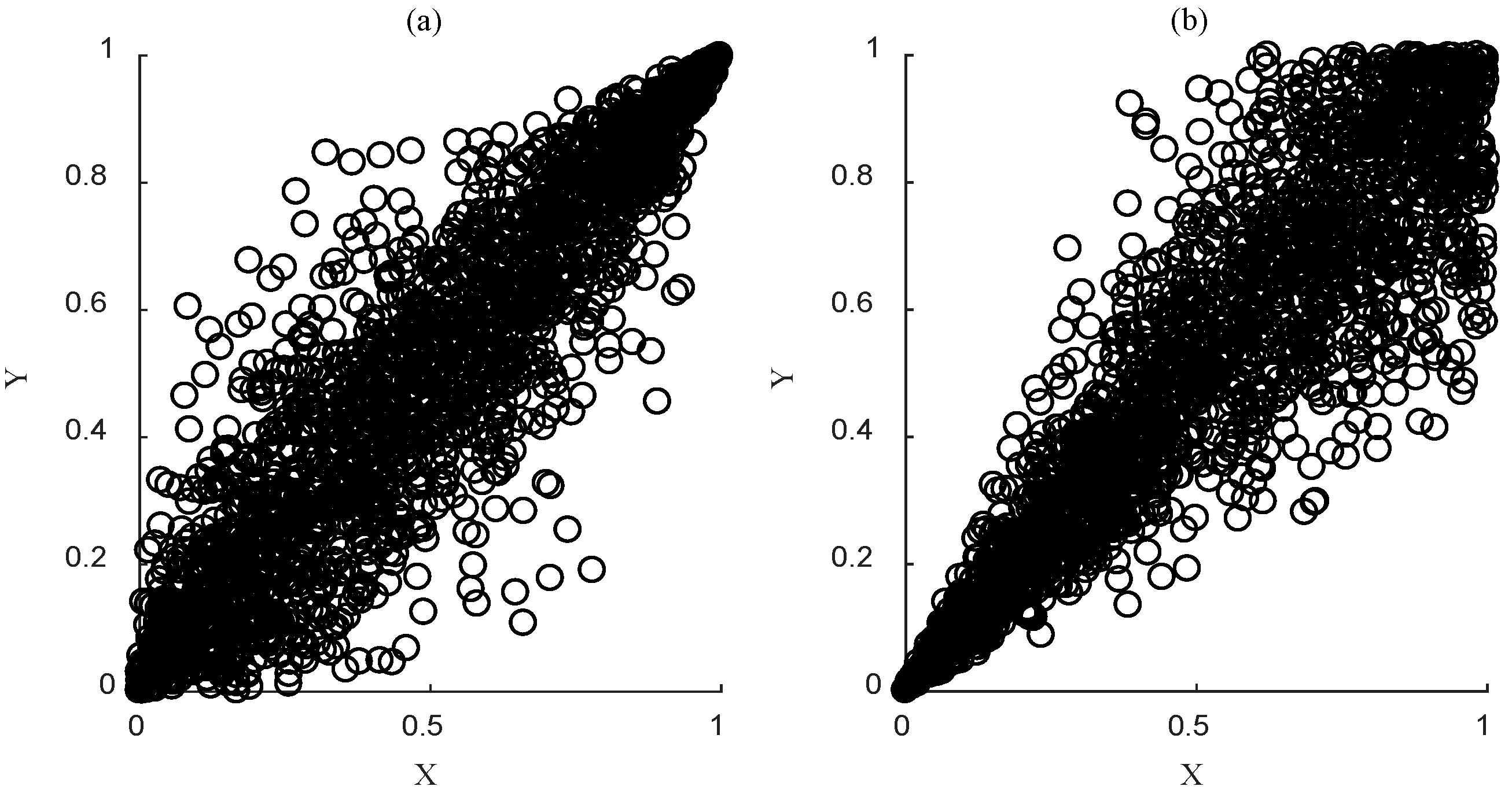
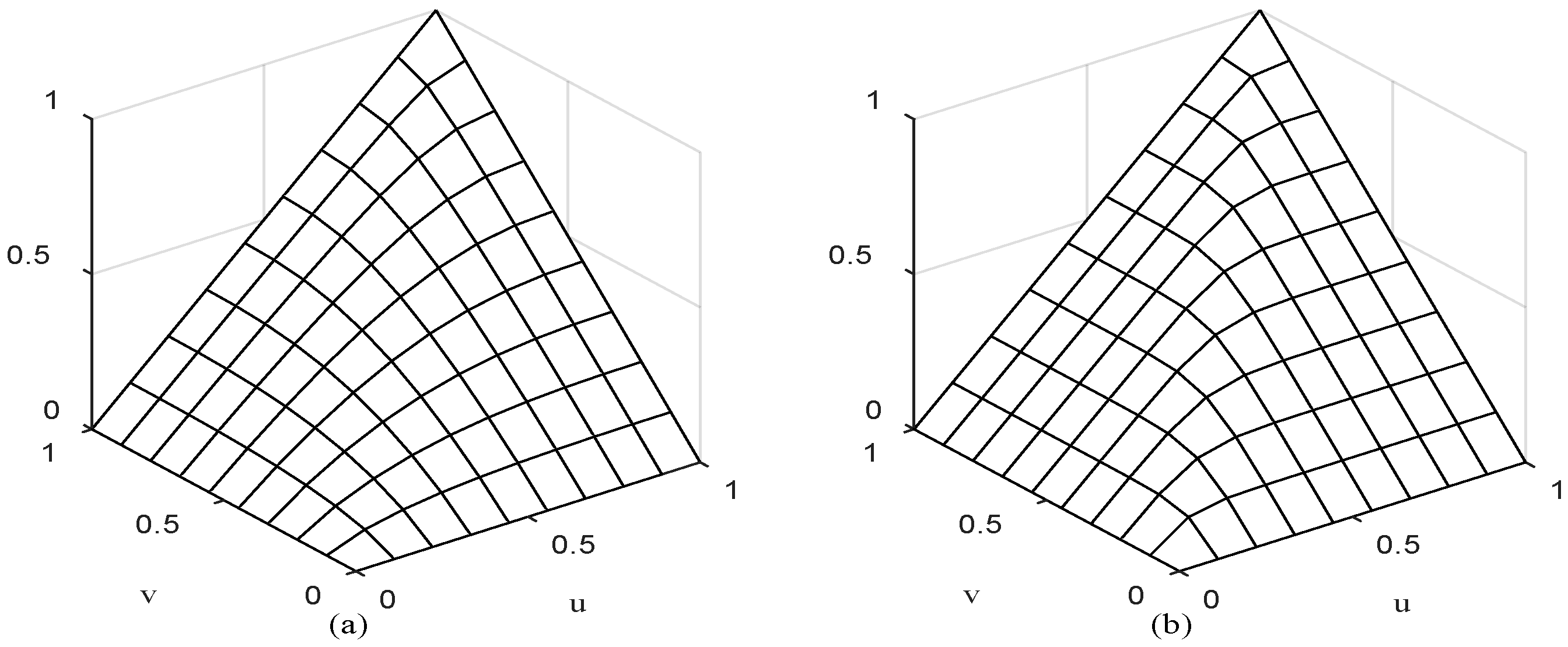
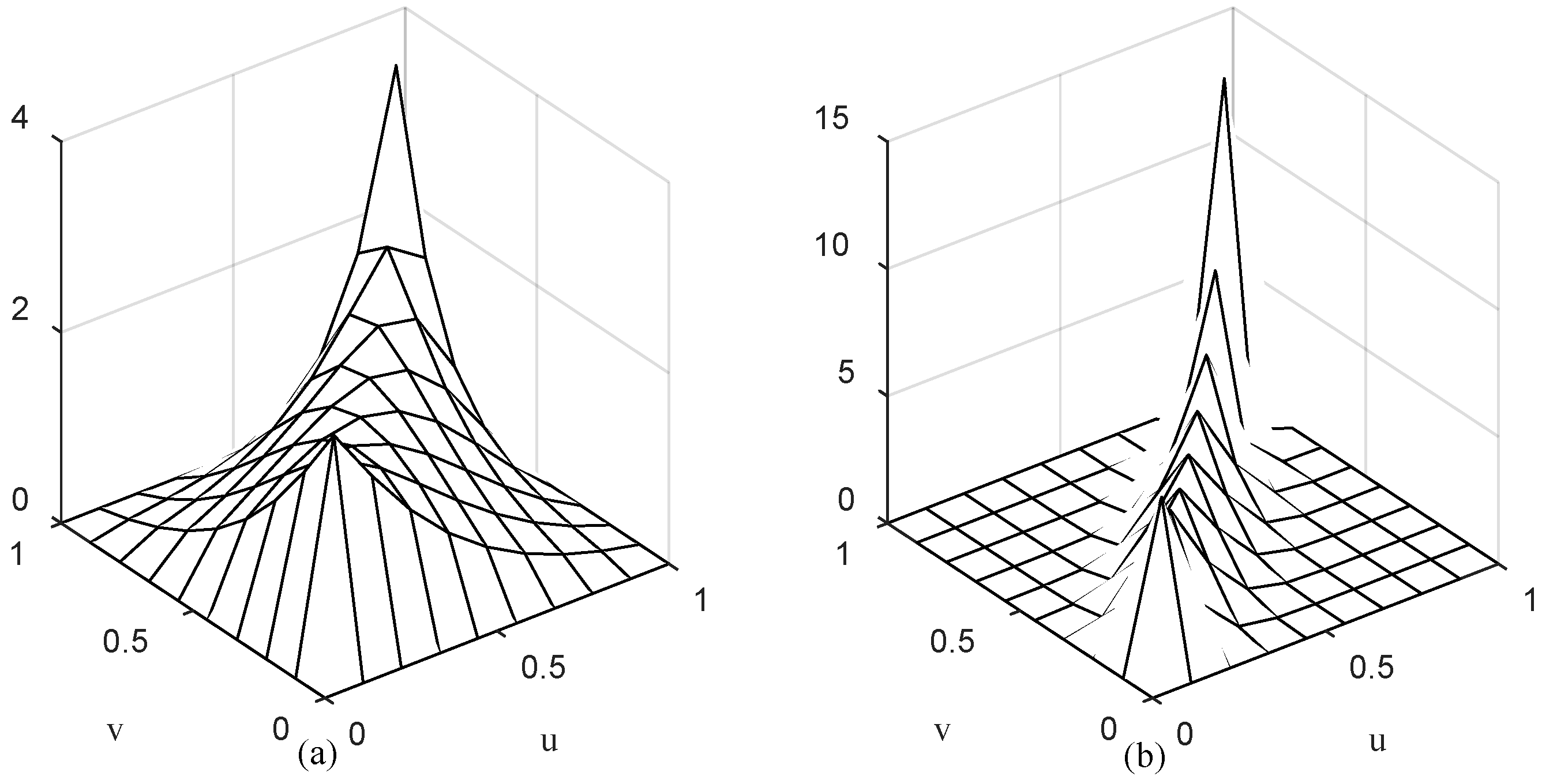
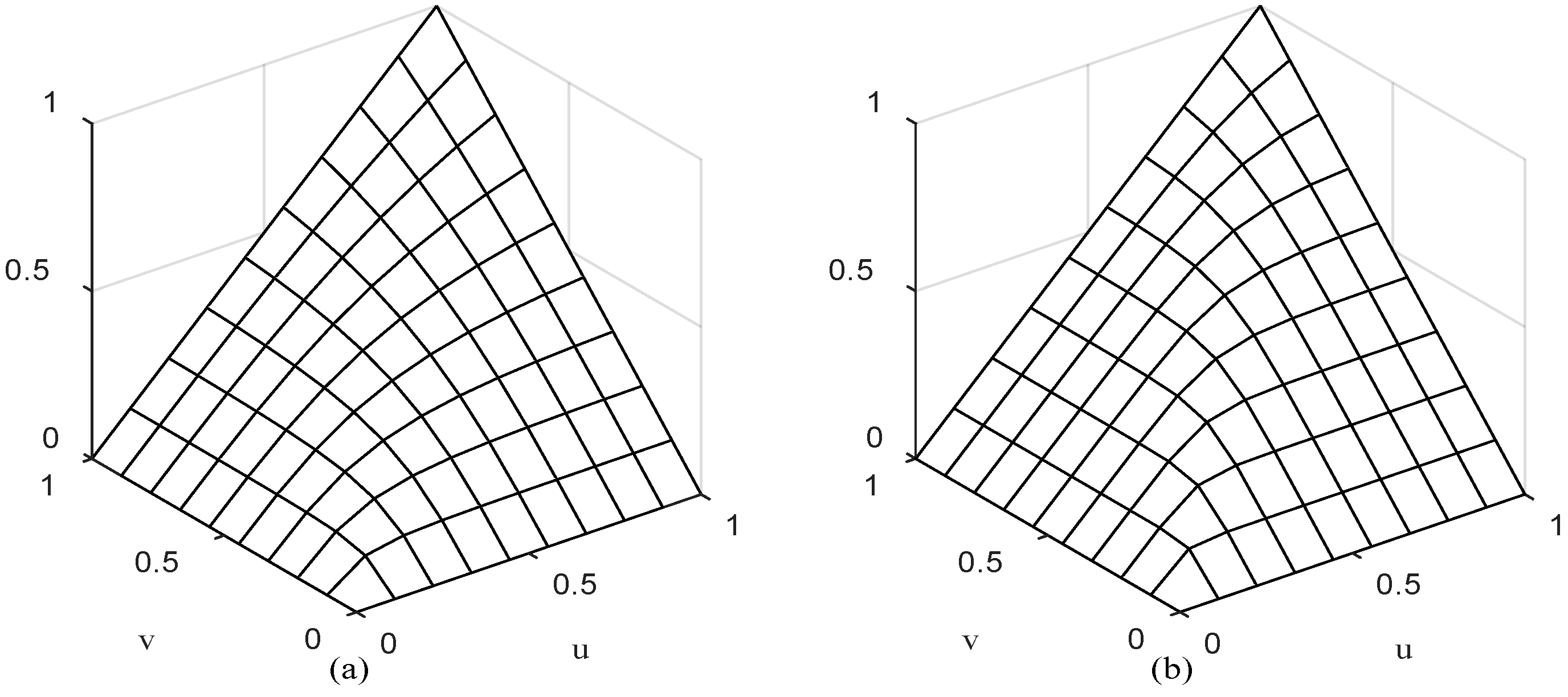
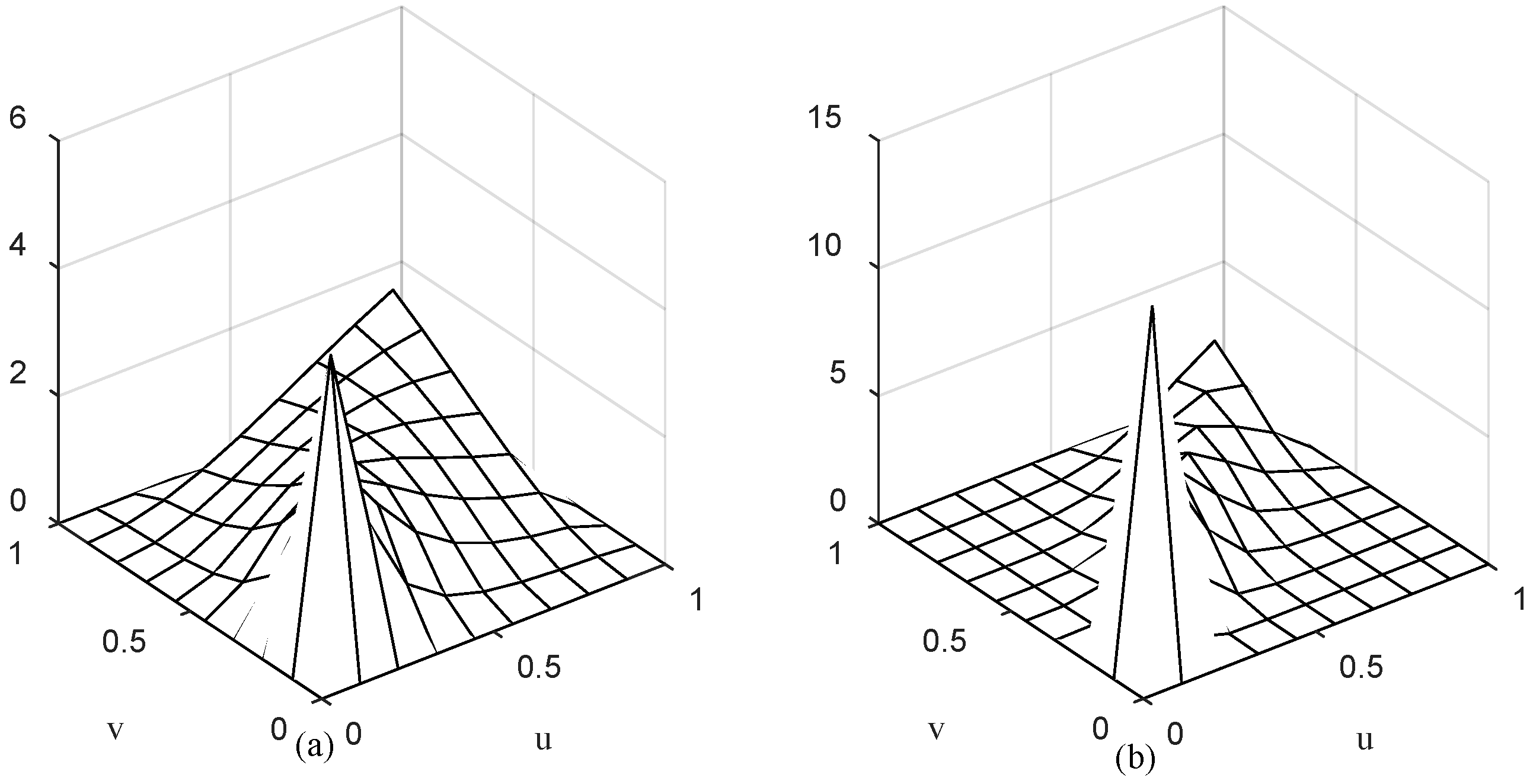
In order to understand Copula functions intuitively, the diagrams of scatter, functions and probability functions are used to describe the distribution characteristics of the above two Copula functions. Figure 1a,b are the scatter diagrams of the Gumbel-Hougaard (GH) Copula function and the Clayton Copula function after 2000 times of stochastic simulation (the value of parameter θ is 4 for GH Copula function, and 6 for Clayton Copula function), respectively. Figure 2a,b are the diagrams of the Gumbel-Hougaard (GH) Copula function when θ is two and four, respectively. Figure 3a,b are the diagrams of the Gumbel-Hougaard (GH) Copula density function when θ is two and four, respectively. Figure 4a,b are the diagrams of the Clayton Copula function when θ is two and four, respectively. Figure 5a,b are the diagrams of the Clayton Copula density function when θ is two and four, respectively.
As shown in Figure 1, after 2000 times of stochastic simulation, the Gumbel-Hougaard (GH) Copula function shows more obvious tendency of a fat upper tail, while Clayton Copula function is more intensive in the lower tail, and scattered in the upper tail. The similar characteristics can be seen from Figure 3 and Figure 5. When θ is two and four, the Gumbel-Hougaard (GH) Copula density function appears as a J-shaped distribution, namely, the upper tail is higher than the lower tail. Thus, Gumbel-Hougaard (GH) Copula function is very sensitive to the correlation of the upper tail among variables. For Clayton Copula function, the tail behavior is quite the opposite. When θ is two and four, Clayton Copula density function tends towards an L-shaped distribution. That is, the lower tail is higher than the upper tail, and the Copula function is very sensitive to the correlation of the lower tail among variables.
3. Examples of the Application of the Copula Function
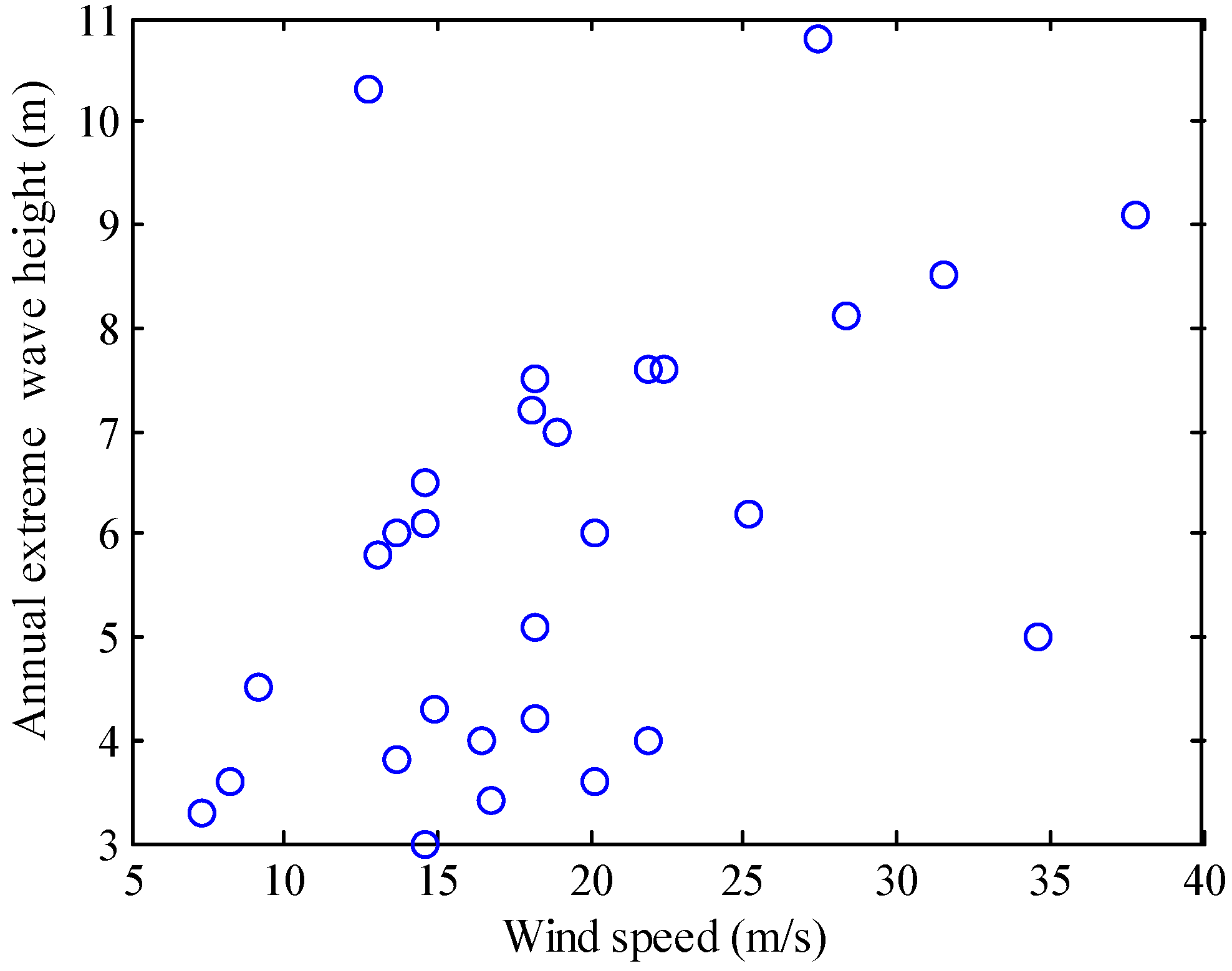
Taking the time series of the annual extreme wave height and corresponding wind speed measured at the Weizhou Island Ocean Station as an example, this paper discussed the validity of two-dimensional joint distribution constructed by Copula functions, when used in ocean engineering. Weizhou Island Ocean station (196°20′ E, 10°90′ N) is located in the South China Sea area. We used the data of the annual extreme wave heights and corresponding wind speeds during 1970–1990 as an example. Its linear correlation coefficient ρ and rank correlation coefficient τ are shown in Table 1.
Table 1 shows the linear correlation coefficient of the data is 0.4992 and the rank correlation coefficient is 0.383. The linear correlation coefficient is well known, and can be expressed as,
where xi stands for the ith observation value of X and is the mean value of X; yi stands for the ith observation value of Y and is the mean value of Y.
It reflects the linear correlation between two random variables X and Y. The rank correlation coefficient is also called the relational coefficient of gradation, and its expression is:
where di is the corresponding rank difference and n represents the number of the data in the dataset. The rank correlation coefficient reflects the correlation between the annual extreme wave height and corresponding wind speed. Figure 6 is a scatter plot of wind speed and annual extreme wave height. The scatter plot of the two is shown below:
Table 1 presents the correlation coefficient analysis, and results there is positive correlation between the annual extreme wave height and wind speed. Therefore, it is reasonable to use the Gumbel-Hougaard Copula function and Clayton Copula function to construct the two-dimensional joint distribution of annual extreme wave height and wind speed. As for the parameter estimation of the Copula function, the most common and concise method is the rank correlation coefficient. The rank correlation coefficient and the parameters meets:
The parameters of the above two Copula functions are easily calculated as 1.6207 and 1.2415, respectively, through the rank correlation coefficient shown in Table 1.
To construct the two-dimensional joint distribution by Copula function, the marginal distribution need to be determined, namely, the single variable extreme distributions of annual extreme wave height and wind speed are in need of determination, respectively. The two-dimensional mixed Gumbel distribution was first proposed by Gumbel, and the Gumbel density function and distribution function of its marginal distribution are:
where x stands for the observation value, σ and μ are two undetermined parameters, f(x; μ, σ) is the Gumbel density function and F(x; μ, σ) is the Gumbel distribution function.
Two-dimensional mixed Gumbel joint probability density function (PDF) and distribution function (CDF) are expressed as follows:
where
and ρ is linear correlation coefficient:
where c, d, σ1 and σ2 are four undetermined parameters, g(x, y) is two-dimensional mixed Gumbel joint probability density function and G(x, y) is the corresponding distribution function.
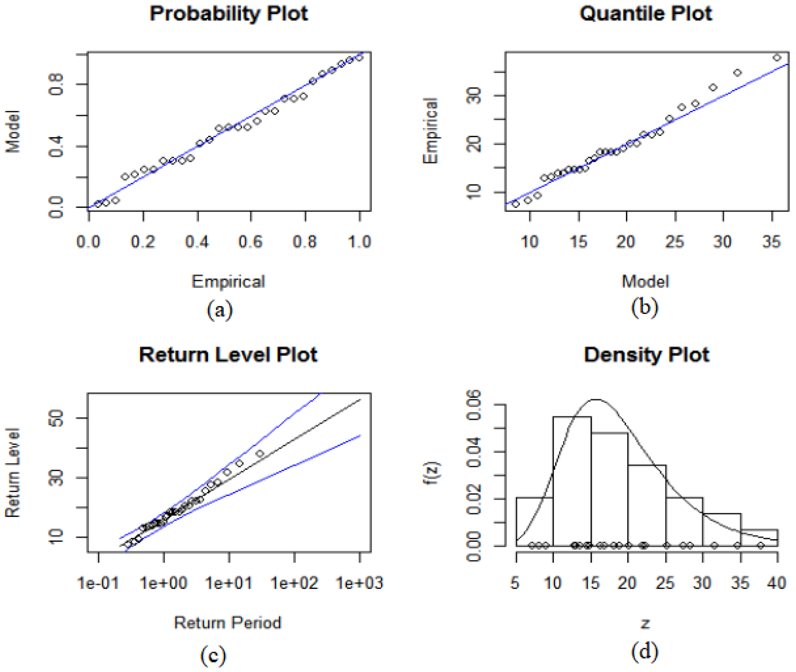
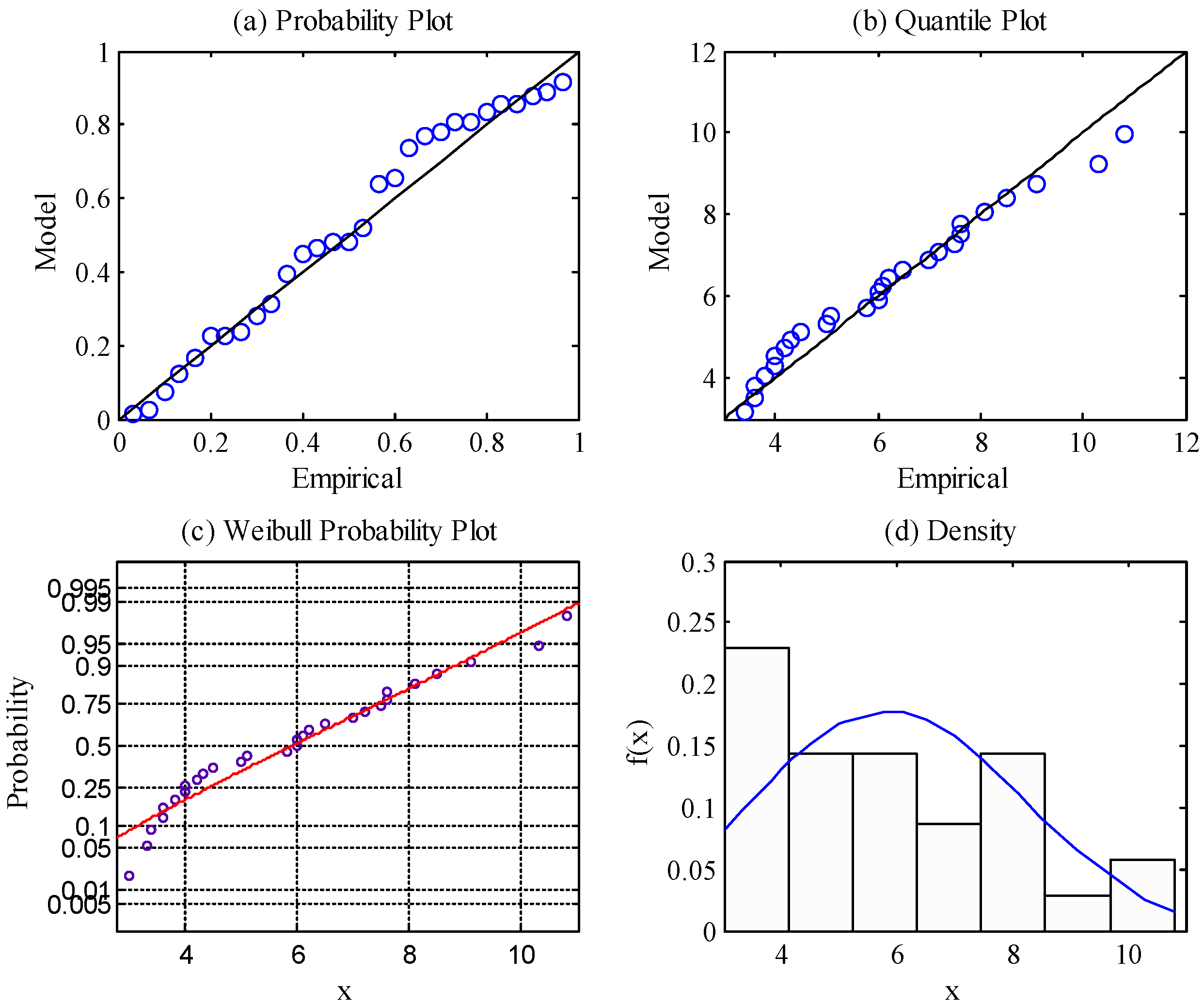
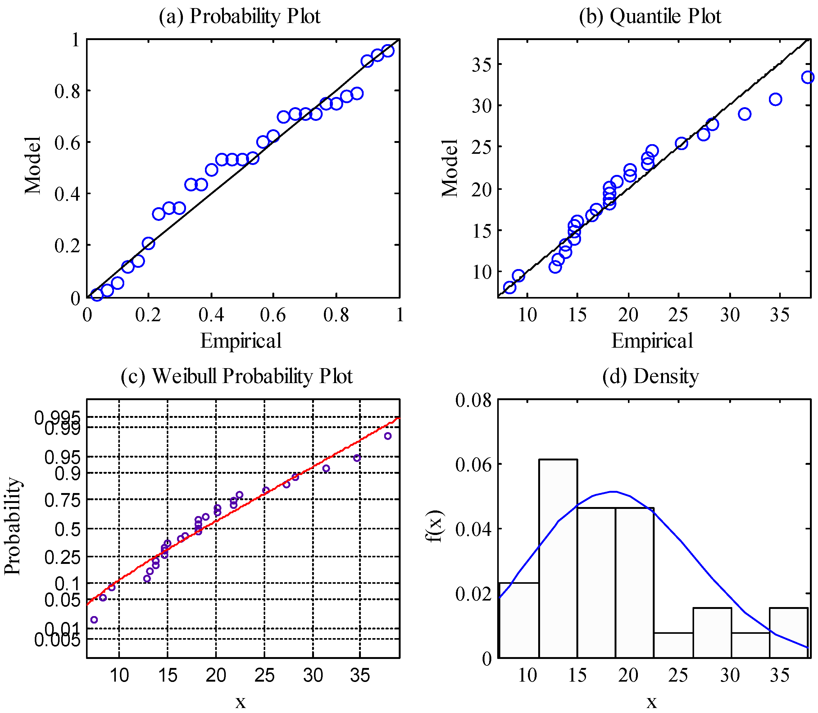
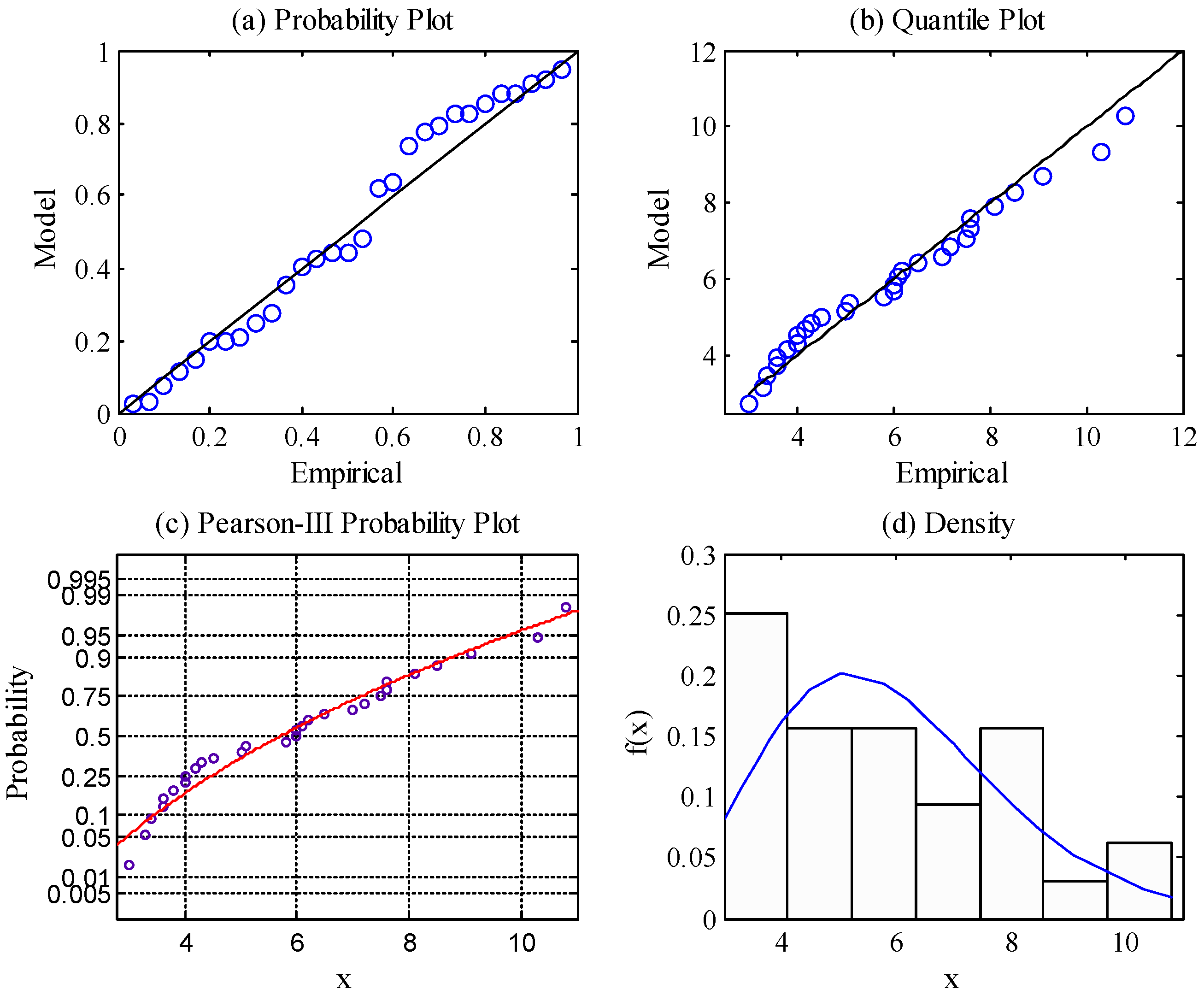
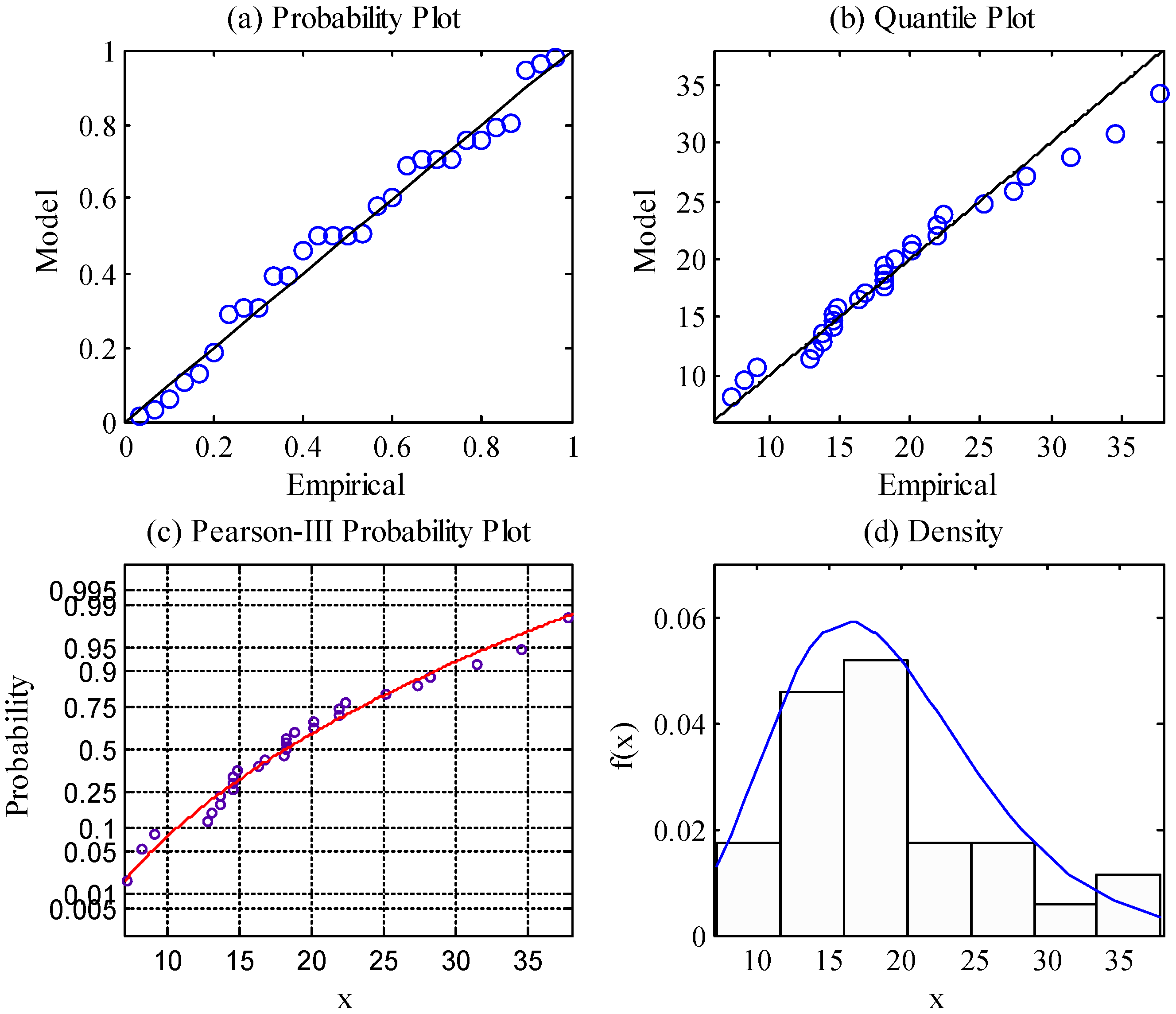
Figure 7, Figure 8, Figure 9, Figure 10, Figure 11 and Figure 12 show diagnostic tests including charts of probability, quantile, and return level (or a probability distribution plot) and a density histogram when using the Gumbel, Weibull, and Pearson-III distributions fitting of the annual extreme wave height and wind speed. The circles in the figures represent data points and solid lines that represent model curves.
The results of the corresponding diagnostic tests show that the annual extreme wave height and wind speed observation data comply with the Gumbel, Weibull, and Pearson-III distributions, and thus, the data can be used as analysis samples of the corresponding extreme value distribution.
Table 2 and Table 3 present interval estimates of the 95% confidence levels when using the Gumbel, Weibull, and Pearson-III distributions fitting of the annual extreme wave height and wind speed.
As shown in Table 2 and Table 3, it can be seen that, when the maximum entropy distribution is used to describe the annual extreme wave height, the P-Value is the maximum. Additionally, when describing the wind speed with Gumbel distribution, the P-Value is the maximum. Therefore, it is most appropriate to use the maximum entropy distribution to describe the annual extreme wave height, and use Gumbel distribution to describe the wind speed.
According to this, the two-dimensional joint distribution functions constructed by Gumbel-Hougaard Copula function and Clayton Copula function can be obtained. The joint distribution functions are as follows:
When the joint distribution of annual extreme wave height and wind speed is described with the mixed Gumbel distribution and Gumbel-Logistic distribution as well as Equations (14) and (15), three-dimensional contour plot of the corresponding distribution function is shown in Figure 13. The corresponding two-dimensional contour plot is shown in Figure 14.
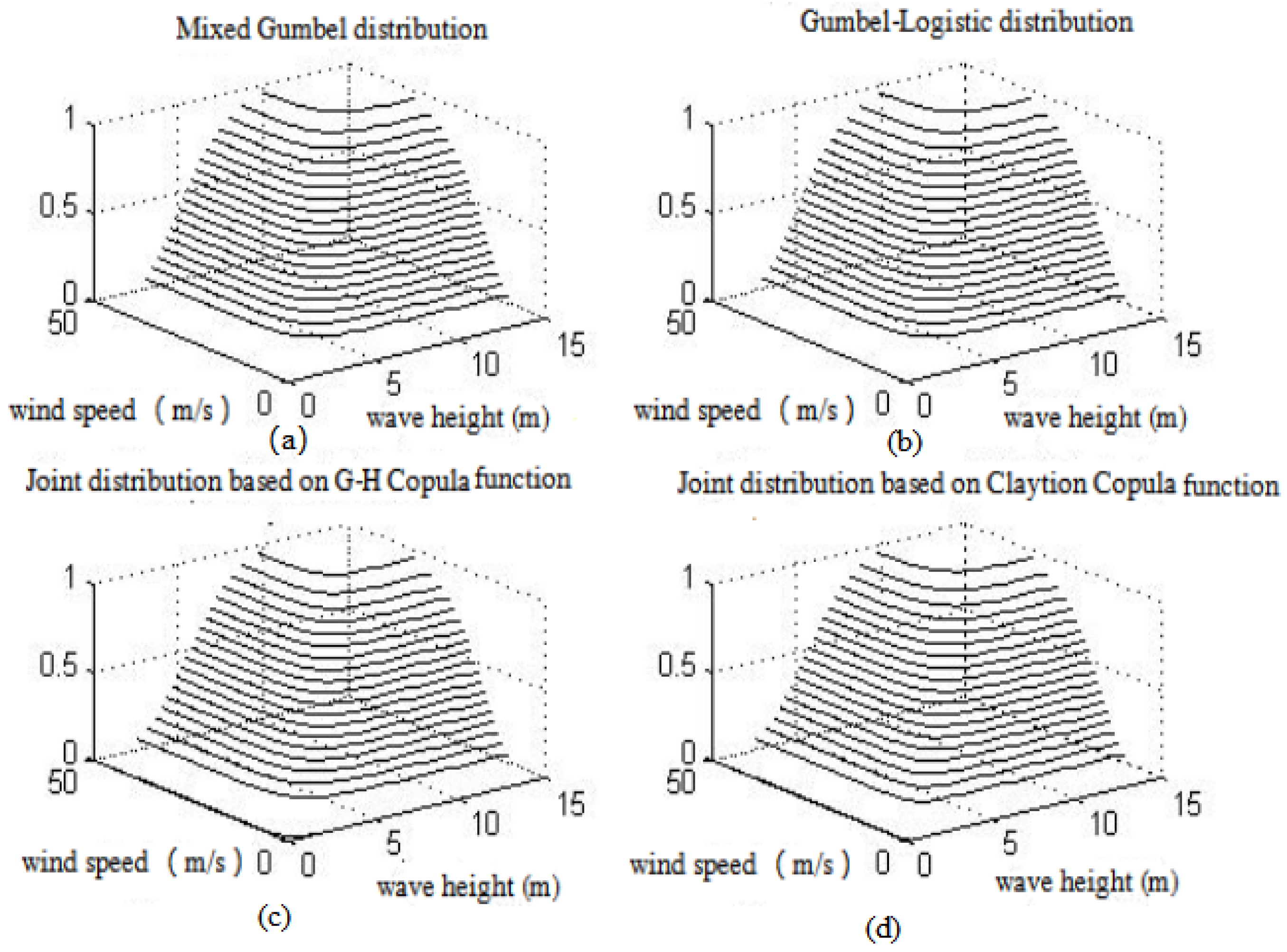
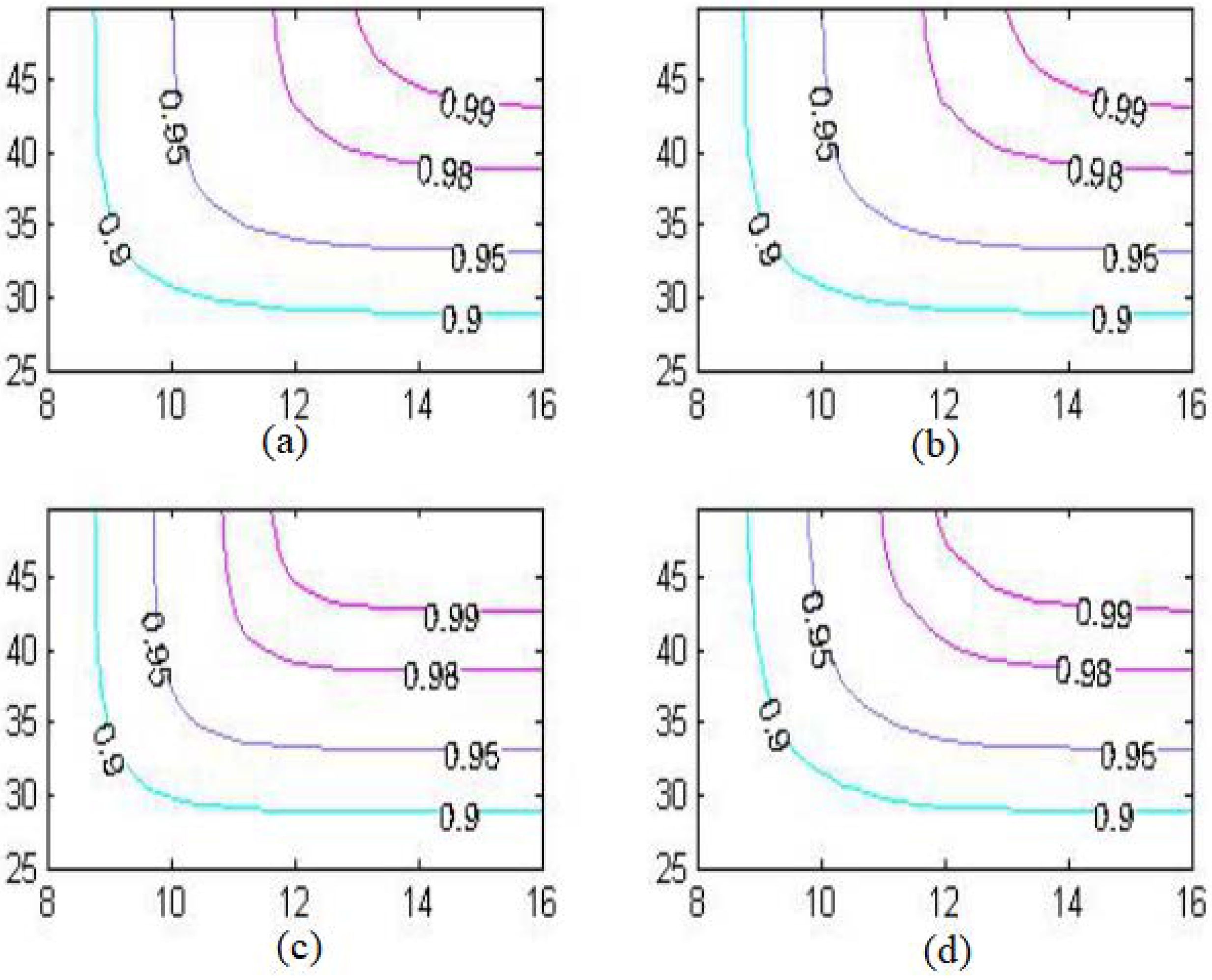
As shown in Figure 13, it can be seen that the shape of the four distribution function plots has little difference. Considering that mixed Gumbel and Gumbel-logistic distributions have been applied many times to different hydrological probabilistic analysis, the two established joint distributions based on Copula functions are similar to them, which are of a certain practical value in engineering application as well. Figure 14 shows a certain difference, especially when the joint probability exceeds 0.95, there are some differences between their contour. The mixed Gumbel distribution and Gumbel-Logistic distributions are steeper than the two distributions based on the Gumbel-Hougaard Copula function and Clayton Copula function. That means that when comparing with the established joint distributions, the traditional joint distributions can not fit the tail data very well. Namely, the multiyear return values calculated by the traditional joint distributions will be slightly larger. In the actual projects, the design parameters in the traditional joint distributions will bring a lot of unnecessary economic cost, and that the newly established joint distributions will be more reasonable and directly improve the economic benefits of projects.
4. The Joint Return Period Analysis
When analyzing two wave elements, we usually pay attention to the following two events, {X > x} and {Y > y}. Therefore, the joint return period can be defined as:
When the joint distribution of annual extreme wave height and wind speed is described with the mixed Gumbel distribution and Gumbel-Logistic distribution, as well as Equations (14) and (15), the multiyear design value and its joint return period of a single factor can be calculated, respectively. Table 4, Table 5, Table 6 and Table 7 shows them, respectively.
Table 4, Table 5, Table 6 and Table 7 present the joint return period calculated by the above four joint distributions, respectively, with the design wave height values and design wind speed values in 100, 200, 500, and 1000 year return periods. Obviously, the joint return periods of annual extreme wave height and wind speed are larger than that of single variable. The joint return periods calculated by the joint distributions that was constructed by the Gumbel-Hougaard Copula function and Clayton Copula function are lower than that calculated by the mixed Gumbel distribution and the Gumbel-Logistic distribution. In terms of the conservation of ocean engineering construction, the joint distribution of the Gumbel-Hougaard Copula function and Clayton Copula function are more reasonable.
After constructing the joint distribution of annual extreme wave height and wind speed with the Copula function, some design criteria for ocean engineering can be determined through joint return period analysis and conditional probability analysis. This provides a theoretical basis for the construction of ocean engineering, which can well control the construction cost of ocean engineering and ensure its safety in theory.
5. Conclusions
In this paper, the two-dimensional joint distributions of annual extreme wave height and corresponding wind speed in Weizhou Island from 1961 to 1989 are constructed by using the Gumbel-Hougaard (GH) Copula function and Clayton Copula function. The established models are compared with the commonly used two-dimensional joint distribution, mixed Gumbel distribution and Gumbel-Logistic distribution. Then the joint return period analysis and conditional probability analysis are analyzed by the two-dimensional joint distributions constructed by the Gumbel-Hougaard (GH) Copula function and Clayton Copula function. The conclusions are summarized as follows:
- (1)
- The multivariate joint distribution constructed by Copula function is more flexible than the common multivariate joint distribution in terms of marginal distribution. The common multivariate joint distributions usually require the marginal distribution to be specific.
- (2)
- The multivariate joint distribution constructed by the Copula function can better describe the non-normality of single variable, and combine multiple non-normal wave elements.
- (3)
- The marginal distribution of multivariate joint distribution constructed by Copula function is easy to be determined. Thus, it is easier to be realized in the joint return period analysis, especially in conditional probability analysis.
Author Contributions
Conceptualization, G.L.; Methodology, B.C. and L.W.; Software, S.J. and Z.G.; Validation, H.F. and K.L.; Formal Analysis, G.L.; Data Curation, L.W. and S.J.; Writing—Original Draft Preparation, G.L. and B.C.; Writing—Review and Editing, K.Y. and Z.G.; Visualization, S.J., L.W. and Z.G.; Supervision, B.C.; Project Administration, L.W. and K.Y.; and Funding Acquisition, H.F.
Funding
This research was funded by the NSFC--Shandong Joint Fund “Study on the Disaster-Causing Mechanism and Disaster Prevention Countermeasures of Multi-Source Storm Surges” (No. U1706226), and the Program of Promotion Plan for Postgraduates’ Educational Quality “Paying More Attention to the Study on the Cultivation Mode of Mathematical Modeling for Engineering Postgraduates” (No. HDJG18007)
Conflicts of Interest
The authors declare no conflict of interest.
References
- Wang, L.P.; Chen, B.Y.; Chen, C.; Chen, Z.S.; Liu, G.L. Application of linear mean-square estimation in ocean engineering. China Ocean Eng. 2016, 30, 149–160. [Google Scholar] [CrossRef]
- Wang, L.P.; Xu, X.; Liu, G.L.; Chen, B.Y.; Chen, Z.S. A new method to estimate wave height of specified return period. Chin. J. Oceanol. Limnol. 2017, 35, 1002–1009. [Google Scholar] [CrossRef]
- Chen, B.Y.; Liu, G.L.; Wang, L.P.; Zhang, K.Y; Zhang, S.F. Determination of Water Level Design for an Estuarine City. J. Oceanol. Limnol. 2018. [CrossRef]
- Chen, B.Y.; Zhang, K.Y.; Wang, L.P.; Jiang, S.; Liu, G.L. Generalized Extreme Value-Pareto Distribution Function and Its Applications in Ocean Engineering. China Ocean Eng. 2019, 2. in press. [Google Scholar]
- Wang, L.P.; Chen, B.Y; Zhang, J.F.; Chen, Z.S. A new model for calculating the design wave height in typhoon-affected sea areas. Nat. Hazards 2013, 67, 129–143. [Google Scholar] [CrossRef]
- Chen, B.Y.; Liu, G.L.; Wang, L.P. Predicting Joint Return Period Under Ocean Extremes Based on a Maximum Entropy Compound Distribution Model. Int. J. Energy Environ. Sci. 2017, 2, 117–126. [Google Scholar]
- Chen, B.Y.; Liu, G.L.; Zhang, J.F. A Calculation Method of Design Wave Height under the Three Factors of Typhoon. China Patent CN201610972118, 29 August 2017. [Google Scholar]
- Wang, L.P.; Liu, G.L.; Chen, B.Y.; Wang, L. Typhoon Influence Considered Method for Calculating Combined Return Period of Ocean Extreme Value. China Patent CN201010595807.6, 20 March 2013. [Google Scholar]
- Liu, G.L.; Zheng, Z.J.; Wang, L.P.; Chen, B.Y.; Dong, X.J.; Xu, P.Y.; Wang, J.; Wang, C. Power-Type Wave Absorbing Device and Using Method Thereof. China Patent 2015. [Google Scholar]
- Chen, B.Y.; Yang, Z.Y.; Huang, S.Y.; Du, X.Z.; Cui, Z.W.; Bhimani, J.; Xie, X.; Mi, N.F. Cyber-physical system enabled nearby traffic flow modelling for autonomous vehicles. In Proceedings of the IEEE 36th IEEE International Performance Computing and Communications Conference (IPCCC), San Diego, CA, USA, 10–12 December 2017; pp. 1–6. [Google Scholar]
- Escalante, H.J.; Ponce-López, V.; Wan, J.; Riegler, M.A.; Chen, B.Y.; Clapés, A.; Escalera, S.; Guyon, I.; Baró, X.; Halvorsen, P.; et al. ChaLearn joint contest on multimedia challenges beyond visual analysis: An overview. In Proceedings of the 23rd International Conference on Pattern Recognition (ICPR), Cancun, Mexico, 4–8 December 2016; pp. 67–73. [Google Scholar]
- Barrs, A.; Chen, B.Y. How Emerging Technologies Could Transform Infrastructure. Available online: http://www.governing.com/commentary/col-hyperlane-emerging-technologies-transform-infrastructure.html (accessed on 10 March 2018).
- Chen, B.Y.; Escalera, S.; Guyon, I.; Ponce-López, V.; Shah, N.; Simón, M.O. Overcoming calibration problems in pattern labeling with pairwise ratings: Application to personality traits. In Computer Vision—ECCV 2016 Workshops; Hua, G., Jégou, H., Eds.; Springer: Amsterdam, The Netherlands, 2016; pp. 419–432. [Google Scholar]
- Ponce-López, V.; Chen, B.Y.; Oliu, M.; Corneanu, C.; Clapés, A.; Guyon, I.; Baró, X.; Escalante, H.J.; Escalera, S. ChaLearn LAP 2016: First round challenge on first impressions-dataset and results. In Computer Vision-ECCV 2016 Workshops; Hua, G., Jégou, H., Eds.; Springer: Amsterdam, The Netherlands, 2016; pp. 400–418. [Google Scholar]
- Zhang, S.F.; Shen, W.; Li, D.S.; Zhang, X.W.; Chen, B.Y. Nondestructive ultrasonic testing in rod structure with a novel numerical Laplace based wavelet finite element method. Latin Am. J. Solids Struct. 2018, 15, e48. [Google Scholar] [CrossRef]
- Chen, B.Y.; Wang, B.Y. Location Selection of Logistics Center in e-Commerce Network Environments. Am. J. Neural Netw. Appl. 2017, 3, 40–48. [Google Scholar] [CrossRef]
- Wang, L.P.; Liu, G.L.; Chen, B.Y.; Wang, L. Typhoon Based on the Principle of Maximum Entropy Waters Affect the Design Wave Height Calculation Method. China Patent CN201010595815, 20 December 2010. [Google Scholar]
- Du, Q.; Lu, X.; Li, Y.; Wu, M.; Bai, L.; Yu, M. Carbon Emissions in China’s Construction Industry: Calculations, Factors and Regions. Int. J. Environ. Res. Public Health 2018, 15, 1220. [Google Scholar] [CrossRef]
- Yang, A.M.; Li, S.S.; Lin, H.L.; Jin, D.H. Edge Extraction of Mineralogical Phase Based on Fractal Theory. Chaos Solitions Fractals 2018, 117, 215–221. [Google Scholar]
- Liu, X.J.; He, Y.Q.; Fu, H.L.; Chen, B.Y.; Wang, M.; Wang, Z. How Environmental Protection Motivation Influences on Residents’ Recycled Water Reuse Behaviors: A Case Study in Xi’an City. Water 2018, 10, 1282. [Google Scholar] [CrossRef]
- Liu, G.L.; Chen, B.Y.; Wang, L.P.; Zhang, S.F.; Zhang, K.Y.; Lei, X. Wave height statistical characteristic analysis. Oceanol. Limnol. 2018. [Google Scholar] [CrossRef]
- Yue, S. The Gumbel Mixed Model Applied to Storm Frequency Analysis. Water Resour. Manag. 2000, 14, 377–389. [Google Scholar] [CrossRef]
- Zhou, D.C.; Duan, Z.D. The Gumbel-logistic model for joint probability distribution of extreme-value wind speeds and effective wave heights. Ocean Eng. 2003, 21, 45–51. [Google Scholar]
- Dong, S.; Cong, J.S.; Yu, H.J. Design Parameter Estimation of Joint Extreme Significant Wave Height and Wind Speed at Weizhoudao Observation Station. Period Ocean Univ. China 2006, 36, 489–492. [Google Scholar]
- Liu, X.; Wang, M.; Fu, H. Visualized analysis of knowledge development in green building based on bibliographic data mining. J. Supercomput. 2018. [Google Scholar] [CrossRef]
- Jiang, S.; Lian, M.J.; Lu, C.W.; Ruan, S.L.; Wang, Z.; Chen, B.Y. SVM-DS fusion based soft fault detection and diagnosis in solar water heaters. Energy Explor. Exploit. 2018. [Google Scholar] [CrossRef]
- Jiang, S.; Lian, M.J.; Lu, C.W; Gu, Q.H; Ruan, S.L.; Xie, X.C. Ensemble Prediction Algorithm of Anomaly Monitoring Based on Big Data Analysis Platform of Open-Pit Mine Slope. Complexity 2018, 2018, 1048756. [Google Scholar] [CrossRef]
- Chen, B.; Liu, G.; Wang, L.; Zhang, K.; Zhang, S. Determination of Water Level Design for an Estuarine City. J. Oceanol. Limnol. 2019. [Google Scholar] [CrossRef]
- Yang, A.M.; Yang, X.L.; Wu, W.R.; Liu, H.X.; Zhuansun, Y.X. Research on Feature Extraction of Tumor Image Based on Convolutional Neural Network. IEEE Access 2019. [Google Scholar] [CrossRef]
- Skla, A. Fonctions de repartition a n dimensions et leurs marges. Publ. Inst. Statist. Univ. Paris 1959, 8, 229–231. [Google Scholar]
- Deng, W.; Yao, R.; Zhao, H.M.; Yang, X.H.; Li, G.Y. A novel intelligent diagnosis method using optimal LS-SVM with improved PSO algorithm. Soft Comput. 2017. [Google Scholar] [CrossRef]
- Deng, W.; Zhao, H.M.; Yang, X.H.; Xiong, J.X.; Sun, M.; Li, B. Study on an improved adaptive PSO algorithm for solving multi-objective gate assignment. Appl. Soft Comput. 2017, 59, 288–302. [Google Scholar] [CrossRef]
- Deng, W.; Zhao, H.M.; Zou, L.; Li, G.Y.; Yang, X.H.; Wu, D.Q. A novel collaborative optimization algorithm in solving complex optimization problems. Soft Comput. 2017, 21, 4387–4398. [Google Scholar] [CrossRef]
- Liu, G.; Chen, B.; Jiang, S.; Fu, H.; Wang, L.; Jiang, W. Double Entropy Joint Distribution Function and Its Application in Calculation of Design Wave Height. Entropy 2019, 21, 64. [Google Scholar] [CrossRef]
- Kang, L.; Du, H.L.; Zhang, H.; Ma, W.L. Systematic research on the application of steel slag resources under the background of big data. Complexity 2018, 2018, 6703908. [Google Scholar] [CrossRef]
- Song, J.; Feng, Q.; Wang, X.; Fu, H.; Jiang, W.; Chen, B. Spatial Association and Effect Evaluation of CO2 Emission in the Chengdu-Chongqing Urban Agglomeration: Quantitative Evidence from Social Network Analysis. Sustainability 2019, 11, 1. [Google Scholar] [CrossRef]
- Deng, W.; Zhang, S.J.; Zhao, H.M.; Yang, X.H. A novel fault diagnosis method based on integrating empirical wavelet transform and fuzzy entropy for motor bearing. IEEE Access 2018, 6, 35042–35056. [Google Scholar] [CrossRef]
- Zhao, H.M.; Yao, R.; Yu, L.X.; Xu, L.; Li, G.Y.; Deng, W. Study on a novel fault damage degree identification method using high-order differential mathematical morphology gradient spectrum entropy. Entropy 2018, 20, 682. [Google Scholar] [CrossRef]
- Zhao, H.M.; Sun, M.; Deng, W.; Yang, X.H. A new feature extraction method based on EEMD and multi-scale fuzzy entropy for motor bearing. Entropy 2017, 19, 14. [Google Scholar] [CrossRef]
Figure 1.
Scatter diagrams of the two Copula functions. (a)the Gumbel-Hougaard (GH) Copula function; (b) the Clayton Copula function.
Figure 1.
Scatter diagrams of the two Copula functions. (a)the Gumbel-Hougaard (GH) Copula function; (b) the Clayton Copula function.

Figure 2.
Gumbel-Hougaard (GH) Copula function: (a) θ = 2, and (b) θ = 6.

Figure 3.
Gumbel-Hougaard (GH) Copula density function: (a) θ = 2, and (b) θ = 6.

Figure 4.
Clayton Copula function: (a) θ = 2, and (b) θ = 6.

Figure 5.
Clayton Copula density function: (a) θ = 2, and (b) θ = 6.

Figure 6.
The scatter plot of the annual extreme wave height and corresponding wind.

Figure 7.
Gumbel distribution of the annual extreme wave height: (a) Probability, (b) quantile, (c) return level, and (d) density.
Figure 7.
Gumbel distribution of the annual extreme wave height: (a) Probability, (b) quantile, (c) return level, and (d) density.

Figure 8.
Gumbel distribution of the wind speed: (a) Probability, (b) quantile, (c) return level, and (d) density.
Figure 8.
Gumbel distribution of the wind speed: (a) Probability, (b) quantile, (c) return level, and (d) density.

Figure 9.
Weibull distribution of the annual extreme wave height: (a) Probability, (b) quantile, (c) Weibull probability distribution, and (d) density.
Figure 9.
Weibull distribution of the annual extreme wave height: (a) Probability, (b) quantile, (c) Weibull probability distribution, and (d) density.

Figure 10.
Weibull distribution of the wind speed: (a) Probability, (b) quantile, (c) Weibull probability distribution, and (d) density.
Figure 10.
Weibull distribution of the wind speed: (a) Probability, (b) quantile, (c) Weibull probability distribution, and (d) density.

Figure 11.
Pearson-III distribution of the annual extreme wave height: (a) Probability, (b) quantile, (c) Pearson-III probability distribution, and (d) density.
Figure 11.
Pearson-III distribution of the annual extreme wave height: (a) Probability, (b) quantile, (c) Pearson-III probability distribution, and (d) density.

Figure 12.
Pearson-III distribution of the wind speed: (a) Probability, (b) quantile, (c) Pearson-III probability distribution, and (d) density.
Figure 12.
Pearson-III distribution of the wind speed: (a) Probability, (b) quantile, (c) Pearson-III probability distribution, and (d) density.

Figure 13.
The above four joint distribution function plots: (a) mixed Gumbel distribution, (b) Gumbel-Logistic distribution, (c) joint distribution based on G-H Copula function, and (d) joint distribution based on Clayton Copula function.
Figure 13.
The above four joint distribution function plots: (a) mixed Gumbel distribution, (b) Gumbel-Logistic distribution, (c) joint distribution based on G-H Copula function, and (d) joint distribution based on Clayton Copula function.

Figure 14.
The above four joint distribution function contour plots: (a) mixed Gumbel distribution, (b) Gumbel-Logistic distribution, (c) joint distribution based on G-H Copula function, and (d) joint distribution based on Clayton Copula function.
Figure 14.
The above four joint distribution function contour plots: (a) mixed Gumbel distribution, (b) Gumbel-Logistic distribution, (c) joint distribution based on G-H Copula function, and (d) joint distribution based on Clayton Copula function.


Table 1.
The linear correlation coefficient and rank correlation coefficient.
| Correlation Coefficients | Linear Correlation Coefficient ρ | Rank Correlation Coefficient τ |
|---|---|---|
| The annual extreme wave height and corresponding wind speed | 0.4992 | 0.383 |
Table 2.
K-S test of the annual extreme wave height distribution function.
| Distribution Functions | Gumbel Distribution | Weibull Distribution | Person-Ⅲ Distribution | Maximum Entropy Distribution |
|---|---|---|---|---|
| P-Value | 0.8158 | 0.7854 | 0.7728 | 0.8200 |
| Ksstat | 0.1127 | 0.1163 | 0.1178 | 0.1122 |
Table 3.
K-S test of the wind speed distribution function.
| Distribution Functions | Gumbel Distribution | Weibull Distribution | Person-Ⅲ Distribution | Maximum Entropy Distribution |
|---|---|---|---|---|
| P-Value | 0.9496 | 0.7313 | 0.9464 | 0.9031 |
| Ksstat | 0.0916 | 0.1225 | 0.0923 | 0.1005 |
Table 4.
Design wave height (m) and design wind speed (m/s) in different return periods based on the mixed Gumbel distribution.
Table 4.
Design wave height (m) and design wind speed (m/s) in different return periods based on the mixed Gumbel distribution.
| Return Period | Marginal Distribution Design Value | ||
|---|---|---|---|
| T (a Single Variable) | T0 | T (a Single Variable) | T0 |
| 100 | 258 | 100 | 258 |
| 200 | 518 | 200 | 518 |
| 500 | 1302 | 500 | 1302 |
| 1000 | 2605 | 1000 | 2605 |
Table 5.
Design wave height (m) and design wind speed (m/s) in different return periods based on the Gumbel-Logistic distribution.
Table 5.
Design wave height (m) and design wind speed (m/s) in different return periods based on the Gumbel-Logistic distribution.
| Return Period | Marginal Distribution Design Value | ||
|---|---|---|---|
| T (a Single Variable) | T0 | T (a Single Variable) | T0 |
| 100 | 269 | 100 | 269 |
| 200 | 540 | 200 | 540 |
| 500 | 1358 | 500 | 1358 |
| 1000 | 2718 | 1000 | 2718 |
Table 6.
Design wave height (m) and design wind speed (m/s) in different return periods based on the G-H Copula distribution.
Table 6.
Design wave height (m) and design wind speed (m/s) in different return periods based on the G-H Copula distribution.
| Return Period | Marginal Distribution Design Value | ||
|---|---|---|---|
| T (a Single Variable) | T0 | T (a Single Variable) | T0 |
| 100 | 198 | 100 | 198 |
| 200 | 381 | 200 | 381 |
| 500 | 966 | 500 | 966 |
| 1000 | 2087 | 1000 | 2087 |
Table 7.
Design wave height (m) and design wind speed (m/s) in different return periods based on the Clayton Copula distribution.
Table 7.
Design wave height (m) and design wind speed (m/s) in different return periods based on the Clayton Copula distribution.
| Return Period | Marginal Distribution Design Value | ||
|---|---|---|---|
| T (a Single Variable) | T0 | T (a Single Variable) | T0 |
| 100 | 201 | 100 | 201 |
| 200 | 390 | 200 | 390 |
| 500 | 981 | 500 | 981 |
| 1000 | 2072 | 1000 | 2072 |
© 2019 by the authors. Licensee MDPI, Basel, Switzerland. This article is an open access article distributed under the terms and conditions of the Creative Commons Attribution (CC BY) license (http://creativecommons.org/licenses/by/4.0/).
Share and Cite
MDPI and ACS Style
Liu, G.; Chen, B.; Gao, Z.; Fu, H.; Jiang, S.; Wang, L.; Yi, K. Calculation of Joint Return Period for Connected Edge Data. Water 2019, 11, 300. https://doi.org/10.3390/w11020300
AMA Style
Liu G, Chen B, Gao Z, Fu H, Jiang S, Wang L, Yi K. Calculation of Joint Return Period for Connected Edge Data. Water. 2019; 11(2):300. https://doi.org/10.3390/w11020300
Chicago/Turabian StyleLiu, Guilin, Baiyu Chen, Zhikang Gao, Hanliang Fu, Song Jiang, Liping Wang, and Kou Yi. 2019. "Calculation of Joint Return Period for Connected Edge Data" Water 11, no. 2: 300. https://doi.org/10.3390/w11020300
Note that from the first issue of 2016, this journal uses article numbers instead of page numbers. See further details here.