Analysis of Drought Progression Physiognomies in South Africa
by
 , and
, and
Joel Ondego Botai
1,2,3,*, 
Christina M. Botai
1, 
Jaco P. de Wit
1,
Masinde Muthoni
4 and
Abiodun M. Adeola
1,5 1
South African Weather Service, Private Bag X097, Pretoria 0001, South Africa
2
Department of Geography, Geoinformatics and Meteorology, University of Pretoria, Private Bag X020, Hatfield 0028, South Africa
3
School of Agricultural, Earth and Environmental Sciences, University of KwaZulu-Natal, Westville Campus, Private Bag X54001, Durban 4000, South Africa
4
Department of Information Technology, Central University of Technology, Free State, Private Bag X200539, Bloemfontein 9300, South Africa
5
School for Health Systems and Public Health, University of Pretoria, Pretoria 0002, South Africa
*
Author to whom correspondence should be addressed.
Water 2019, 11(2), 299; https://doi.org/10.3390/w11020299
Submission received: 5 December 2018
/
Revised: 21 January 2019
/
Accepted: 26 January 2019
/
Published: 11 February 2019
(This article belongs to the Section Water Resources Management, Policy and Governance)
Abstract
:The spatial-temporal variability of drought characteristics and propagation mechanisms in the hydrological cycle is a pertinent topic to policymakers and to the diverse scientific community. This study reports on the analysis of drought characteristics and propagation patterns in the hydrological cycle over South Africa. In particular, the analysis considered daily precipitation and streamflow data spanning from 1985 to 2016, recorded from 74 weather stations, distributed across South Africa and covering the country’s 19 Water Management Areas (WMAs). The results show that all the WMAs experience drought features characterized by an inherent spatial-temporal dependence structure with transition periods categorized into short (1–3 months), intermediate (4–6 months), long (7–12 months) and extended (>12 months) time-scales. Coupled with climate and catchment characteristics, the drought propagation characteristics delineate the WMAs into homogenous zones subtly akin to the broader climatic zones of South Africa, i.e., Savanna, Grassland, Karoo, Fynbos, Forest, and Desert climates. We posit that drought evolution results emanating from the current study provide a new perspective of drought characterization with practical use for the design of drought monitoring, as well as early warning systems for drought hazard preparedness and effective water resources planning and management. Overall, the analysis of drought evolution in South Africa is expected to stimulate advanced drought research topics, including the elusive drought termination typology.
1. Introduction
Drought is a slowly reoccurring, natural phenomenon with a complex development pattern. This natural hazard is often characterized as a deviation of weather and climate variations (and change) as manifested in parameters such as precipitation, soil moisture, groundwater, and streamflow from normal conditions. It exhibits spatial and temporal characteristics that vary significantly from one region to another. Unlike other hazards (e.g., floods), drought gradually develops over a broader area for a longer period of time and only becomes recognized after it is well developed [1]. Drought virtually occurs at all climate regions (both in dry and wet areas), although the most severe social consequences are often experienced in arid or semi-arid regions where the vulnerability is high as the availability of water is already low under normal conditions [2].
As it develops, drought begins as a meteorological drought progressing through a series of characteristics that include a lack of precipitation over a large area and for an extended period of time [3]. The deficit in precipitation coupled with higher evaporation rates propagates through every component of the hydrological cycle, giving rise to different types of droughts. For instance, a meteorological drought may propagate into soil moisture depletion up to a point where crops are impacted, thus leading to an agricultural phenomenon/drought or eventually to a hydrological phenomenon/drought that includes both groundwater and streamflow droughts [1,4,5]. Hydrological drought is attributed to low precipitation coupled with high evapotranspiration rates, which result in a recharge deficit, consequently lowering groundwater heads and streamflow as well as including a deficit in water reservoirs discharge (groundwater, lakes, rivers, dams, etc.) [1,4,6].
Drought propagation from one type to the other depends on the severity of the drought event, measured by regional characteristics such as the area covered by the drought and the total deficit over that area, as well as the characteristics of the catchments [7,8]. Climate processes, including multi-land-atmosphere feedback processes (linked to the frequency and occurrence of drought in a catchment), often complicate the propagation of the climate signal into the water system [7]. An early warning system for drought detection is an essential tool that can be used to monitor drought occurrence and mitigate its impact in a given area. However, the success of such a system requires that we understand and distinguish between different types of drought. In addition, understanding how drought propagates from one type to another is required for adequate seasonal and long-term drought forecasting.
Research studies devoted to understanding the occurrence and propagation of drought are still in the early stages of development. Nevertheless, interest in drought propagation in groundwater has increased over the years [9,10,11,12,13]. For instance, Reference [13] simulated the propagation of droughts through a groundwater system with the aim of assessing the effects of the drought propagation through a groundwater reservoir. Similar studies by Reference [14] simulated recharge, hydraulic heads, and groundwater discharge to analyze the propagation and spatial distribution of the drought in the groundwater system. Studies by Reference [8] analyzed rainfall and groundwater recharge time series data to investigate drought propagation within the Pang Catchment. As can be noted, most of these reported studies have focused on the propagation of groundwater drought rather than the streamflow drought. It can be therefore concluded that studies devoted to the occurrence and propagation of meteorological drought to hydrological drought, particularly the streamflow drought, are still limited.
To our knowledge, studies dwelling on the occurrence and propagation of drought in the hydrological cycle in South Africa are either non-existent or limited. Against this backdrop, the aim of this study is to analyze drought propagation in the hydrological cycle across South Africa. To achieve our aim, the following specific objectives are constructed: (a) To characterize the spatial-temporal drought patterns across all the South African Water Management Areas (WMAs), based on analysis of quartiles, standard deviation, and trends in drought metrics (i.e., drought duration and severity) derived from SPI-1, -3, -6, -12, -18, and -24 accumulation months; (b) to analyze the spatial variability of drought propagation periods across all the WMAs; and (c) to delineate South African catchments areas (WMAs) into small zones that exhibit self-similar drought propagation time scales using clustering.
2. Study Area, Materials, and Methods
2.1. Study Area
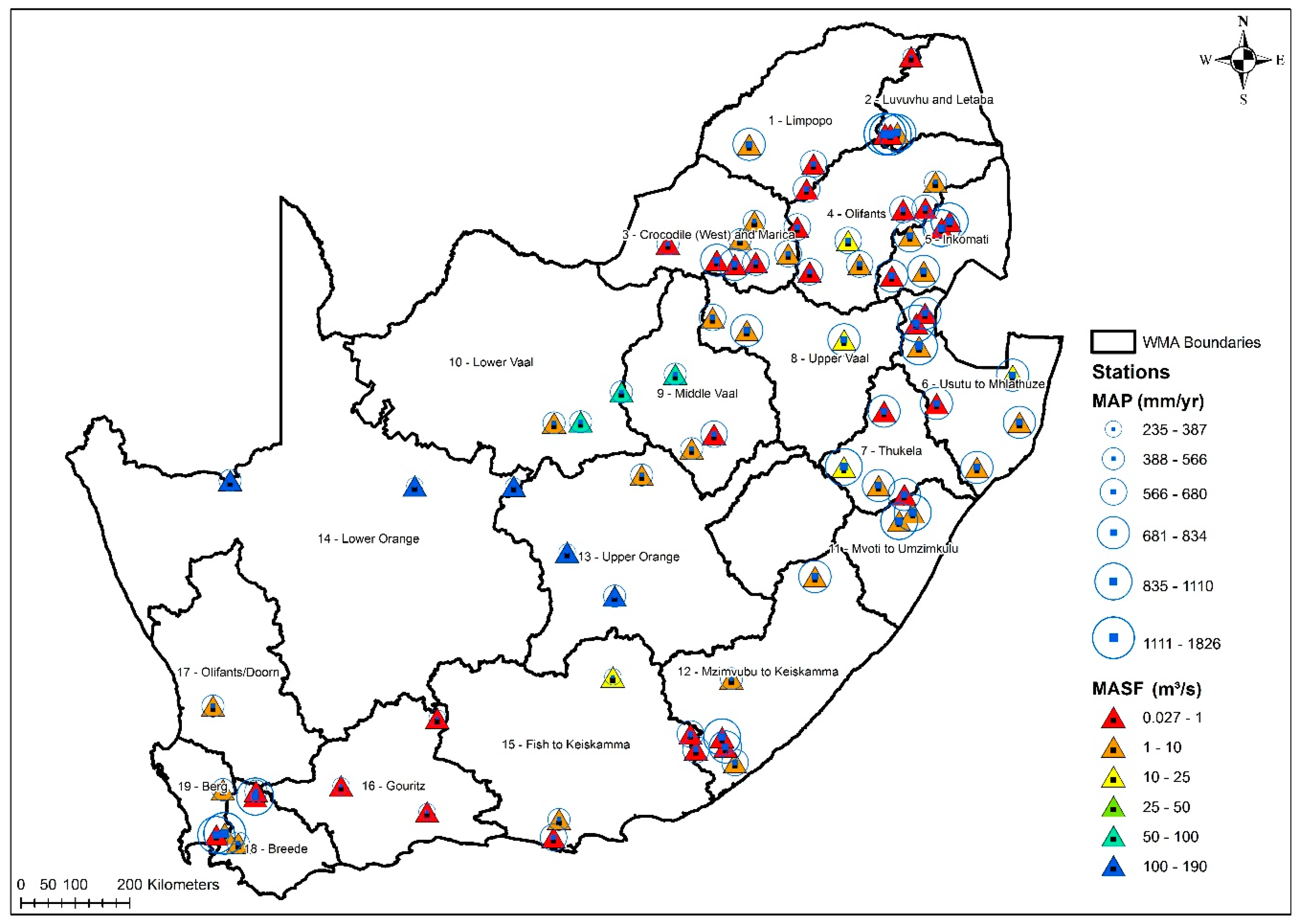
South Africa is located at the Southernmost part of the African continent. It has a surface area of 1,219,090 km2 and an extensive coastline of approximately 3200 km that is constituted of the Western, Southern and Eastern boundaries of the country. South Africa is considered as a semi-arid to arid country and it is characterized by spatial and temporal rainfall variability ranging from as high as 1000 mm/year to less than 250 mm/year. The average annual rainfall is recorded at about 450 mm/year, which is far less compared to the world’s average annual rainfall (e.g., 860 mm/year). The rainfall is received at different timescales across the country, although the vast majority of the country receives rainfall during the summer season (i.e., December, January, and February). The Southwestern (around Cape Town) region of South Africa is highly characterized by winter rainfall, whereas the Northwestern regions receive rainfall all year. In particular, the whole western coast receives winter rainfall characterized by frontal systems which often occur when the cold fronts move north. In South Africa, water resources are mainly the rivers, dams, lakes, wetlands, groundwater, and subsurface aquifers. These water resources are currently partitioned into 19 WMAs, covering the nine South African provinces. The distribution and salient features of the WMAs across the different provinces are depicted in Figure 1 and Table 1 (excerpts only), respectively.
2.2. Materials
Historical time series (1985–2016) of daily precipitation and streamflow data from 74 weather stations distributed across the 19 WMAs of South Africa were selected for the drought propagation analysis. All the 74 weather stations are operated by the South African government under the Department of Water and Sanitation (DWS). These weather stations were selected based on the availability of continuous rainfall records for the considered 31 years. In addition, the weather stations are relatively evenly distributed throughout the WMAs study region and exhibited less than 5% missing data. Similarly, for the streamflow data, stations were selected based on the availability of continuous data, the proximity of the stations to the rainfall weather stations, and their distribution across the WMAs study region. The summary of the selected rainfall weather and streamflow gauge stations is provided in Table 2 as well as in Figure 2 (which also depict the Mean Annual Stream Flow and Mean Annual Precipitation, hereafter MASF and MAP respectively).
2.3. Methods
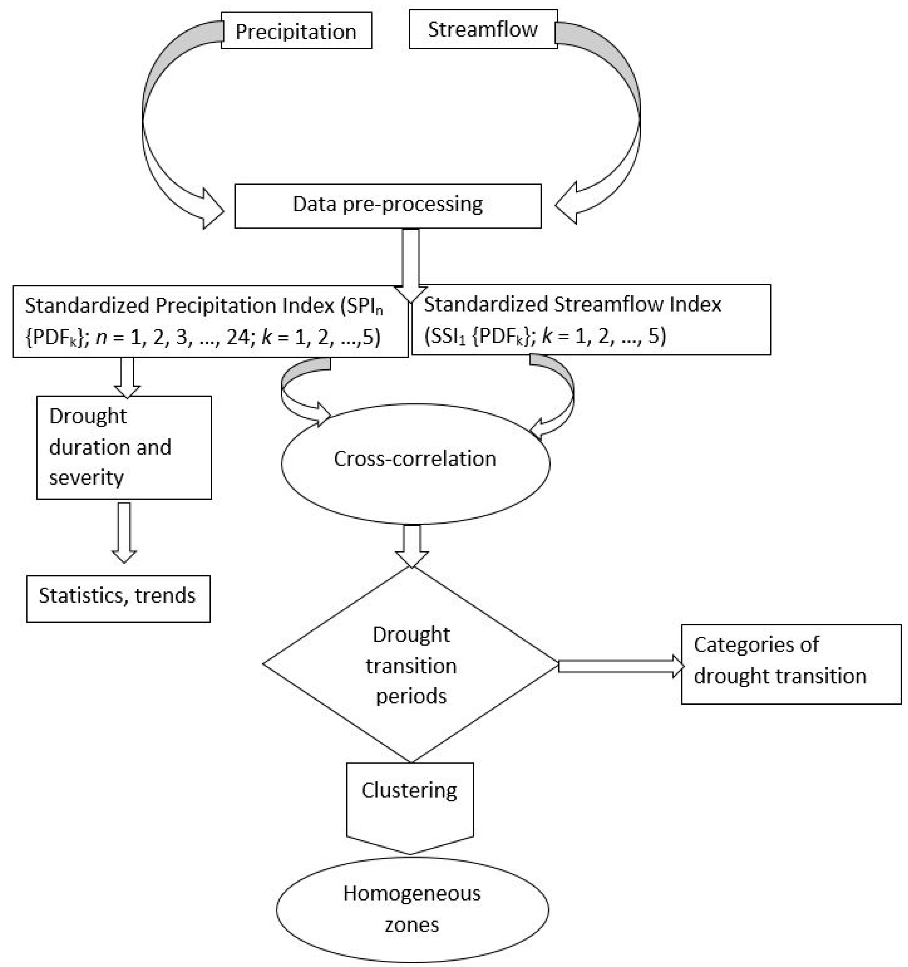
The methodology utilized in the present study is illustrated in Figure 3. The details of some of the processing and analysis methods are given in the subsequent sub-sections.
2.3.1. Calculation of Drought Indicators
Standardized Precipitation Index (SPI) and Standardized Streamflow Index (SSI)
In this research, a methodology reported in References [15,16,17,18,19] was used to compute the SPI-n (where n = 1, 2, 3, …, 24 months) time series. In particular, the SPI-n and SSI-1 time series were calculated by fitting five different probability distributions (see Table 3) to accumulated monthly precipitation and streamflow time series, for each rainfall and discharge gauging station. The corresponding probability distribution parameters for each station for the SPI-n and SSI-1 accumulation months were estimated and then transformed into a normal distribution (i.e., µ = 0, σ = 1), resulting in SPI-n and SSI-1 values. Negative values indicate wetter conditions whereas positive values indicate drier conditions. Overall, the SPI/SSI computation entails the following algorithm:
- (a)
- Fitting a probability function of the candidate distribution (given in Table 3) to a frequency distribution of accumulated monthly precipitation and streamflow.
- (b)
- Use the maximum likelihood solutions to estimate the corresponding two- and three-parameter values of the distribution functions.
- (c)
- For each candidate distribution, compute the cumulative probability using the parameters estimated in (b).
- (d)
- Compute the SPI by transforming the cumulative probability computed in (c) to a standard normal random variable, Z. As such, Z (and therefore SPI) has a mean of zero and a variance of one.
Drought Transition Periods
The derived time series (i.e., SPI-n and SSI-1) were analyzed to determine drought propagation time scales across different WMAs. The drought propagation analysis was carried out by cross-correlating SSI-1 time series with SPI-n time series by considering accumulation periods of 1–24 months using the Pearson correlation coefficient. The SPI accumulation period with the strongest correlation with the SSI-1 was used as an indicator for the drought transition period. For more information on the Pearson correlation coefficient analysis method, the reader is referred to References [18,19], and the references therein.
2.3.2. Cluster Analysis
Assessment of Clustering Tendency
As reported in Reference [20], before clustering catchment datasets, it is vital that an assessment is done to determine if the dataset exhibits a predisposition to cluster into natural groups without identifying the groups themselves. In the assessment, the Hopkins statistic reported in Reference [20] was used to measure the probability that the dataset exhibits uniform distribution. The algorithm used can be summarized as follows:
- Sample uniform k data points randomly from X: {x1, x2,…,xk}. For each data point xi (and the nearest data point xj), the distance dxi between xi and xj is computed using Equation (1).
- Using the first order statistical moments of X (i.e., the mean and variance), we derive a randomly simulated dataset, Y.
- Repeat step 2 using Equation (1) and derive dyi.
- Calculate the Hopkins statistic (H) using Equation (2)
We posit that if X is uniformly distributed, then
Given the result in step 5, the null and alternative hypothesis can be postulated as follows:
- Null hypothesis: X is uniformly distributed and therefore no clusters are present.
- Alternative hypothesis: X is not uniformly distributed hence clusters are present.
A value of H = 0.5 is then used as a threshold to reject the alternative hypothesis. In this regard, if H < 0.5, it is unlikely for X to exhibit statistically significant clusters. Stated differently, if H ~ 1.0, the null hypothesis is rejected, and thus X is statistically clusterable.
Determining the Optimal Number of Clusters
While it is generally known that determining the appropriate number of clusters in datasets is a subjective exercise, in the present work, the optimal number of clusters in the datasets was determined using the methodology described in Reference [21] and developed as an NbClust R package. As reported in Reference [22], the best clustering scheme is selected based on various combinations of the number of clusters, distance measures, and the clustering methods (whether direct or test methods).
Assessment of Clustering Method
Different methods of clustering have been proposed in the literature and the choice of the most suitable method is often not a trivial task. In this paper, the R package clValid [23] was used to compare the two commonly used clustering methods, namely K-means and hierarchical clustering. In particular, the K-means clustering partitions the data into k clusters iteratively. In general, the K-means procedure is as follows:
- (a)
- For a set of data points with dimension d; , initialize the k center, with a value,
- (b)
- Using, e.g., the Manhattan distance measure, i.e., , assign each point to the nearest center, creating a cluster.
- (c)
- Average the data points in each cluster to create a new cluster center,
- (d)
- Reassign all data points to the new center in Step (c).
- (e)
- Repeat steps (b), (c) and (d) until there is no change to the cluster centers.
The hierarchical clustering is a grouping algorithm that constructs a pyramid of clusters (often displayed as a tree called dendograms) through agglomerating (bottom-up) or splitting (top-down). The algorithm for agglomerative clustering can be summarized as follows.
- (a)
- Calculate the distance of every pair of the observation points, , and store them in the distance matrix.
- (b)
- Assign each observation to separate clusters () and calculate the distances between the clusters.
- (c)
- Choose and merge the nearest pair of clusters, i.e., .
- (d)
- Compute the distance between the new cluster and the old ones and store them in a new distance matrix.
- (e)
- Repeat steps (b), (c), and (d) until all observations belong to one cluster (of the whole data).
Clustering Validation Metrics
A plausible clustering application ought to exhibit separability (demonstrating the distinction between clusters) and compactness (depicting the intimacy of cluster elements). As reported in References [24,25], the separability criteria utilize pairwise distances between cluster centers or the pairwise minimum distances between objects in different clusters. On the other hand, variance and distance methods are often used to measure the compactness of a cluster. A number of clustering internal validity indices that combine the two clustering attributes (separability and compactness) have been reported in the literature, and interested readers are referred to Reference [25] and the references therein. In the present work, we have used the Dunn Index (DI) and Silhouette Coefficient (SC). The DI and SC metrics were considered because they use only intrinsic information inherent in the data. This is particularly important given that we do not have any other external information (e.g., reference/base clusters) upon which cluster validation statistics could be derived. Following Reference [25], the DI and SC are given in Equations (4) and (5), respectively.
In Equation (4), data elements {x, y} have a Manhattan Distance expressed as and this is used to compute the inter-cluster separation, and the intra-cluster (this can also be said to be the intra-cluster compactness) .
where, is interpreted as the average intra-cluster dissimilarity. Furthermore, is interpreted as the average inter-cluster dissimilarity. Additionally, i/j denotes the cluster index class where the kth cluster belongs, and nc is the total of the clusters in the data sets. The algorithm for DI is thus outlined as follows.
- (a)
- Compute the distance between each object in a given cluster and those of each object in other clusters.
- (b)
- Use step (a) to determine the inter-cluster separation, i.e., the minima of the pairwise distances.
- (c)
- Compute the distance between the objects in each cluster.
- (d)
- Determine the maxima of the intra-cluster distance obtained in step (c).
- (e)
- Obtain the DI as the ratio between inter-cluster separation and intra-cluster distance as given in Equation (4).
The algorithm for SC can be summarized as follows:
- (a)
- For each element in a cluster, estimate the average dissimilarity distance between the element and all other elements in the cluster, i.e, the intra-cluster dissimilarity.
- (b)
- Calculate the average dissimilarity distances between an element in the cluster considered in step (a) and to all other elements in other clusters other than the one in step (a).
- (c)
- Determine the minima of the set computed in step (b), i.e., the inter-cluster dissimilarity.
- (d)
- Use the results in steps (a) and (c) to compute the SC according to Equation (5).
To this end, the DI and SC algorithms used in the study reported in this paper are implemented in the R computing software packages fpc, factoextra and NbClust.
3. Results
In this section, we present results on the descriptive statistics of drought (using quartiles, standard deviation, and trends of drought duration and severity derived from SPI-n; n ≡ {1, 3, 6, 9, 12, 18 and 24}, hereafter called DD and DS, respectively), the spatial-temporal variability of the drought transition periods in the hydrological cycle, as well as the delineation of drought transition time-scales across South Africa. The spatial patterns of DD, DS, and drought transition periods have been interpolated from point locations across the WMAs using the inverse distance weighted (IDW) module in ArcGIS software, version 10.4, an ESRI software, New York Street, Redlands, CA 92373-8100, United States. The IDW interpolation is widely used in drought research [26,27].
3.1. Statistical Contrasts of Drought Characteristics
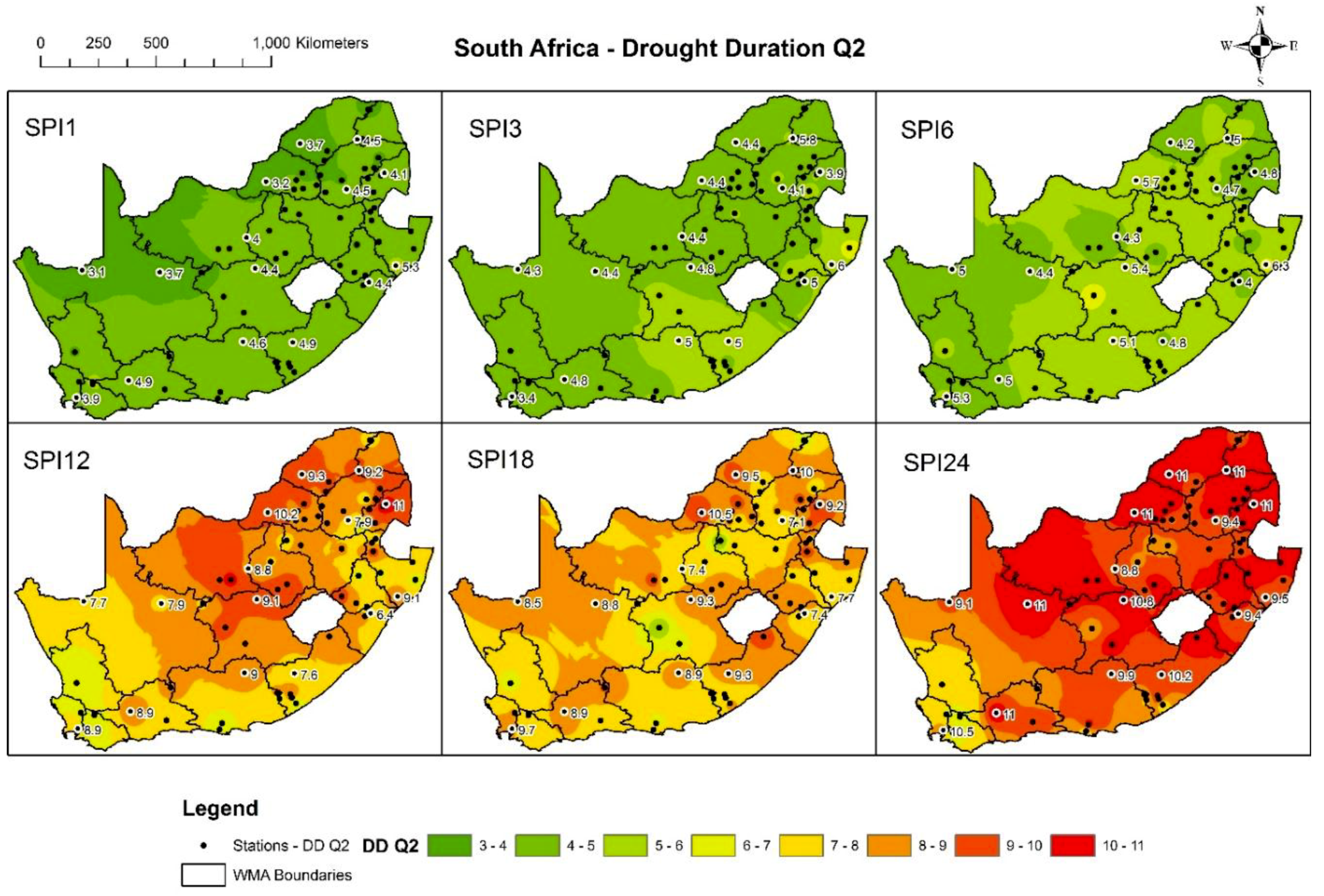
Given in Figure 4 is the 50th percentile of DD (hereafter Q2-DD) computed from the SPI-n. Analysis of the median values depicted in Figure 4 illustrates that the spatial variability of Q2-DD values across South Africa exhibit clear temporal dependence. The dependence structure has two main dominant accumulation time scale classes, i.e., n1 ≡ {1, 3, and 6} and n2 ≡ {12, 18, 24}. These accumulation time-scales correspond to meteorological-agricultural and hydrological drought phases, respectively. The Q2-DD values computed from SPI-1 accumulation time scale class delineate South Africa’s 19 WMAs into two dominant regions, i.e., one exhibiting Q2-DD < 4 and the other with 4 < Q2-DD < 6 months. As depicted in Figure 4 (top row), there exists a clear shift in the areal coverage of higher Q2-DD values with an increase in the accumulation period implying that large areas of South Africa gradually experience persistent drought conditions as a meteorological drought progresses to agricultural drought. The Q2-DD values derived from the SPI-2 accumulation time scale class delineate the WMAs into four regions with the following domains: 6 < Q2-DD < 7, 7 < Q2-DD < 8; 8 < Q2-DD < 9, and 9 < Q2-DD < 11. The distribution of Q2-DD values corresponding to SPI-1 and SPI-2 across the WMAs are given in Table 4.
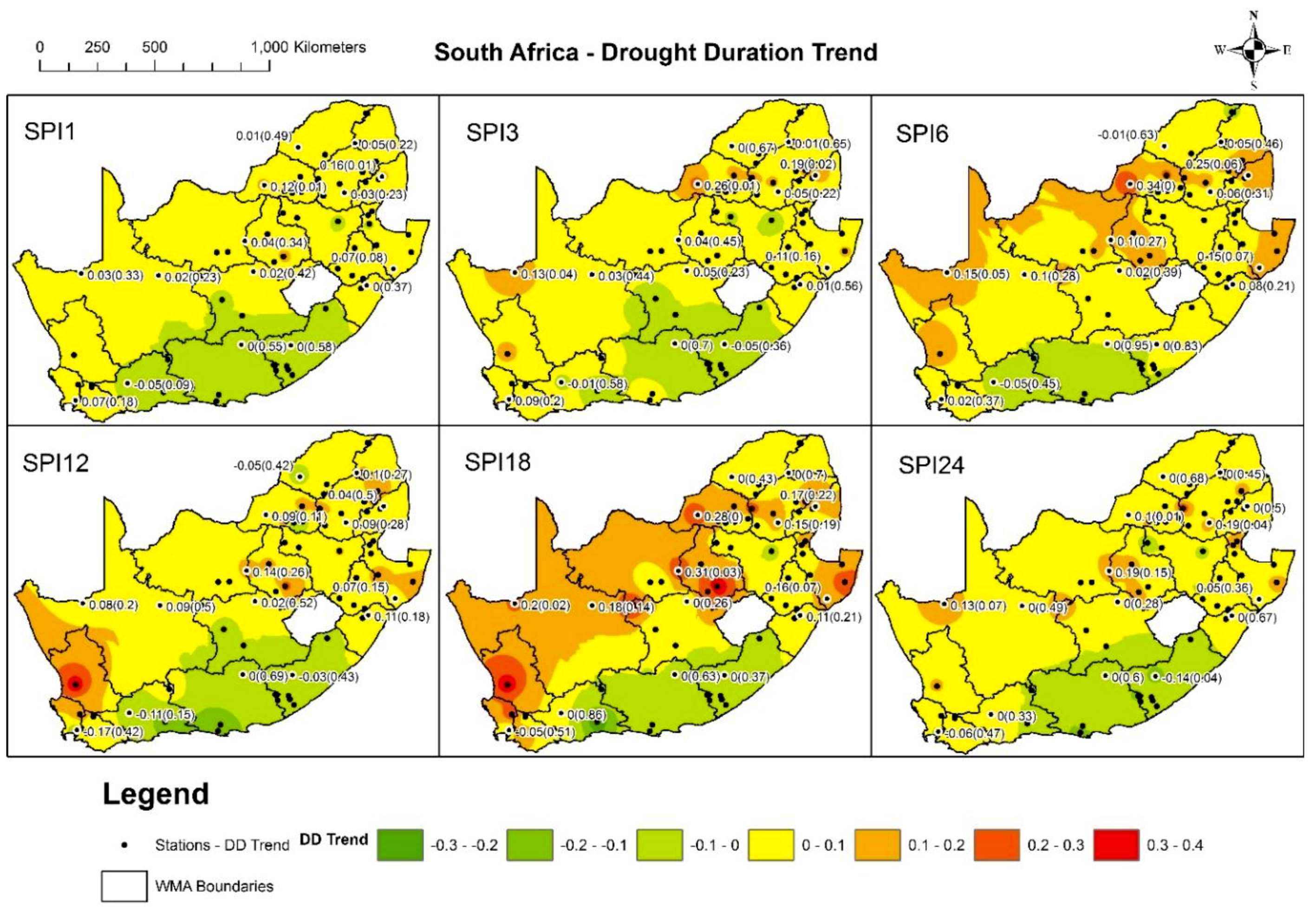
Spatial patterns of the temporal trends in DD derived from SPI-n {n ≡ 1, 3, 6, 12, 18 and 24} given in Figure 5 illustrate largely insignificant subtle positive trends (negative trends comprise of ~11% of the WMAs). As shown in Figure 5, the spatial distribution of DD trends derived from SPI-n {n ≡ 1, 3, and 24} delineate South Africa into two regions. In addition, those derived from SPI-n {n≡ 6, 12, and 18} exhibit largely negative temporal trends. Overall, the DD trends range from −0.3–0.4 months/year.
The DS for the 50th percentile (hereafter Q2-DS) given in Figure 6 illustrates that the Q2-DS exhibits spatial-temporal variability across the WMAs in South Africa. In particular, the Q2-DS for SPI-n (n ≡ {1 and 24}) delineates the WMAs into three dominant regions, i.e., 6 < Q2-DS < 10 (apparent in 11% and 58% WMAs for SPI-1 and SPI-24 respectively); 5 < Q2-Ds < 6 (present in 79% of WMAs for DS values derived from both SPI-1 and SPI-24), and 2 < Q2-DS < 5 (present in 68% of the WMAs). The Q2-DS derived from SPI-3 and SPI-6 have subtle spatial differences across the two time scales, yet illustrate that the WMAs could be delineated into two main regions characterized by the domains 2 < Q2-Ds < 4 (present in 58% of WMAs for DS values derived from both SPI-3 and SPI-6) and 4 < Q2-DS < 5 (present in 68% of the WMAs). Lastly, the Q2-DS computed from SPI-n (n ≡ {12 and 18}) exhibit higher regularity. That is, the Q2-DS derived from SPI-12 and SPI-18 depicts that the WMAs could be delineated into four regions with the domains 2 < Q2-DS < 4 (present in 53% of the WMAs); 4 < Q1-DS < 5 (dominant in most WMAs); 5 < Q2-DS < 6 and 6 < Q2-DS < 10 (quite localized in only 21% of the WMAs).
The spatiotemporal trends in DS corresponding to the SPI-n {n ≡ 1, 3, 6, 12, 18 and 24} over the 19 WMAs across South Africa (see Figure 7) demonstrate statistically insignificant trends ranging between −1.2–1.8 per year. Furthermore, there exists no apparent spatial variability inherent for the DS derived from SPI-1, SPI-3, and SPI-6 across all the WMAs. However, there exists some clustering tendency for DS trends derived from SPI-12, SPI-18, and SPI-24. In this regard, the variability patterns of the DS trends delineate the WMAs into three dominant regions, i.e., WMAs (present in less than 11% of the total WMAs) with trends less than −0.15 per year, WMAs exhibiting trends in the range of −0.15 and 0.2 per year, and WMAs with positive trends (which constitute about 32% of the WMAs) with magnitudes of 0.2 up to 1.6 per year.
3.2. Spatial Patterns of Drought Transition Periods
As mentioned in the methodology section, the drought propagation was assessed by cross-correlating SSI-1 with SPI accumulation periods from 1–24 months. For this analysis, two- (e.g., Gamma, Lognormal, and Gumbel) and three-parameter (Generalized Logistic and Tweedie) statistical distribution functions were considered. The results are illustrated in Figure 8, Figure 9 and Figure 10. In Figure 8, the top panel (A) depicts the two-parameter Gamma distribution analysis results, whereas results for two-parameter Lognormal distribution function analysis are depicted in the bottom panel (B). For the considered study period (1985–2016), the drought transition periods in South Africa can be grouped as follows: Shorter timescales covering 1–3 months, intermediate timescales covering 4–6 months, longer timescales that cover 7–12 months, and extended timescales which go beyond 12 months. Based on the Gamma distribution, regions exhibiting short-to-intermediate drought transition periods are found in parts of the Northern Cape, Eastern Cape, and some pocketed areas in the Free State Province. Overall, drought transition periods derived based on SPI computed with the Gamma distribution are apportioned across the WMAs as follows: About 16% of the WMAs have drought transition periods in the short timescale category, 37% exhibit intermediate drought transition periods, and long and extended drought transition periods are apparent in 47% and 63% of the WMAs, respectively. When considering drought transition periods derived from the Lognormal fitted SPI, the short-to-medium drought transition periods spread to parts of the Western Cape Province while diminishing in the Eastern Cape Province. The vast majority of South African regions (>60%) experience a delay in drought propagation (from one year up to 2 years). In particular, drought transition time scales in the short, intermediate, and longer time scales exist in 47%, 47%, and 53% of the WMAs, respectively, while the extended drought transition periods are experienced in 84% of the WMAs.
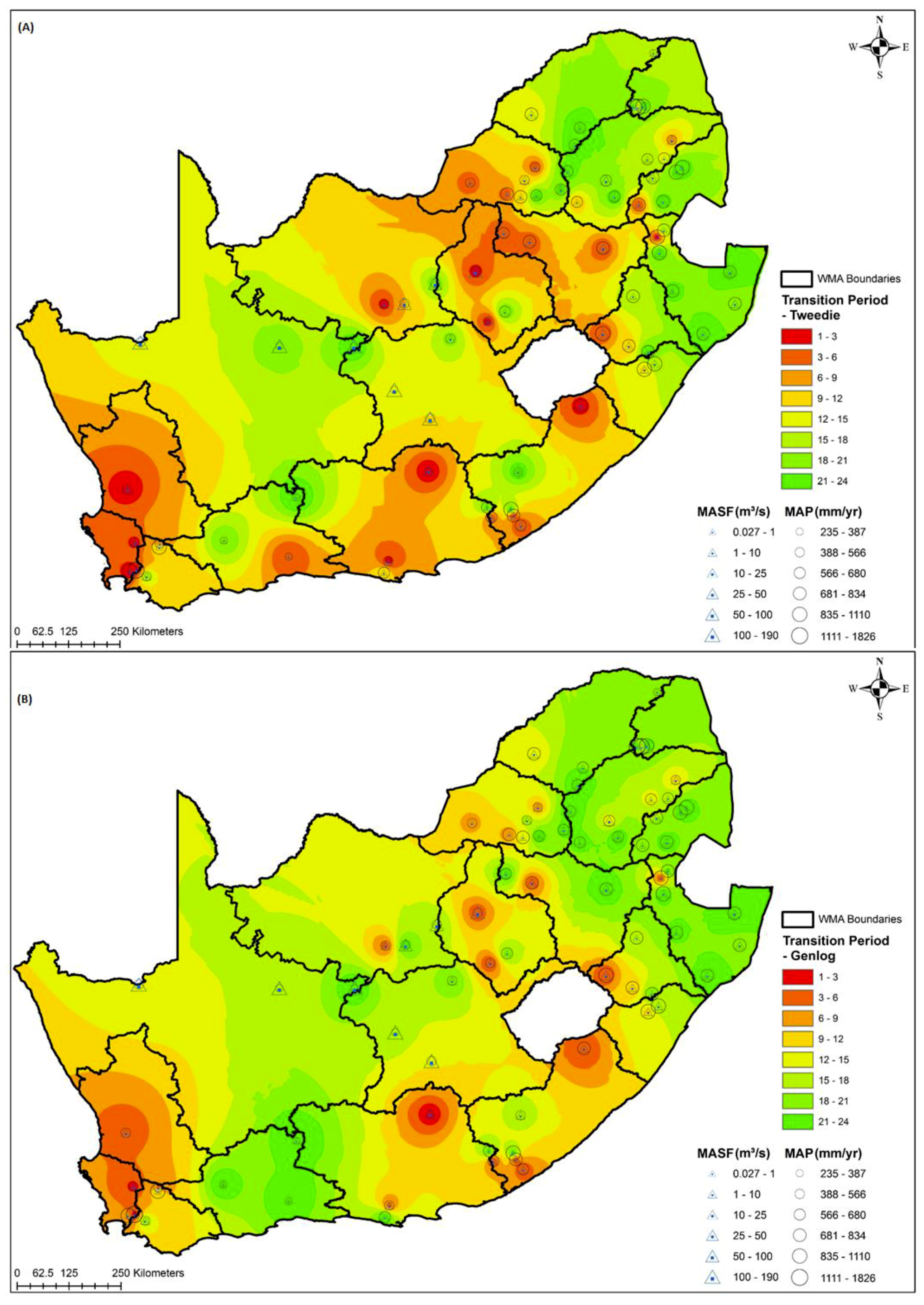
Figure 9A,B depicts the three-parameter Tweedie and the Generalized Logistic distribution functions analysis results, respectively. Based on the Tweedie distribution function, vast areas in the North West, Free State, Western Cape, Eastern Cape, and small areas in the KwaZulu-Natal Province exhibit short-to-intermediate drought transition periods. The rest of the regions show drought propagation periods ranging from long (12 months) to extended (up to 24 months) timescales. In this regard, about 47% and 53% of the WMAs exhibit short and intermediate drought transition periods, while long and extended drought transition periods comprise some parts of the 68% and 84% of the WMAs, respectively. On the other hand, the three-parameter Generalized Logistic analysis depicts a delay in the drought propagation time in most South African regions. The Western Cape Province and small pocket areas in the Eastern Cape, KwaZulu-Natal, and Free State provinces depict short-to-medium drought transition properties. This corresponds to 42%, 53%, 74%, and 79% of the WMAs with short, intermediate, long, and extended drought transition periods respectively.
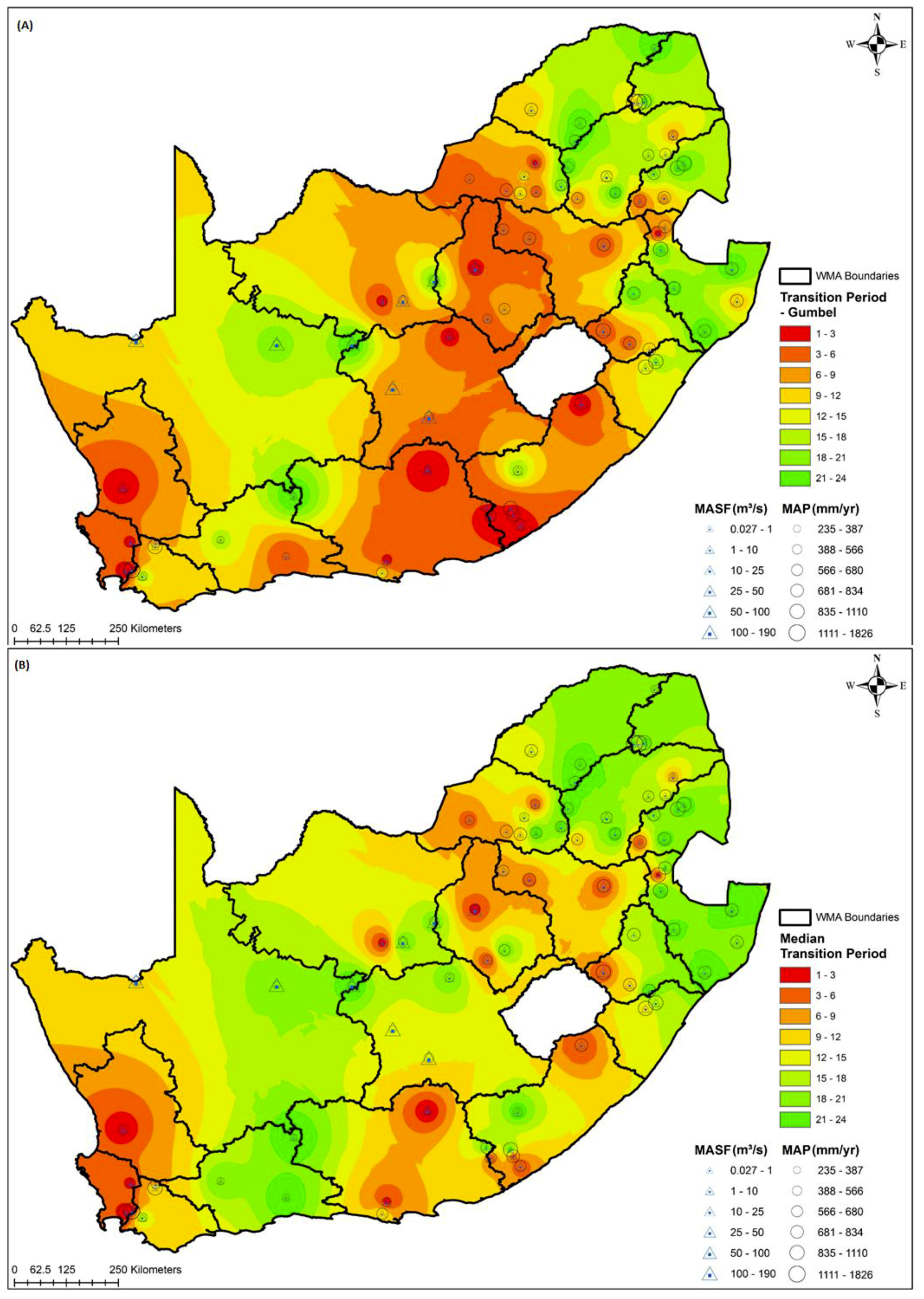
Figure 10A depicts results computed from the two-parameter Gumbel distribution function. There is a high variation of drought propagation timescales when the Gumbel distribution function is considered. In particular, results suggest that drought propagates quicker in six of the South African provinces, namely the Eastern Cape, Western Cape, KwaZulu-Natal, North West, Free State, and Gauteng, as well as in some regions in the Northern Cape Province. Delay in the drought transition period is observed mostly towards the Northeastern regions covering Limpopo, Mpumalanga, and KwaZulu-Natal, as well as in the Southwestern regions covering the Northern Cape Province. As depicted in Figure 10A, short and intermediate drought transition periods are in about 37% and 32% of the WMAs, while long to extended drought transition periods are apparent in 37% and 74% of the WMAs respectively. The spatial distributions of the median drought propagation period results are depicted in Figure 10B. The drought propagation patterns observed in Figure 10B are similar to those presented in Figure 8B and Figure 9B, with the Northeastern and central Southwestern regions depicting a high tendency of drought propagation delay. As shown in Figure 10B, 37% of the WMAs exhibit short and long drought propagation periods, while intermediate and extended drought propagation periods are characteristic in 32% and 74% of the WMAs, respectively.
3.3. Aggregating the Drought Transition Periods
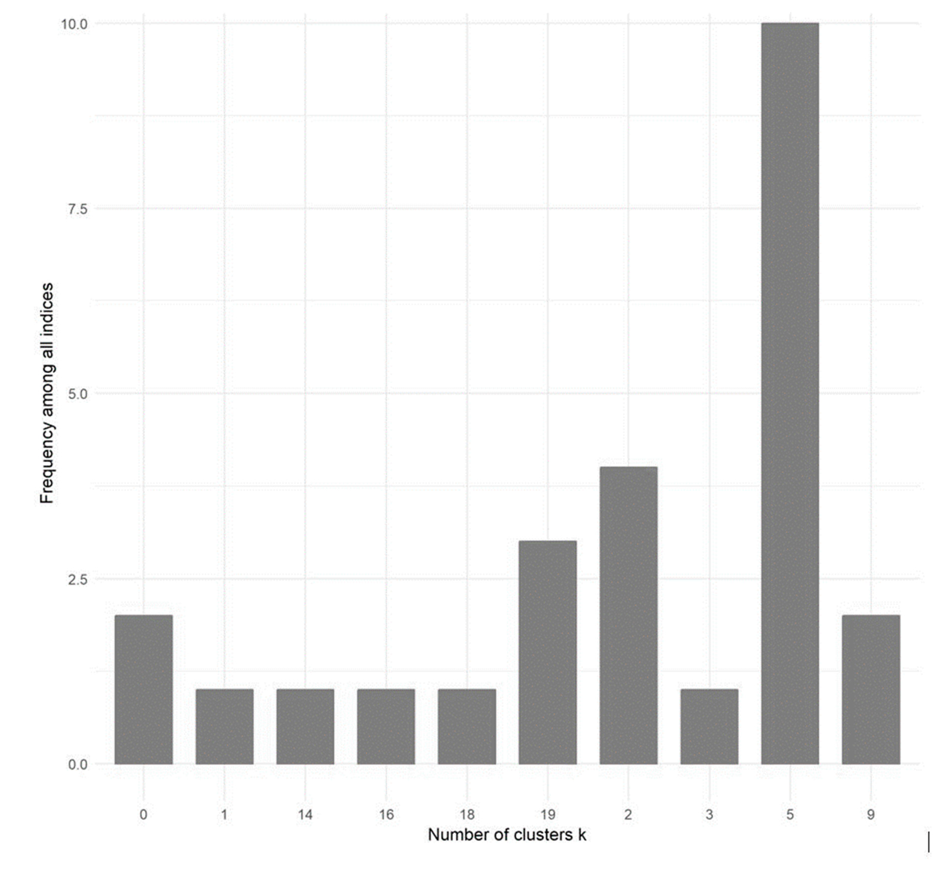
The aim of clustering drought transition periods was to delineate South African catchment areas into small zones that exhibit self-similar drought propagation timescales. In addition, other parameters which characterize the catchment hydrometeorology (including catchment area, drainage density of the catchment, MAP, and MASF) were incorporated during clustering in order to assess their influence on the spatial partitioning of drought conditions across South Africa. As described in Section 2.3.2, clustering proceeded with a clustering tendency assessment. A clustering tendency assessment was undertaken with and without catchment hydrometeorology datasets. As given in Table 5, the H > 0.5, suggesting that both datasets are significantly clusterable. Furthermore, as shown in Table 5 and Figure 11, the plausible optimal number (2 and 5) of clusters has been determined considering 30 indices and based on the majority rule reported in Reference [21].
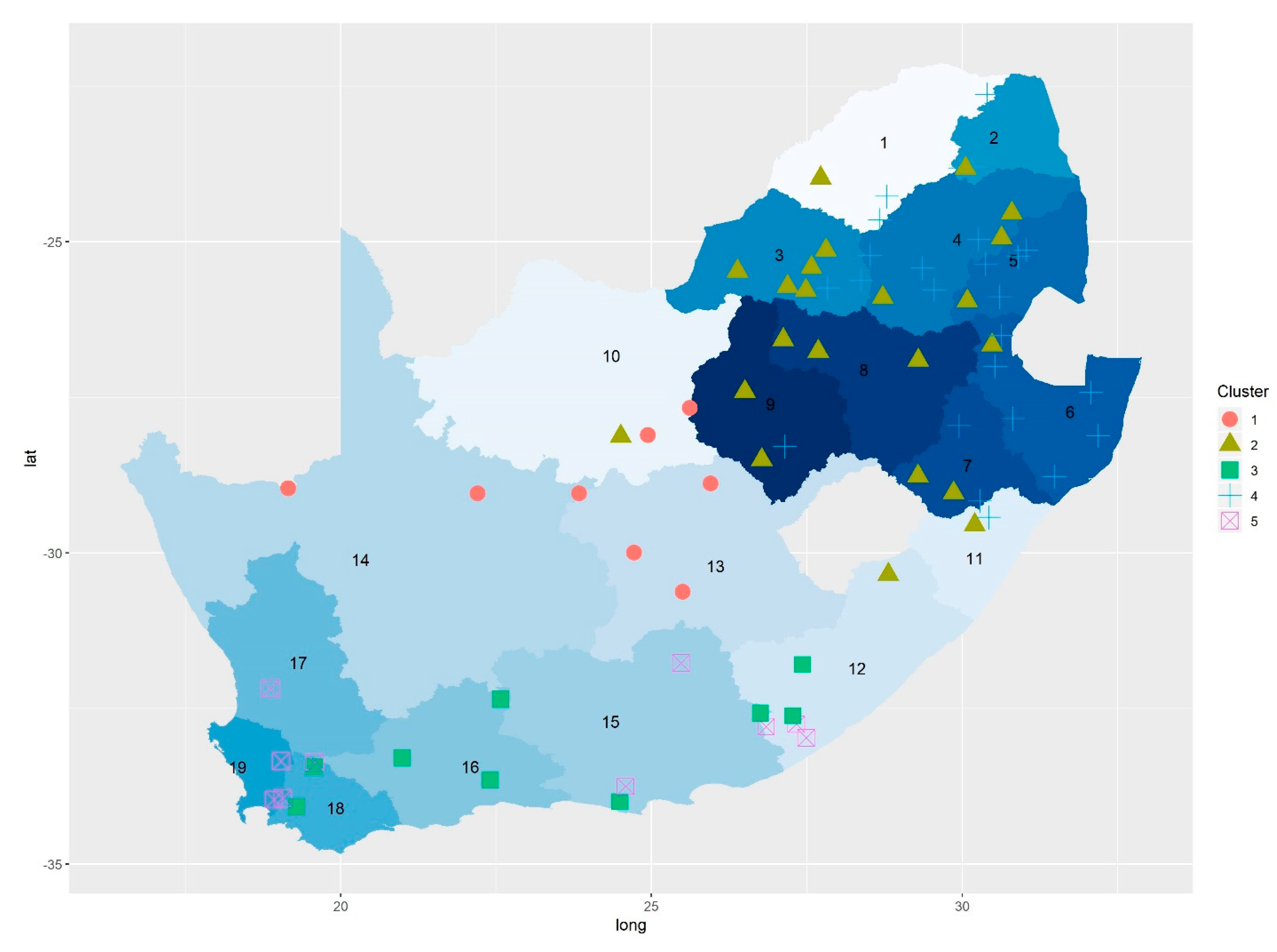
Figure 12 depicts the spatial grouping of zones of drought propagation timescales in all the WMAs across South Africa based on the K-means clustering. The K-means clustering was considered given that it is widely used and generally exhibits inherent scalability, efficiency, and simplicity (see References [24,25]). In order to evaluate the clustering results, internal validity indexes (i.e., the Dunn Index (DI) and Silhouette Coefficient (SC)) that often quantify the compactness and separability of the clusters were considered. From our results, the DI and SC values were determined as 0.2 and 0.3, respectively. These results illustrate that the apportionment of the clusters was plausible. As shown in Figure 12, WMAs over the Eastern and Northeastern parts of South Africa are dominated by clusters 2 and 4 (present in 63% and 53 % of the WMAs), the central interior regions of South Africa are largely dominated by cluster 1 (present in 16% of the WMAs), while the Western and Southwestern (coastal areas) are dominated by clusters 3 and 5, which are present in 21% and 26% of the WMAs, respectively.
4. Discussion
Drought undergoes different evolution stages as it progresses from the initial stage known as a meteorological drought. At each stage the drought reaches, it directly and indirectly affects different socioeconomic sectors, including water and agriculture. This study investigated the timescale over which a meteorological drought propagates to become a hydrological drought, where the impacts are on water resource management and planning. The results indicate that drought evolution across the 19 WMAs can be characterized by four main transition timescales, which are the short timescale covering 1–3 months, the intermediate covering 4–6 months, the long timescale that covers 7–12 months, and the extended time-scale which goes beyond 12 months. The WMAs found in arid to semi-arid areas (e.g., Olifants/Doorn Fish to Keiskamma, Lower Vaal) as well as in higher temperature regions (i.e., Crocodile West, Marico, Middle Vaal, Upper Vaal, and Mvoti to Umzimkulu areas) tend to lose water quicker either into the soil or through evapotranspiration, resulting in quicker transition periods. Extended (>12 months) drought propagation periods are observed mostly in the Northern as well as Northeastern regions, with biannual SPI accumulation periods strongly correlated with SSI-1.
Some parts of the Southwestern regions also depict a delay in drought propagation from meteorological to hydrological status. A delay in the propagation of drought in these regions could be attributed to seasonal rainfall, whereby the summer streamflow and water resources are highly dependent on winter recharge. In addition, most of the regions depicting long-to-extended propagation periods of drought are where major dams and aquifers are situated with water sources mainly being groundwater and surface water. This implies that the water reservoirs within these regions significantly influence the drought evolution. Other properties that may be influential to drought propagation characteristics include precipitation, catchment properties (e.g., the lowland/highland drainage, responsiveness), aquifer depth, the presence of lakes and wetlands, soil types, land cover/use, and climate change signals (see for example, References [7,28]). These catchment and climate characteristics have been used herein to demarcate spatial zones of drought propagation time scales throughout the WMAs. The clustering results point to five main clusters. Two clusters are concentrated in the Eastern parts of South Africa (comprised of the Limpopo, Mpumalanga, North-West, Gauteng and KZN provinces), one cluster is mainly concentrated in central interior (consisting of the Free State, Northern Cape and some parts of North-West Province) and Northwestern parts of South Africa, while two clusters dominate in the Western and coastal areas of South Africa (mainly in the Western Cape and Eastern Cape provinces). Overall, the resulting spatial drought transition zones subtly correspond to the broader climatic zones of South Africa, i.e., the Savanna, Grassland, Karoo, Fynbos, Forest and Desert zones [29].
5. Conclusions
A broader understanding of drought impact in South Africa can only be possible if the drought properties, i.e., drought duration, frequency, severity, and intensity, are jointly modeled (e.g., using multivariate techniques) and their inherent spatial-temporal dependence structure investigated. More importantly, it is necessary to have a consistent characterization of drought across the hydrological cycle. To be precise, analysis of drought propagation mechanisms in the hydrological cycle across the 19 WMAs of South Africa could be an important ingredient required for the design of robust drought monitoring and early warning systems (DM and EWS) vital for drought preparedness. We contributed to this noble cause by calculating the DD and DS of the drought events identified based on the SPI-n and SSI-1 across all the 19 South African WMAs. To this end, we assessed the spatial-temporal structure of drought characteristics across South Africa, and for the first time, examined the evolution of drought from meteorological to hydrological drought through cross-correlation of SSI-1 and SPI-n across the WMAs. Our methodology of spatial-temporal analysis and characterization of drought propagation across 19 MWAs in South Africa pointed us to the following main findings:
- (a)
- Averaged over three decades, drought conditions across the WMAs in South Africa exhibited a generally noticeable spatial-temporal dependence structure. This space-time proximity is dependent on common covariates illustrated by the spatial-temporal variability of quartiles, statistical moments and trends.
- (b)
- Drought propagation in South Africa is generally omnipresent. These transition periods exhibited four main transition timescales; (1) 1–3 months (hereafter short timescale), (2) the intermediate timescale which lasts approximately 4–6 months, (3) the long timescale which lasts between 7 and 12 months, and (4) the extended timescale which persists beyond 12 months.
- (c)
- Drought propagation evolution in South Africa is influenced by both catchment and climate characteristics. This conclusion arises from the spatial zones of drought propagation timescales throughout the WMAs, delineated using the climate and catchment characteristics through clustering.
- (d)
- It is worth noting that the resulting spatial drought transition zones (as elucidated in finding (c)) subtly correspond to the broader climatic zones of South Africa, i.e., Savanna, Grassland, Karoo, Fynbos, Forest, and Desert zones. These results underpin the current ongoing research on the role of climate characteristics on drought evolution in South Africa
In conclusion, we posit that the results from this study provide a new perspective on drought characterization in South Africa and could be of use to water resources planning strategies in support of drought preparedness. Furthermore, studies on drought evolution in the hydrological cycle in South Africa are expected to elicit further research on more complex topics such as drought termination typology. These studies are highly needed yet are still underdeveloped, especially in Southern Africa and Africa generally.
Author Contributions
Conceptualization, J.O.B. and C.M.B.; Methodology, J.O.B.; Software, J.O.B., A.M.A.; Validation, C.M.B., M.M., and A.M.A.; Formal Analysis, J.O.B.; Resources, J.O.B.; Data Curation, J.P.d.W.; Writing—Original Draft Preparation, J.O.B. and C.M.B.; Writing—Review and Editing, All; Visualization, J.O.B. and J.P.d.W.; Funding Acquisition, J.O.B.
Funding
This research was partly funded by the Water Research Commission project, grant number [K5/2309].
Acknowledgments
This study was carried out as part of the program of action spelt in the joint research collaboration between the South African Weather Service and the Central University of Technology, Free State, South Africa. We could like to thank the Department of Water and Sanitation (DWS), South Africa, for providing the analyzed precipitation and streamflow data. The authors could like to thank the anonymous reviewers whose valuable feedback help improve the manuscript.
Conflicts of Interest
The authors declare no conflict of interest.
References
- Tallaksen, L.M.; Van Lanen, A.A.J. Hydrological Drought: Processes and Estimation Methods for Streamflow and Groundwater; Elsevier: New York, NY, USA, 2004; Volume 48. [Google Scholar]
- Wang, W.; Ertsen, M.W.; Svoboda, M.D.; Hafeez, M. Propagation of drought: from meteorological drought to agricultural and hydrological drought. Adv. Meteorol. 2016. [Google Scholar] [CrossRef]
- Glickman, T.S. Glossary of Meteorology; American Meteorological Society: Boston, MA, USA, 2000; p. 855. [Google Scholar]
- Wilhite, D.A. (Ed.) Drought: A Global Assessment; Routledge: London, UK, 2000. [Google Scholar]
- Hisdal, H.; Stahl, K.; Tallaksen, L.M.; Demuth, S. Have streamflow drought in Europe become more severe or frequent? Int. J. Climatol. 2001, 21, 317–333. [Google Scholar] [CrossRef]
- Van Lanen, H.A.J.; Peters, E. Definition, effects and assessment of groundwater droughts. In Drought and Drought Mitigation in Europe; Vogt, J.V., Somma, F., Eds.; Kluwer Academic Publishers: Dordrecht, The Netherlands, 2000; pp. 49–61. [Google Scholar]
- Van Loon, A.F.; Laaha, G. Hydrological drought severity explained by climate and catchment characteristics. J. Hydrol. 2015, 526, 3–14. [Google Scholar] [CrossRef] [Green Version]
- Tallaksen, L.M.; Hisdal, H.; Van Lanen, H.A.J. Propagation of drought in a groundwater fed catchment, the Pang in the UK. Climate Variability and Change–Hydrological Impacts. In Proceedings of the Fifth FRIEND World Conference, Havana, Cuba, 27 November–1 December 2006; Volume 308. [Google Scholar]
- Eltahir, E.A.B.; Yeh, P.J.F. On the asymmetric response of aquifer water level to floods and droughts in IIIinois. Water Resour. Res. 1999, 35, 1199–1217. [Google Scholar] [CrossRef]
- White, I.; Falkland, T.; Scott, D. Droughts in Small Coral Islands: Case Study, South Tarawa, Kiribati; Technical Documents in Hydrology; Unesco: Paris, France, 1999; Volume 26. [Google Scholar]
- Price, M.; Low, R.G.; McCann, C. Mechanisms of water storage and flow in the unsaturated zone of the chalk aquifer. J. Hydrol. 2000, 233, 54–71. [Google Scholar] [CrossRef]
- Peters, E.; Van Lanen, H.A.J. Propagation of drought in groundwater in semi-arid and sub-humid climatic regimes. In Proceedings of the Hydrology of the Mediterranean and Semi-Adid Regions, Montpellier, France, 1–4 April 2003; Volume 278, pp. 312–317. [Google Scholar]
- Peters, E.; Torfs, P.J.J.F.; Van Lanen, H.A.J.; Bier, G. Propagation of drought through groundwater—A new approach using linear reservoir theory. Hydrol. Process. 2003, 17, 3023–3040. [Google Scholar]
- Peters, E.; Bier, G.; Van Lanen, H.A.J.; Torfs, P.J.J.F. Propagation and spatial distribution of drought in a groundwater catchment. J. Hydrol. 2006, 321, 257–275. [Google Scholar] [CrossRef]
- McKee, T.B.; Doesken, N.J.; Kleist, J. The relationship of drought frequency and duration of time scales. In Proceedings of the Eighth Conference on Applied Climatology, American Meteorological Society, Anaheim, CA, USA, 17–23 January 1993; pp. 179–186. [Google Scholar]
- Edwards, D.C.; McKee, T.B. Characteristics of 20th Century Drought in the United States at Multiple Time Scales; Climatology Report No. 97-2; Colorado State University: Collins, CO, USA, 1997. [Google Scholar]
- Guttman, N.B. Accepting the Standardized Precipitation Index: A calculation algorithm. J. Am. Water Resour. Assoc. 1999, 35, 311–322. [Google Scholar] [CrossRef]
- Stagge, J.H.; Tallaksen, L.M.; Gudmundsson, L.; Van Loon, A.F.; Stahl, K.; Barker, L.J.; Hannaford, J.; Chiverton, A.; Svensson, C. Candidate distributions for climatological drought indices (SPI and SPEI). Int. J. Climatol. 2015, 35, 4027–4040. [Google Scholar] [CrossRef]
- Barker, L.J.; Hannaford, J.; Chiverton, A.; Svensson, C. From meteorological to hydrological drought using standardized indicators. Hydrol. Earth Syst. Sci. 2016, 20, 2483–2505. [Google Scholar] [CrossRef]
- Banerjee, A.; Dave, R.N. Validating clusters using the Hopkins statistic. In Proceedings of the 2004 IEEE Conference on Fuzzy Systems (FUZZ-IEEE 2004), Budapest, Hungary, 25–29 July 2004; pp. 149–153. [Google Scholar]
- Charrad, M.; Ghazzali, N.; Boiteau, V.; Niknafs, A. NbClust: An R Package for Determining the Relevant Number of Clusters in a Data Set. J. Stat. Softw. 2014, 61, 1–36. [Google Scholar] [CrossRef]
- Liu, Y.; Li, Z.; Xiong, H.; Gao, X.; Wu, J. Understanding of Internal Clustering Validation Measures. In Proceedings of the 2010 IEEE International Conference on Data Mining (ICDM ‘10), Sydney, Australia, 13–17 December 2010; pp. 911–916. [Google Scholar]
- Brock, G.; Vasyl, P.; Susmita, D.; Somnath, D. ClValid: An R Package for Cluster Validation. J. Stat. Softw. 2008, 25, 1–22. [Google Scholar] [CrossRef]
- Nawrin, S.; Rahman, M.R.; Akhter, S. Exploring K-means with internal validity indexes for data clustering in traffic management system. Int. J. Adv. Comput. Sci. Appl. 2017, 8, 264–272. [Google Scholar]
- Zhang, J.; Wu, W.; Hu, X.; Li, S.; Hao, S. A Parallel Clustering Algorithm with MPI-MKmeans. J. Comput. 2013, 8, 10–17. [Google Scholar] [CrossRef]
- Kapil, S.; Chawla, M. Performance evaluation of k-means clustering algorithm with various distance metrics. In Proceedings of the IEEE 1st International Conference on Power Electronics, Intelligent Control and Energy Systems, Delhi, India, 4–6 July 2016; pp. 1–4. [Google Scholar]
- Chen, H.; Fan, L.; Wu, W.; Liu, H.B. Comparison of spatial interpolation methods for soil moisture and its application for monitoring drought. Environ. Monit. Assess. 2017, 189, 525–541. [Google Scholar] [CrossRef] [PubMed]
- Ali, M.G.; Younes, K.; Esmaeil, A.; Fatemeh, T. Assessment of geostatistical methods for spatial analysis of SPI and EDI drought indices. World Appl. Sci. J. 2011, 15, 474–482. [Google Scholar]
- Apurv, T.; Sivapalan, M.; Cai, X. Understanding the role of climate characteristics in drought propagation. Water Resour. Res. 2017, 53, 9304–9329. [Google Scholar] [CrossRef]
Figure 1.
A map depicting the study area. The selected rainfall and streamflow stations are fairly distributed across all the 19 Water Management Areas (WMA) across South Africa. The map also depicts the mean annual precipitation and mean annual streamflow as recorded at the selected stations.
Figure 1.
A map depicting the study area. The selected rainfall and streamflow stations are fairly distributed across all the 19 Water Management Areas (WMA) across South Africa. The map also depicts the mean annual precipitation and mean annual streamflow as recorded at the selected stations.

Figure 2.
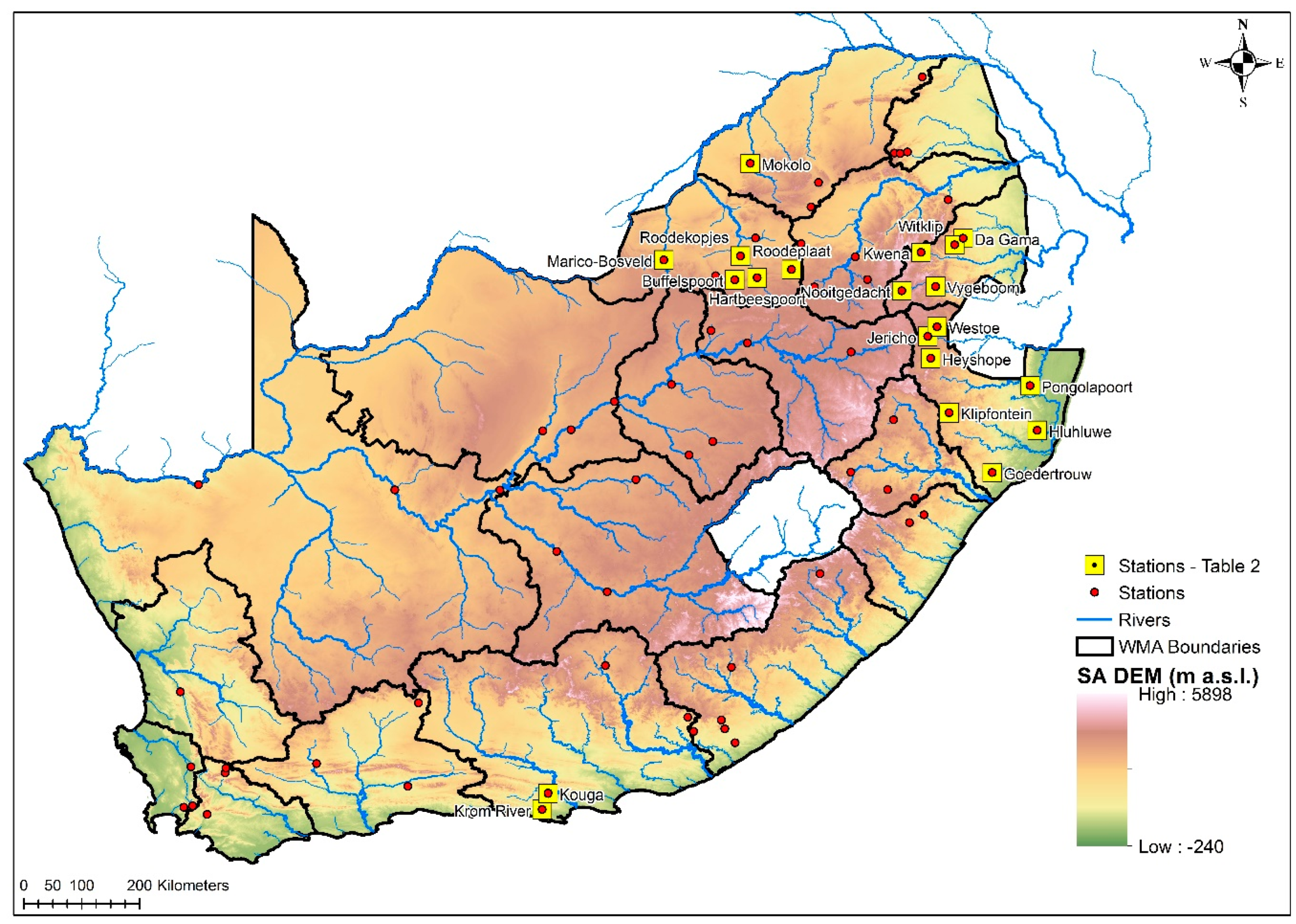
A map showing the location of some of the stations with rainfall, streamflow characteristics, and elevation in meters above sea level given in Table 2 (see legend).
Figure 2.
A map showing the location of some of the stations with rainfall, streamflow characteristics, and elevation in meters above sea level given in Table 2 (see legend).

Figure 3.
The schema used for drought characterization across South Africa. A total of k (i.e., k = 1, 2, …, 5) probability distribution functions (PDF) comprised of the two- and three-parameter probability distributions were considered.
Figure 3.
The schema used for drought characterization across South Africa. A total of k (i.e., k = 1, 2, …, 5) probability distribution functions (PDF) comprised of the two- and three-parameter probability distributions were considered.

Figure 4.
Spatial-temporal distribution of the 50th percentile of drought duration derived from SPI-1, SPI-3, SPI-6, SPI-12, SPI-18, and SPI-24 accumulation periods.
Figure 4.
Spatial-temporal distribution of the 50th percentile of drought duration derived from SPI-1, SPI-3, SPI-6, SPI-12, SPI-18, and SPI-24 accumulation periods.

Figure 5.
Trends in drought duration derived from SPI-1, SPI-3, SPI-6, SPI-12, SPI-18, and SPI-24 accumulation periods. The significance levels are given in brackets.
Figure 5.
Trends in drought duration derived from SPI-1, SPI-3, SPI-6, SPI-12, SPI-18, and SPI-24 accumulation periods. The significance levels are given in brackets.

Figure 6.
This figure is the same as Figure 4 but it illustrates drought severity.
Figure 6.
This figure is the same as Figure 4 but it illustrates drought severity.

Figure 7.
Spatial patterns of temporal trends in drought severity derived from SPI-1, SPI-3, SPI-6, SPI-12, SPI-18, and SPI-24 accumulation periods. The significance levels are given in brackets.
Figure 7.
Spatial patterns of temporal trends in drought severity derived from SPI-1, SPI-3, SPI-6, SPI-12, SPI-18, and SPI-24 accumulation periods. The significance levels are given in brackets.

Figure 8.
The drought transition period from meteorological to hydrological drought calculated using two-parameter statistical distribution functions (A) Gamma and (B) Lognormal.
Figure 8.
The drought transition period from meteorological to hydrological drought calculated using two-parameter statistical distribution functions (A) Gamma and (B) Lognormal.

Figure 9.
The drought transition period from meteorological to hydrological calculated using the three-parameter statistical distribution functions: (A) Tweedie and (B) Generalized Logistic.
Figure 9.
The drought transition period from meteorological to hydrological calculated using the three-parameter statistical distribution functions: (A) Tweedie and (B) Generalized Logistic.

Figure 10.
The drought transition period from meteorological to hydrological calculated using the two-parameter statistical distribution functions (A) Gumbel and (B) the average of the five selected statistical distribution functions.
Figure 10.
The drought transition period from meteorological to hydrological calculated using the two-parameter statistical distribution functions (A) Gumbel and (B) the average of the five selected statistical distribution functions.

Figure 11.
The optimal number of clusters.

Figure 12.
Spatial dependence of drought conditions based on K-means clustering. The underlying colors depict the different WMAs (denoted by the different).
Figure 12.
Spatial dependence of drought conditions based on K-means clustering. The underlying colors depict the different WMAs (denoted by the different).


Table 1.
Summary of some of the physiographic characteristics of Water Management Areas in South Africa. These physiographic characteristics refer to buffer zone (10 km radius) area characteristics averaged across the selected rainfall and streamflow stations within the Water Management Areas.
Table 1.
Summary of some of the physiographic characteristics of Water Management Areas in South Africa. These physiographic characteristics refer to buffer zone (10 km radius) area characteristics averaged across the selected rainfall and streamflow stations within the Water Management Areas.
| Some WMAs (Code, See Figure 1) | Mean Altitude above Sea Level (m a.s.l) | Dominant Land Cover | Dominant Soil Texture | Soil Bulk Density |
|---|---|---|---|---|
| 1 | 1021.31 | Woodlands/Open Bush | Loam; Clay Loam; Sandy Clay Loam | 1.38 |
| 6 | 876.34 | Thicket/Dense Bush; Plantations/Woodlots; Grasslands | Clay; Clay Loam; Sandy Loam; Sandy Clay Loam | 1.39 |
| 9 | 1343.74 | Grasslands; Cultivated Commercial Annual Crops Non-Pivot | Clay Loam; Sandy Clay Loam | 1.42 |
| 10 | 1169.25 | Grassland; Low Shrub land | Clay; Sandy Loam | 1.34 |
| 14 | 853.54 | Low shrub land; Nama Karoo: Low Shrub; Bare ground | Clay Loam | 1.31 |
| 15 | 640.04 | Thicket/Dense bush; Fynbos: Low shrub; Nama Karoo: Low Shrub | Clay; Clay Loam | 1.33 |
| 18 | 859.42 | Fynbos: Low shrub | Loam; Clay Loam | 1.32 |
| 19 | 397.02 | Cultivated Commercial Annual Crops Non-Pivot; Fynbos: Low shrub | Clay Loam; Sandy Loam | 1.44 |
Table 2.
Rainfall and streamflow characteristics of some of the stations considered in the study.
| Location | Latitude (Degrees) | Longitude (Degrees) | Catchment Area (km2) | Data Records | MASF (m3/s) | MAP (mm/Year) |
|---|---|---|---|---|---|---|
| Hartbeespoort Dam | −25.7485 | 27.8323 | 4116 | 11688 | 0.525 | 655 |
| Buffelspoort Dam | −25.7797 | 27.4853 | 88 | 11684 | 0.300 | 733 |
| Roodeplaat Dam | −25.6205 | 28.3675 | 685 | 11688 | 1.378 | 681 |
| Roodekopjes Dam | −25.4109 | 27.5719 | 6131 | 11111 | 7.320 | 558 |
| Marico-Bosveld Dam | −25.4718 | 26.3818 | 1220 | 11656 | 0.501 | 496 |
| Mokolo Dam | −23.9733 | 27.7240 | 4319 | 11323 | 4.050 | 722 |
| Krom River Dam | −33.9991 | 24.4936 | 368.5 | 11688 | 0.631 | 654 |
| Kouga Dam | −33.7492 | 24.5862 | 29,560 | 11688 | 2.079 | 435 |
| Goedertrouw Dam | −28.7740 | 31.4822 | 1273 | 11657 | 3.289 | 696 |
| Klipfontein Dam | −27.8415 | 30.8156 | 341 | 11658 | 0.947 | 786 |
| Hluhluwe Dam | −28.1171 | 32.1831 | 734 | 11628 | 1.434 | 739 |
| Pongolapoort Dam | −27.4237 | 32.0709 | 7831 | 11537 | 18.156 | 707 |
| Jericho Dam | −26.6586 | 30.4805 | 218 | 11688 | 0.077 | 866 |
| Westoe Dam | −26.5090 | 30.6256 | 531 | 11688 | 0.450 | 834 |
| Heyshope Dam | −26.9990 | 30.5281 | 1122 | 11686 | 2.597 | 859 |
| Nooitgedacht Dam | −25.9505 | 30.0789 | 1570 | 11688 | 0.575 | 733 |
| Vygeboom Dam | −25.8839 | 30.6039 | 3112 | 11688 | 4.838 | 800 |
| Witklip Dam | −25.2381 | 30.8997 | 64 | 11688 | 0.463 | 1110 |
| Kwena Dam | −25.3547 | 30.3789 | 947 | 11688 | 3.624 | 698 |
| Da Gama Dam | −25.1339 | 31.0331 | 62 | 11381 | 0.354 | 1071 |
Table 3.
Two- and three-parameter statistical probability distributions considered in the study.
| Probability Distribution Function (Parameter) | Parametric Distribution |
|---|---|
| Gamma (two-) | for x > 0; where is the gamma function |
| Log-normal (two-) | ; ; where μ and are the mean and standard deviation of the logarithmically transformed variables, respectively. |
| Gumbel(two-) | , ; where k > 0 is the shape parameter |
| Generalized logistic (three-) | ; where and , k = 0 |
| Tweedie (three-) | where μ is the mean of the distribution, > 0 and a are unknown functions and θ and κ(θ) are known functions |
Table 4.
Distribution of Q2-DD domains across WMAs.
| SPI-n | Q2-DD Values (Months) | WMAs Dominated (Code) | Proportion (%) of WMA with ~ ≥ 50% DD Areal Coverage | |
|---|---|---|---|---|
| SPI-n1 | 1 | <3 | 1, 3, 4, 10, 14 | 26.3 |
| 3< Q2-DD < 4 | 1, 2, 4, 5, 6, 8, 9, 10, 11, 12, 13, 14, 15, 16, 17, 18, 19 | 89.5 | ||
| 3 | <4 | All except 12, 13, 15 | 84.2 | |
| 4 < Q2-DD < 6 | 6, 7, 11, 12, 13, 15 | 31.6 | ||
| 6 | <4 | 1, 2, 3, 5, 14, 17, 18, 19 | 42.1 | |
| 4 < Q2-DD < 7 | All except 1, 14, 17, 18, 19 | 26.3 | ||
| SPI-n2 | 12 | 6 < Q2-DD < 7 | 17,18 | 10.5 |
| 7 < Q2-DD < 8 | 6, 7, 12, 14,15,16 | 31.6 | ||
| 8 < Q2-DD < 9 | 1, 2, 4, 8, 9, 13, 14 | 36.8 | ||
| 9 < Q2-DD < 11 | 1, 3, 5, 10 | 21.1 | ||
| 18 | 5 < Q2-DD < 7 | 13 | 5.3 | |
| 7 < Q2-DD < 8 | 4, 8, 9, 12, 13, 17 | 31.6 | ||
| 8 < Q2-DD < 9 | 1, 2, 3, 4, 5, 10, 11, 14, 15 | 47.4 | ||
| 9 < Q2-DD < 11 | 1,3 | 10.5 | ||
| 24 | 6 < Q2-DD < 7 | 18 | 5.3 | |
| 7 < Q2-DD < 8 | 17, 18, 19 | 15.8 | ||
| 8 < Q2-DD < 9 | 14 | 1.0 | ||
| 9 < Q2-DD < 11 | All except 17, 18, 19 | 84.5 | ||
Table 5.
Clustering tendency statistic.
| Catchment Characteristic | H-Statistic | Maximum Number of Cluster (Sizes) | Remarks |
|---|---|---|---|
| No catchment hydrometeorology | 0.69 | 2 (43, 31) | Only drought propagation months for the various probability distributions are considered. The data sets are generally clusterable. |
| Catchment hydrometeorology present | 0.71 | 5 (25, 9, 22, 10, 8) | Data set is clusterable. |
© 2019 by the authors. Licensee MDPI, Basel, Switzerland. This article is an open access article distributed under the terms and conditions of the Creative Commons Attribution (CC BY) license (http://creativecommons.org/licenses/by/4.0/).
Share and Cite
MDPI and ACS Style
Botai, J.O.; Botai, C.M.; de Wit, J.P.; Muthoni, M.; Adeola, A.M. Analysis of Drought Progression Physiognomies in South Africa. Water 2019, 11, 299. https://doi.org/10.3390/w11020299
AMA Style
Botai JO, Botai CM, de Wit JP, Muthoni M, Adeola AM. Analysis of Drought Progression Physiognomies in South Africa. Water. 2019; 11(2):299. https://doi.org/10.3390/w11020299
Chicago/Turabian StyleBotai, Joel Ondego, Christina M. Botai, Jaco P. de Wit, Masinde Muthoni, and Abiodun M. Adeola. 2019. "Analysis of Drought Progression Physiognomies in South Africa" Water 11, no. 2: 299. https://doi.org/10.3390/w11020299
Note that from the first issue of 2016, this journal uses article numbers instead of page numbers. See further details here.