Real-Time Urban Inundation Prediction Combining Hydraulic and Probabilistic Methods


1
Department of Civil Engineering, Kyungpook National University, 80 Daehak-ro, Buk-gu Daegu 41566, Korea
2
Disaster Prevention Research Institute, Kyungpook National University, 80 Daehak-ro, Buk-gu Daegu 41566, Korea
*
Author to whom correspondence should be addressed.
Water 2019, 11(2), 293; https://doi.org/10.3390/w11020293
Submission received: 24 December 2018
/
Revised: 24 January 2019
/
Accepted: 31 January 2019
/
Published: 8 February 2019
(This article belongs to the Special Issue Urban Rainfall Analysis and Flood Management)
Abstract
:Damage caused by flash floods is increasing due to urbanization and climate change, thus it is important to recognize floods in advance. The current physical hydraulic runoff model has been used to predict inundation in urban areas. Even though the physical calculation process is astute and elaborate, it has several shortcomings in regard to real-time flood prediction. The physical model requires various data, such as rainfall, hydrological parameters, and one-/two-dimensional (1D/2D) urban flood simulations. In addition, it is difficult to secure lead time because of the considerable simulation time required. This study presents an immediate solution to these problems by combining hydraulic and probabilistic methods. The accumulative overflows from manholes and an inundation map were predicted within the study area. That is, the method for predicting manhole overflows and an inundation map from rainfall in an urban area is proposed based on results from hydraulic simulations and uncertainty analysis. The Second Verification Algorithm of Nonlinear Auto-Regressive with eXogenous inputs (SVNARX) model is used to learn the relationship between rainfall and overflow, which is calculated from the U.S. Environmental Protection Agency’s Storm Water Management Model (SWMM). In addition, a Self-Organizing Feature Map (SOFM) is used to suggest the proper inundation area by clustering inundation maps from a 2D flood simulation model based on manhole overflow from SWMM. The results from two artificial neural networks (SVNARX and SOFM) were estimated in parallel and interpolated to provide prediction in a short period of time. Real-time flood prediction with the hydraulic and probabilistic models suggested in this study improves the accuracy of the predicted flood inundation map and secures lead time. Through the presented method, the goodness of fit of the inundation area reached 80.4% compared with the verified 2D inundation model.
1. Introduction
Flooding in urban areas has caused not only human casualties and property damage, but also social, environmental, economic, and psychological damage. It also causes damage to urban infrastructure, such as roads and subways, as well as critical utilities including electricity, gas, and water supply. This is followed by paralysis of urban functions and collapse of the social system. Inundation in urban areas occurs due to a lack of flow conveyance by pipes during heavy rainfall [1]. Flood damage in metropolitan cities arises due to insufficient capacity of sewer pipes and drainage facilities, rather than by river inundation [2].
In the Gangnam area of Korea, two major flooding events occurred on 21 September 2010 (98.5 mm/h, 233 mm/3 h), and 27 July 2011 (113 mm/h, 218.5 mm/3 h), in which torrential rains of more than approximately 100 mm/h poured, causing serious damage. Studies on floods are actively performed; however rainfall runoff simulations with existing hydrologic/hydraulic models for flood prediction cannot secure sufficient lead time due to the long simulation times required. In addition, the existing model does not provide the ability to analyze each sewer pipe in an urban area with the promptness required to secure sufficient lead time. Two-dimensional (2D) flood simulations that display an inundation area take a long time. Thus, it is difficult to conduct flood analysis in real time for predicting inundation by using only existing 1D/2D simulation programs [3,4].
A large number of studies have focused on flood prediction, and they have generally used rainfall–runoff analysis and 2D hydraulic analysis models to estimate runoff patterns in urban areas. Artificial neural network (ANN), genetic algorithm, or neuro-fuzzy models are also used to predict floods. In water resource engineering, ANNs have been successfully used for simulating rainfall–runoff [5,6,7], flood and short-term rainfall predictions [8,9], and hydrological factor analysis and prediction [10,11]. In addition, Chang et al. [12] developed a hybrid flood prediction system based on a clustering technique using a backpropagation neural network (BPNN). Pan et al. [13] constructed a hybrid ANN for flood prediction based on rainfall. Chang et al. [14] compared results from the BPNN, Elman neural network, and nonlinear autoregressive with exogenous input network (NARX) to predict the real-time water level in urban areas and concluded that the NARX model turned out to be the best. Kalteh et al. [15] presented analysis and application of a clustering technique that performed unsupervised learning on the water resource field. Chang et al. [16] constructed a real-time flood forecast system linked with pre-constructed 2D inundation flooding maps and related the total flood volume over a wide target area using a self-organizing neural network and recurrent neural network. Other than prediction studies, Han et al. [17] investigated uncertainty in the input data prior to real-time flood forecasting, thus a neural network could be efficiently applied to a learning system.
Some previous flood prediction studies did not include detailed terrain, such as buildings and roads, in models of urban areas, and they performed prediction based on conditions that did not consider the impact of overflow from manholes. In addition, using trial and error when training neural networks without prior investigation of the input data is inefficient. Several studies developed a neural network using only externally supplied data and used it to predict flooding. These approaches make it difficult to update hydrologic/hydraulic data.
Overflows through the SWMM were calculated in this study. These calculations considered rainfall scenarios in the drainage area of Gangnam in Seoul with the purpose of constructing a database for training SVNARX. This database was then subject to uncertainty reviews using gamma tests (GT) before being input to SVNARX. This process was used to understand the optimal combination of input data in advance and efficiently train SVNARX. Learning and prediction of accumulated overflows was implemented after the uncertainty review. 2D hydraulic analysis with shallow water equation was solved by applying explicit type model domain methods with terrain data generated from light detection and ranging (LiDAR) measurements for high-accuracy analysis [18]. The detailed LiDAR survey data was expected to display the direction and pattern of the flood flow in detail while considering roads and buildings in urban areas [19,20,21,22,23,24]. Inundation maps derived from the 2D analytical model were converted to optimal flooding maps using the SOFM (Self-Organizing Feature Map) clustering technique. The optimal inundation maps were linked with the results of SVNARX to provide real-time urban flood prediction. The accuracy of the inundation prediction was performed by comparing its results with those simulated using the verified 1D/2D flood analysis program.
2. Study Area and Rainfall Data
2.1. Study Area
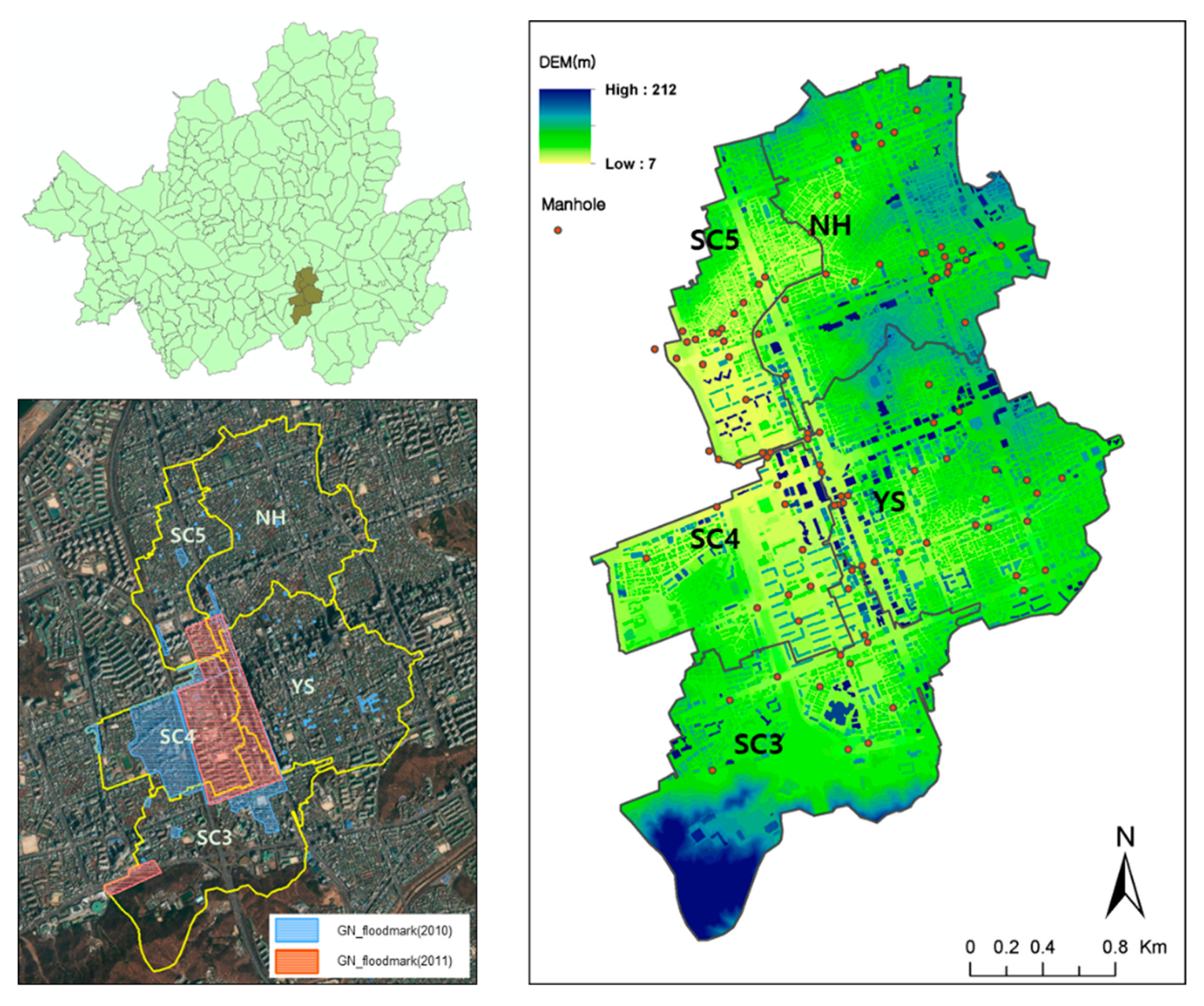
Seoul City manages its drainage system by dividing it into 239 districts to reflect the drainage system characteristics of each area. This study selected the following drainage sections around Gangnam Station as a study area: Nonhyun (NH), Yeoksam (YS), Seocho 3 (SC3), Seocho 4 (SC4), and Seocho 5 (SC5) (Figure 1). The total study area was 7.4 km2, and each drainage section area was 1.8 km2 (NH), 1.8 km2 (YS), 1.8 km2 (SC3), 1.1 km2 (SC4), and 0.8 km2 (SC5). The Seocho and Sapyung flood pumping stations are located in the study area, and rainwater from both are pumped to the Banpo river. Pump operation in the study area around Gangnam Station was included in the SWMM.
The study area around Gangnam Station is relatively low-land compared to adjacent areas and has a complex sewer pipe system, which is vulnerable to inundation due to heavy rains. The study area experienced record inundation areas of 1.4 km2 and 1.1 km2 due to torrential rains on 21 September 2010 and 27 July 2011, respectively.
2.2. Rainfall Data
The rainfall data used as input to the inundation prediction model were actual rainfall and scenario rainfall data. A time distribution method was applied in Seoul city to generate the scenario rainfall data. Generally, the most widely used method requires statistically analyzing the temporal distribution describing total rainfall and then determine the most suitable temporal distribution. This study applied Huff’s quartile method using all time distribution data from Huff’s first-quartile, second-quartile, third-quartile, and fourth-quartile. This technique is mainly used as a time distribution method for designing rivers and drainage systems in Korea [25]. The reason for using Huff’s method is that the peak value of rainfall is higher than other temporal distribution methods (e.g., Mononobe, Yen-Chow, Alternating block) in this study area, and it is judged to be adequate data for extreme urban flooding prediction. The 24 sets of scenario rainfall data correspond to durations of 1 h in 10 mm increments of rainfall, ranging from 50 mm to 100 mm in total. In addition, for rainfall over a period of 2 or 3 h, a total of 80 rainfall events were used with Huff’s temporal distribution data on rainfall frequency of 2, 3, 5, 10, 20, 30, 50, 70, 80, and 100 years periods. As a result, this study used 104 sets of scenario rainfall data as the input data to the prediction model and for rainfall conditions in the 1D urban runoff analysis program. Furthermore, the rainfall data became the input rainfall conditions to create the maximum inundation map that configured the input vector in SOFM. Detailed regional observation data from the Automatic Weather System (AWS) managed by the Korea Meteorological Agency (KMA) were used for actual torrential rainfall data alongside scenario rainfall data. AWS rainfall data over a 6 h period were used based on peak rainfall to retain the characteristics of realistic heavy rainfalls, considering that the duration of the 1 to 3 h scenario rainfall was not long. The following 20 torrential rainfall events reported by the AWS for Korea Meteorological Agency, which resulted in serious damages recently, were also used as the actual input torrential rainfall data in the SWMM and prediction model: Gangnam in 21 September 2010, 27 July 2011, 15 August 2012, and 22 July 2013; Seocho in 21 September 2010, 27 July 2011, 15 August 2012, and 22 July 2013; Busan in 16 July 2009, 27 July 2011, 15 July 2012, 25 August 2014, and 11 September 2017; Cheongju in 16 July 2017; Ulsan in 5 October 2016 and 11 September 2017; Changwon in 25 August 2014 and 5 October 2016; Incheon in 23 July 2017; and Cheonan in 16 July 2017. Accordingly, this study aimed to consider all scenario rainfall data with 1, 2, 3, and 6 h durations to account for various rainfall amounts and distributions.
3. Methodology
3.1. Construction of Database
To implement flood prediction, a flood database should be developed in advance by considering various probable rainfall scenario data. To do this, reliable hydraulic analysis programs should be used, and the inundation characteristics of the study area must be identified accurately in advance through various flood simulations.
In this study, 104 scenarios and 20 actual torrential rainfalls were used for 1D/2D simulations. The overflow from each manhole due to lack of flow conveyance could be calculated through using the SWMM results. In addition, a square grid (5 m × 5 m) was constructed with LiDAR data to reflect the shapes of buildings and roads, and 2D hydraulic analysis of a finite differential method was conducted using the 1D analysis results as the boundary condition. The rainfall, overflow, and inundation map data were saved as a database for training SVNARX and SOFM. Figure 2 shows the process for building the database.
3.2. Gamma Test
Although a large number of studies on preprocessing analysis were conducted, the problem of lag time and selection of optimal input data has not been solved. GT is a nonlinear modeling analysis technique that helps quantify the extent to which numerical input–output data can be expressed as a smooth, reliable model [26]. The basic concept is differentiated from existing nonlinear analyses in that it employs x vector values as input data and targets differentiable linear (or smooth) data models that can influence the output. Here, the assumed smooth model can be expressed as follows:
where the input vectors are vectors confined to some closed bounded set . Without loss of generality, the corresponding outputs are scalars; it can be assumed that the mean of the distribution of r is zero [27]. Here, the input data x and output data y should be continuous real variables with imposed boundary conditions. GT calculates the mean-squared -th nearest neighbor distances and the matching . Although the GT is an unknown function, it can be used to directly estimate Var(r) from data as follows:
and is:
Finally, the fitted regression line passes through and as follows:
To estimate the invariant noise, can be used and is expressed as follows:
The above nonlinear analysis technique was used to estimate the optimum parameters in SVNARX with regard to the time delay. was used as the uncertainty index for the input combination. The tendency of and the results of SVNARX were compared based on the prediction lag time, and the effectiveness of the GT was examined.
3.3. Enhanced Recurrent Neural Network
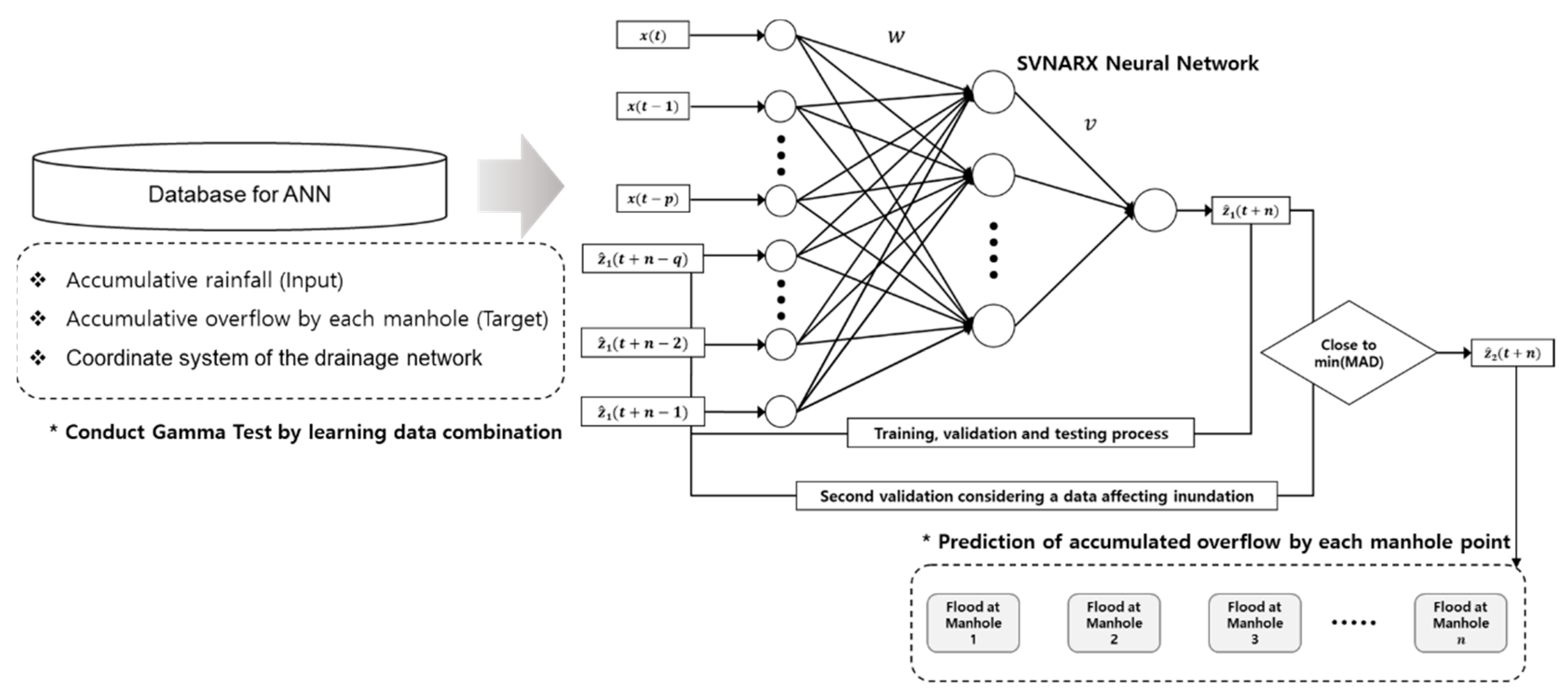
A variety of ANNs have been successfully applied to water resources, but they have not yet been effectively used to predict flooding prediction in urban areas. The reason is that real-time prediction results are difficult to obtain without regular observation data. To overcome the above drawbacks, NARX of an input layer, one hidden layer, and an output layer, and a feedback process was used in this study. NARX is a recurrent neural network that provides excellent time-series prediction [28,29]. The NARX used in many studies is excellent in itself, but in this study, SVNARX is proposed as an enhanced prediction method. SVNARX includes an additional verification process with actual rainfall-overflow data that incurred serious inundation damage in the study area. Error analysis during the second verification phase is performed using the median absolute deviation (MAD). This proposed neural network aimed to reduce the uncertainties and construct a prediction model that can flexibly cope with input data containing unknown target values, through double verification of heavy rainfall events over 6 h durations. The prediction process of accumulated overflow from manholes through the SVNARX is shown in Figure 3.
The accumulated overflow from manholes, which will be a target value and result of the learning process, are back-propagated to the input layer again to increase the number of input data. The above Figure 3 assumes that , , and . Here, refers to an input vector, and refers to an input vector for double verification. is the final output value, and is the output value at the secondary verification step. is the output vector in the hidden layer and the input value in the output layer. The input value and the one-step delayed output value are combined to produce vectors , and the -th element is . At time , the weighted sum (i.e., net neuron activity) with regard to the -th layer in the hidden layer can be calculated as follows:
The output value in the -th node in the hidden layer can be calculated as the weighted sum, which is input to the activation function .
The final value with regard to the -th node in the output layer and the resulting value with regard to the second verification can be represented as follows:
Assuming that the target value in the second verification phase at time is , the absolute mean error is given as follows:
SVNARX then performs forward propagation and back-propagation training using the above equations, and the weight value is updated in every cycle. The weight is updated to improve SVNARX by identifying the minimum allowable error during the second verification.
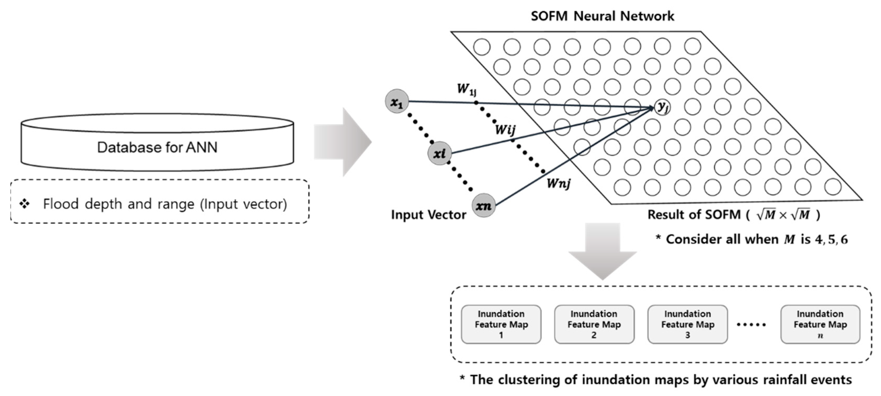
3.4. Clustering Method for Optimal Inundation Map
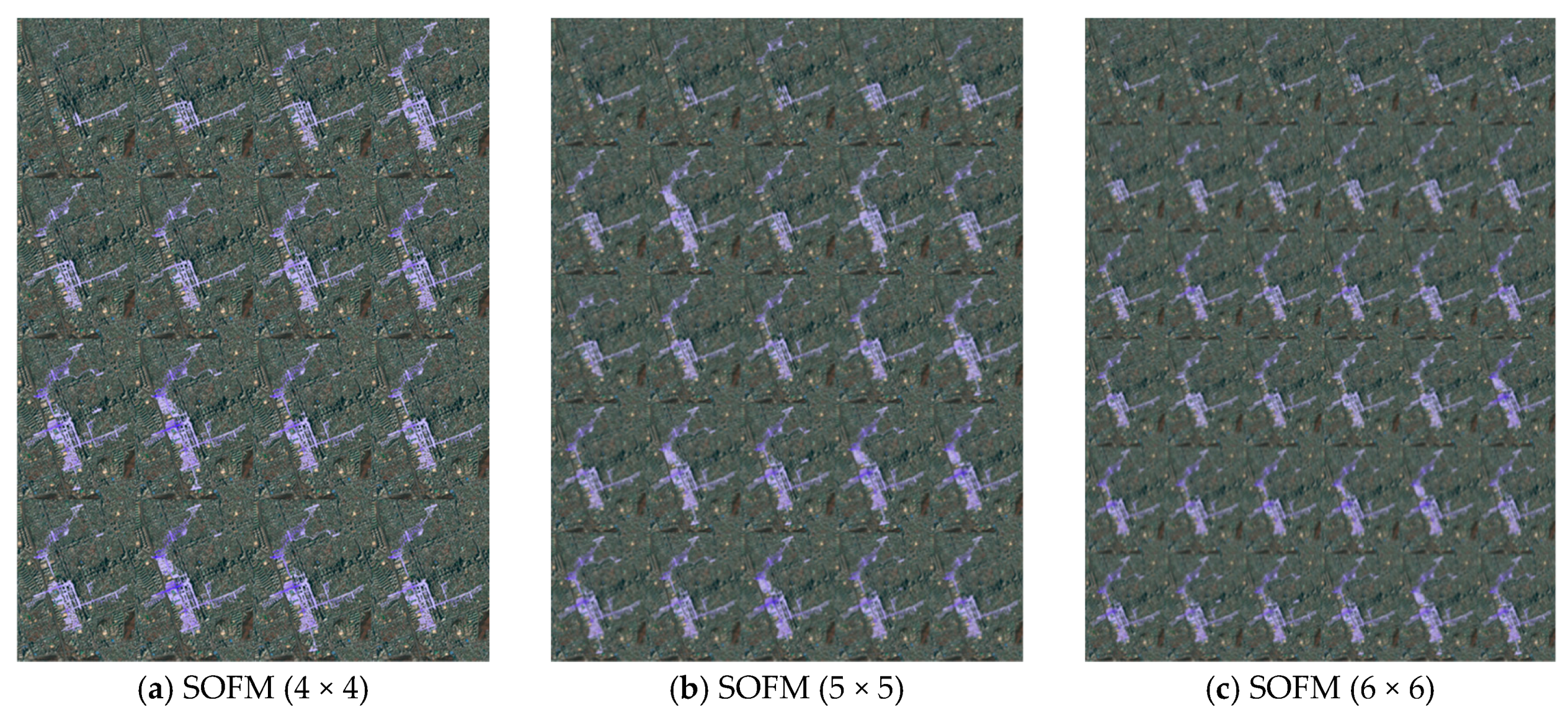
The SOFM was used to optimize the dimensions of the inundation map database. The SOFM, which is also called the Kohonen map, has become one of the most popular neural network methods for dealing with various problems in engineering and data analysis [30,31]. In addition, it can display representative data according to the inherent characteristics of the input data at specified dimensions (Figure 4). Optimal flooding maps which be prepared for prediction were generated in various dimensions (4 × 4, 5 × 5, 6 × 6) by using the characteristics of SOFM and the 2D inundation analysis results.
The SOFM training process based on inundation data is defined as follows. The distance between a given input value and weight value for all output neurons is calculated:
The shortest output neuron among all output neurons is searched and defined as a winner.
Only the winning neuron has an output value of 1, and the rest of the neurons have an output value of 0:
In summary, the output neuron that has the closest weight value with the given input data pattern becomes the winner, and only the winner has an output value of 1. This calculation is called winner-take-all. In the next step, the weight value of the winning neuron is modified to become closer to the current input pattern. Thus, the following weight value adjustment equation can be derived:
where refers to the current weight parameter of the -th output neuron and refers to the modified weight value parameter. The above equation plays a role in bringing the weight value closer to the input pattern by multiplying the difference between the input pattern and current weight value with a small constant value (learning rate ), and this is added to the current weight value.
3.5. Performance Comparison
The results from the prediction model were evaluated together with statistical analysis of the previously constructed input data. The performance was evaluated using the root mean square error (RMSE) to compare the commercial program results with prediction model results as a basic index, as defined in in Equation (16). The RMSE is an index that quantifies the error between the simulation value and prediction result.
RMSE-observations standard deviation ratio (RSR) was also considered for more statistical error analysis. RSR standardizes RMSE using the standard deviation in the observations, and it combines both an error index and some additional information. RSR was calculated as the ratio of the RMSE to the standard deviation of the measured data, as shown in Equation (17).
The coefficient of determination () was analyzed in addition to quantitative error analysis. The coefficient of determination is a square value of the correlation coefficient () and ranges from . This indicates that the simulated and predicted values have some constant tendencies, but the two values are not identical.
The Nash Sutcliffe efficiency coefficient (NSEC) was used to evaluate the prediction performance of the model presented in this paper. The NSEC is a standardized value of residual relative degree that ranges from . The closer the NSEC value is to 1, it indicates the more accurate the result of the prediction model. In Equation (18), refers to the simulated flow result, refers to the predicted flow result, and refers to the mean of the simulated flow result.
4. Application
4.1. 1D/2D Simulation and Verification
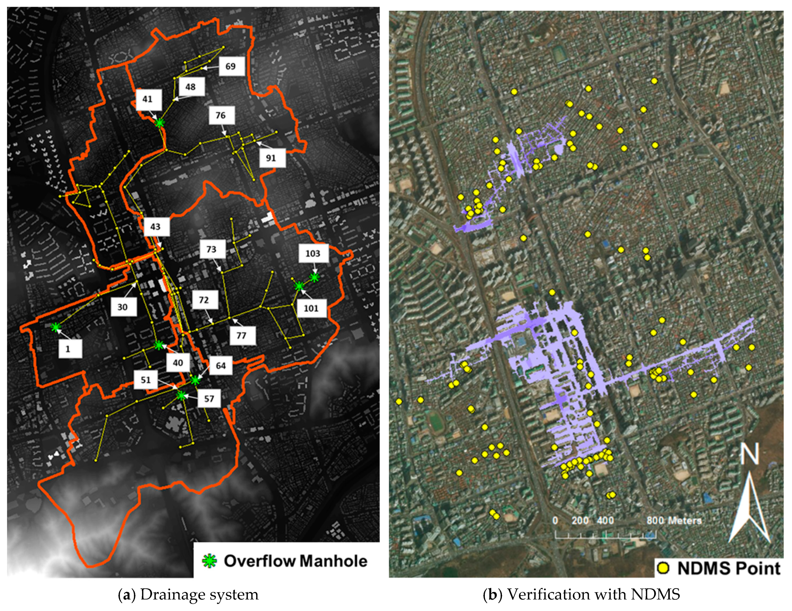
The optimum parameters suitable for 1D urban runoff analysis with SWMM were considered by referring to previous studies [32]. The overflow calculated with the 1D simulation was used as the input data of the 2D hydraulic analysis program based on the finite difference method. This method has advantages in that the technique is easy to understand, as a derivative of a governing equation is directly distinguished and the approximate difference equation is clearly revealed in the code. 2D inundation analysis was conducted within a 5 m × 5 m square grid with the digital elevation model (DEM), which was based on aerial LiDAR data. The number of manholes in the study area was estimated to be 103, and all manholes were used to train the prediction model. Figure 5 shows the drainage system which was used in this study and the main manholes in consideration with the number of overflows and frequency of flooding (Figure 5a).
Maximum flood depth maps were created for as many as the number of rainfall events, and they were processed to be used as the input in the SOFM. When creating maximum flood maps, the sufficient simulation time was needed to consider propagating the flood wave in between buildings and roads as much as possible. A composite roughness coefficient was used to analyze the surface flow while considering the optimum parameters suitable for inundation analysis in urban areas [33].
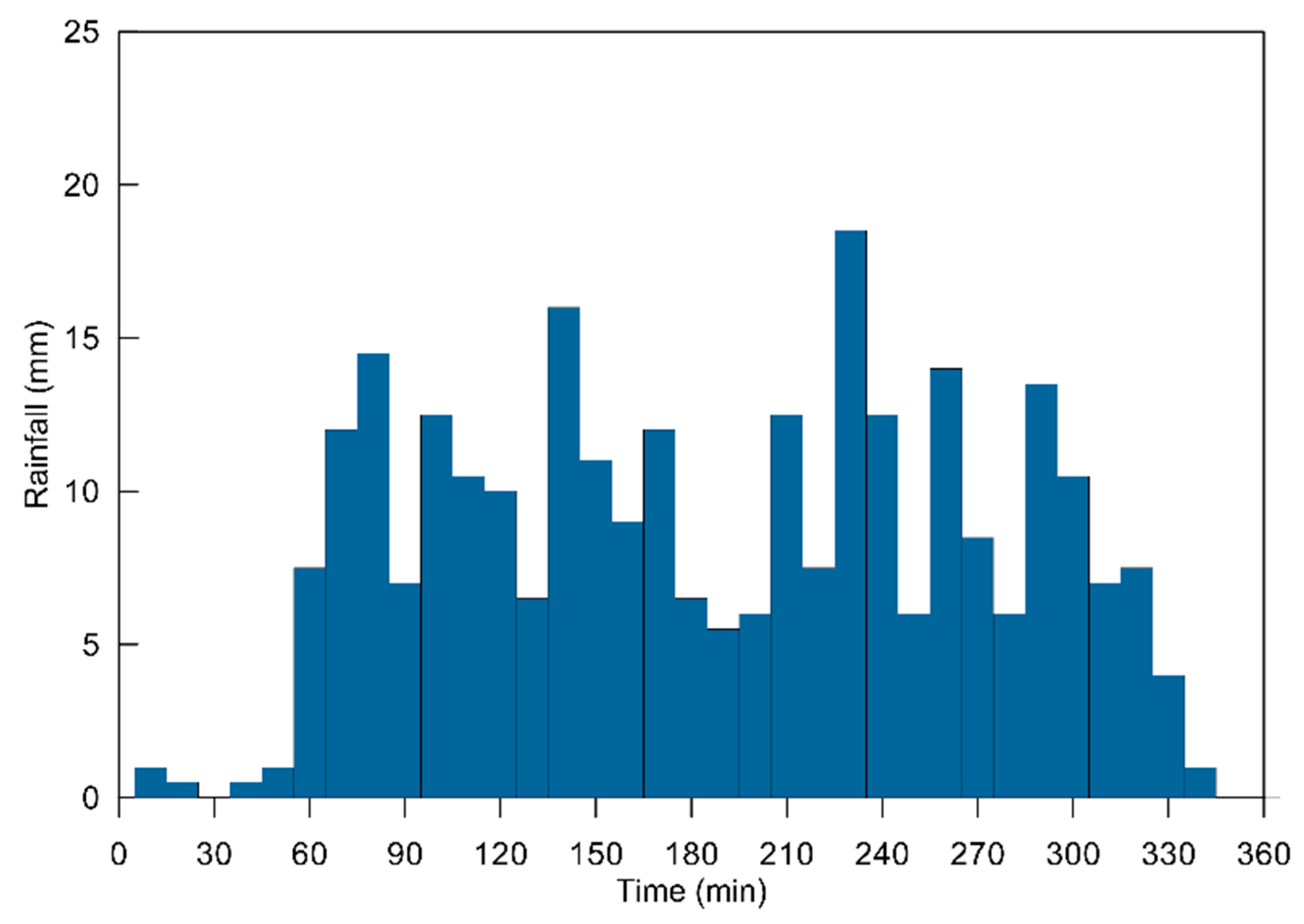
The National Disaster Management System (NDMS) about the rainfall data from 21 September 2010 were used to verify the hydraulic simulation. The NDMS data are GIS point data on the reported locations of nearby residents witnessing floods. In the simulation results, 6 manhole points overflowed, as shown in Figure 5a. The 2D simulation results for inundation analysis are shown in Figure 5b. The 6 h rainfall hydrograph is shown in Figure 6. Verification of the 2D model was intended to indicate the fitness of the inundation area about the NDMS data.
On 21 September 2010, NDMS reported data from 118 points, and 82 sites were included in the inundation analysis area. The goodness of fit was estimated to be 70%. The NDMS data is saved as the residents reporting point and is used to compensate damages, the NDMS data tends to contain excessive reporting points. Despite the characteristics of this NDMS data, the goodness of fit was obtained as 70%. The suitability evaluated in this study was estimated as reasonable results in terms of data for validation of the predictive model.
4.2. Input Data for SVNARX
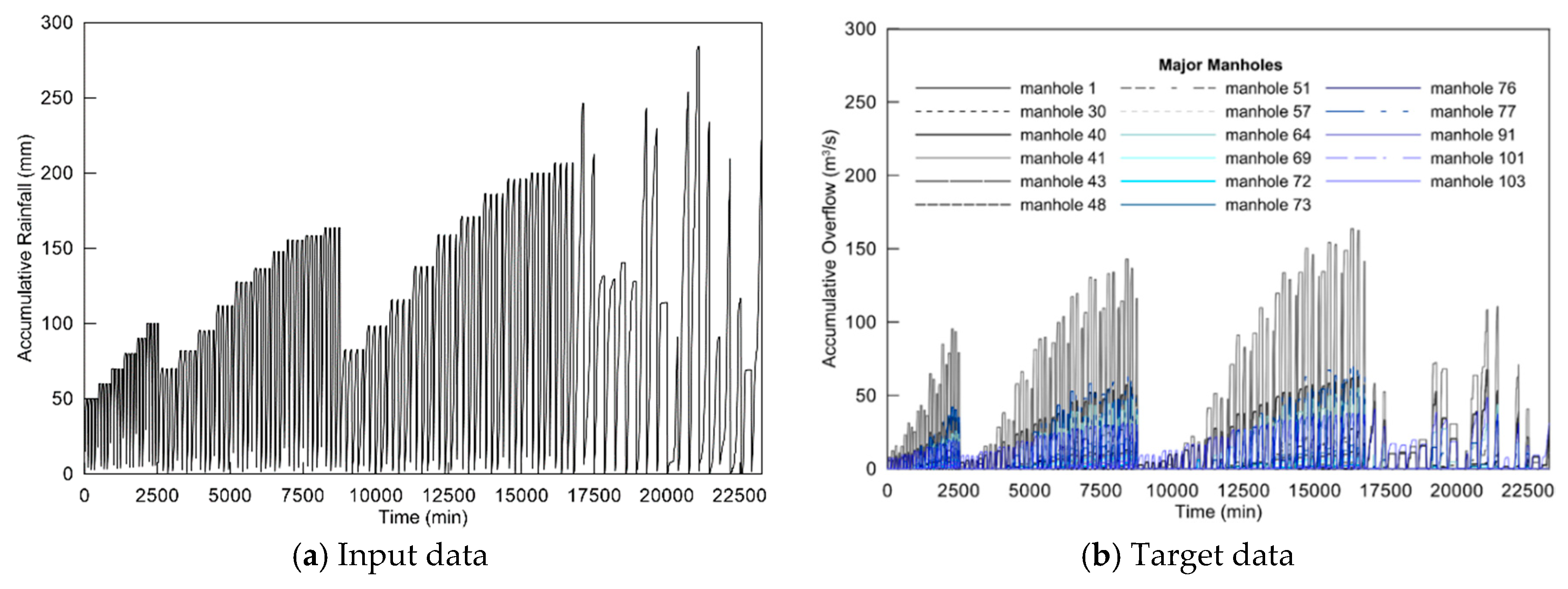
The aforementioned 124 rainfall events were used for input data for SWMM and SVNARX. These data were converted to an accumulated distribution and used to train SVNARX (Figure 7a). Overflows estimated from SWMM due to rainfall were also accumulated and used as the target values in SVNARX. To train the runoff relationships for various rainfall events, the accumulated distributions for each rainfall event and overflow at manholes were compiled as time-series data in ascending order. This preprocessing is intended to represent various rainfall runoff relationships and to predict accumulated overflows. Figure 7b shows a graph of the target accumulated overflow data at only 17 major manholes for clarity and brevity, although all manholes in the study area were considered.
Except the accumulated rainfall and overflow data presented in Figure 7, rainfall and overflow on 21 September 2010 estimated from SWMM were selected as the second set of data for validating SVNARX. The total rainfall in the second validation set was 278.5 mm over a duration of 6 h with 10 min intervals. In this study, the basic NARX and SVNARX were constructed to compare their predictive abilities, and the data presented in Figure 7 was used for training. A total of 122 rainfall events were used as common learning data, excluding the rainfall events for the second validation (21 September 2010 in Gangnam) and prediction (17 July 2011 in Gangnam). The second validation data set for 21 September 2010 was only used in SVNARX. The applicability of SVNARX was subsequently considered.
4.3. Prior Investigation of Uncertainties
The uncertainty in the input dataset was investigated using GT. 10 values near neighbors were used, and the uncertainty investigation was conducted based on lag time and the time delay parameters in SVNARX and NARX. The input data for modeling a neural network were used here, except the data used in secondary validation. The results are presented in Table 1; these results are divided into three cases with different lag times. The values of gamma (), gradient (), standard error, , and the number of nearest neighbors from the GT results are presented.
The uncertainty investigation results improved as the time delay parameter increased, from Case 1 to Case 3 (i.e., as the number of feedback target vectors increased). In particular, a significant change in can be seen, and the value that estimates scale invariant noise also improved significantly. According to Table 1, the input data for Case 3 is most suitable for use in SVNARX and NARX. The uncertainty analysis presented in this study was intended to compare the tendency in the predicted results for various time parameters with the GT results to examine the usefulness of prior uncertainty examination.
4.4. Prediction of Accumulated Overflows
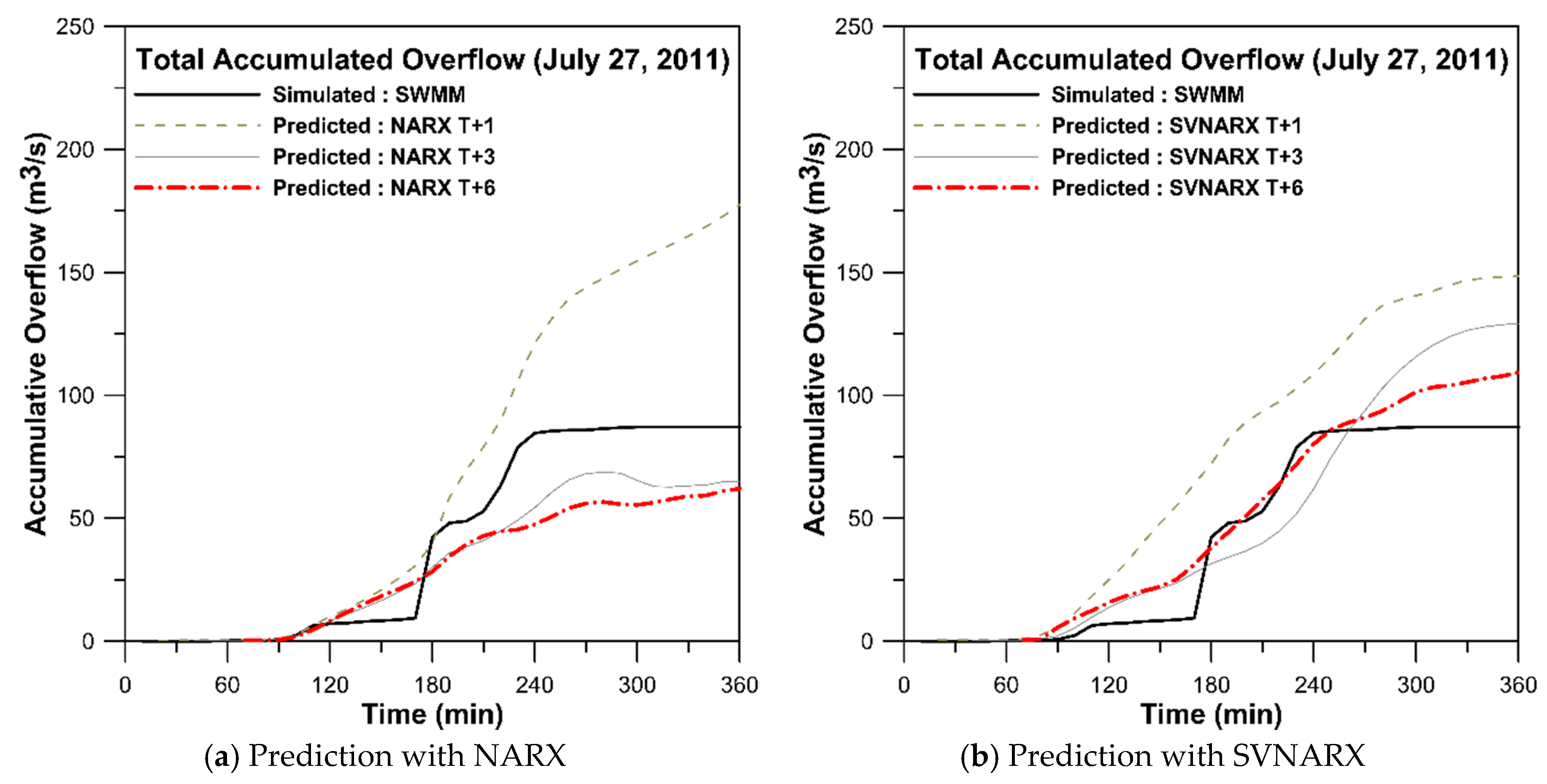
Real-time accumulated overflow from 103 manholes in the study area was predicted using SVNARX and NARX. The SVNARX model and the basic NARX model were compared using rainfall data from 27 July 2011 in Gangnam. The total rainfall was 183.5 mm over a duration of 6 h in 10 min intervals.
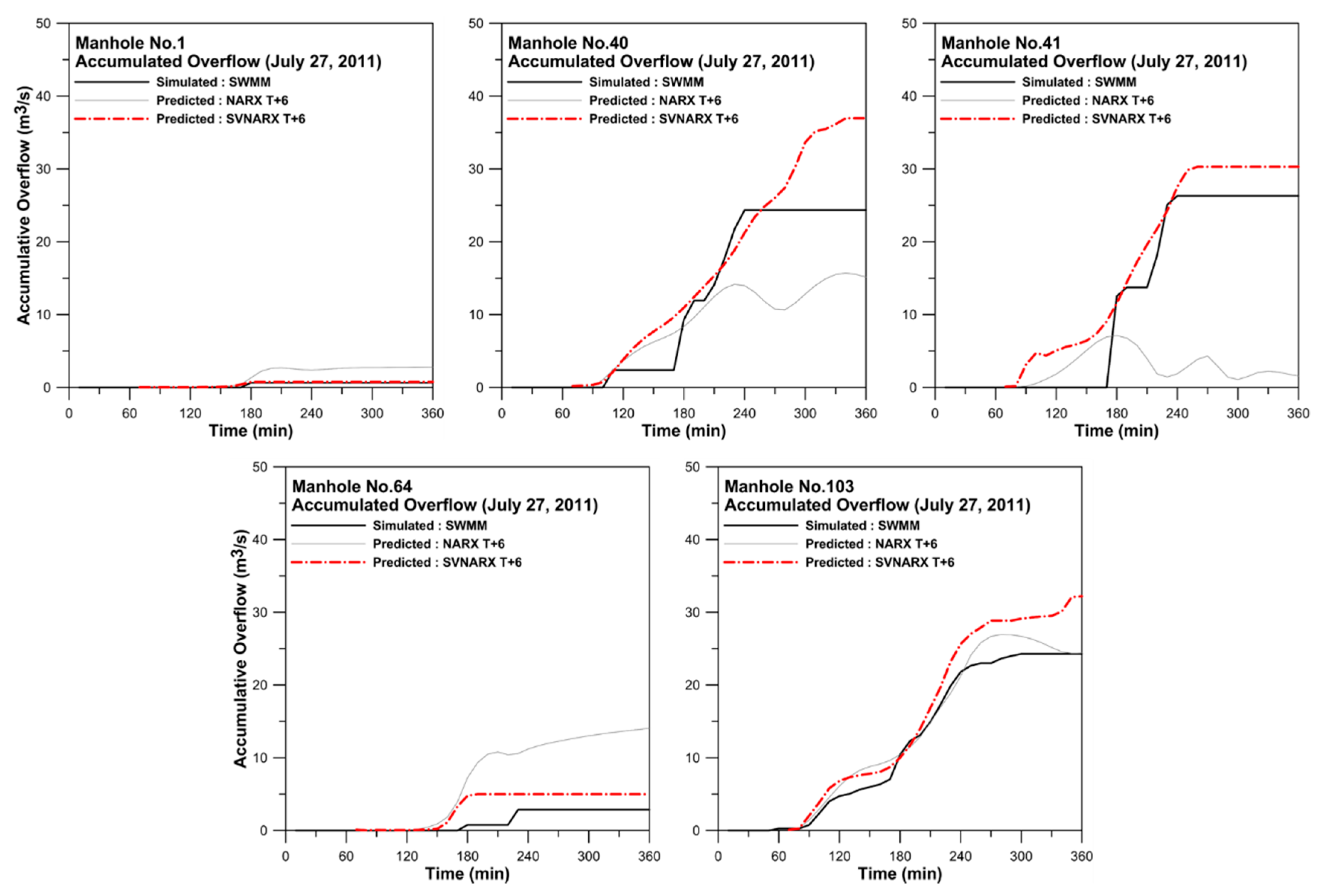
Error analysis was applied to the urban runoff analysis results in SWMM and the output data from the prediction model for various lag times. Table 2 shows the results of total overflow from all manholes. The values of RSR and were estimated as basic indices. In addition, the NSEC was used to evaluate the prediction performance of SVNARX and NARX. Table 3 shows the error analysis of the RMSE value at the manholes. Each error analysis was calculated by comparing with the simulation results. The SWMM and predicted accumulated overflow results reveal that manholes 1, 40, 41, 64, and 103 overflowed.
Table 3 shows that the error analysis results were better in SVNARX than NARX. In addition, some error values improved as the lag time increased for each model result. It is considered that this is because the number of target data with feedback to the input layer increased as the prediction lag time increased, making the training process more precise. The overall prediction results presented in Table 3 improved as the prediction lag time increased. As another feature, relatively inferior prediction results were revealed at manholes 40, 41, and 103, whose accumulated overflow was relatively large, whereas the other manholes with relatively small accumulated overflow exhibited superior results, as presented in Table 3. This result was obtained because the accumulated overflow in the final time term was able to follow the target value, whereas the accumulated overflow at the early and mid-time period was unable to follow the target value at manholes where accumulated overflow was large. In addition, as training was performed based on data with large accumulated overflow, larger accumulated overflow than the target value may be predicted at a given manhole. Figure 8 shows a comparison of the total accumulated overflow simulated with SWMM and that predicted with SVNARX and NARX.
The NARX model shows insufficient total overflow at a lag time of T + 3 and T + 6. On the contrary, the SVNARX model shows that performing a second validation produces sufficient overflow at all lag times, as indicated in Figure 8. The reason for this is that secondary verification was performed based on the rainfall-overflow data that caused severe flooding in the target area. In the Figure 9, prediction results at each manhole are presented when lag time of prediction is T + 6. Since this study aims to predict the inundation area, the SVNARX results indicating enough total overflow were considered more adequate and stable for predicting inundation.
4.5. Application of SOFM
2D flood analysis was conducted with regard to the scenario rainfall and actual torrential rainfall data from AWS in order to construct the input data for the SOFM. A total of 122 maximum flood depth maps (excluding the flood maps from 21 September 2010 and 17 July 2011 in Gangnam) were generated and configured with 258,279 square grids. Each map was used as an input neuron in the SOFM, and the results produced in the output neuron were also produced as a square grid map.
This study aimed to create clustering results that can reflect all maximum flood depth maps, based on sufficient iterative training, and convert the high-dimensional input data into low-dimensional data using the above characteristics. When the maximum flood depth map data were input, the number of output nodes was determined to be equal to the number of clustering dimensions designated by users, and training was performed in a winner-take-all manner. The batch weight value and bias adjustment self-training methods were used for training. In addition, the results were generated while maintaining their topographic position despite the multiple neural network learning iterations in order to reflect the spatial characteristics. The size of the input vector in the SOFM is . The SOFM results were divided into 4 × 4, 5 × 5, and 6 × 6 sizes. The optimum inundation map results from the SOFM are shown in Figure 10 for various output conditions. As shown in the Figure 10, the representable inundation maps can be more diverse as the dimension of the output data becomes higher. Prediction of inundation was performed by linking the results from SVNARX (NARX) and the SOFM while considering the total accumulated overflow. A simple adjustment using the multi-interpolation method enabled the linkage of SVNARX(NARX) and SOFM and the rapid prediction.
5. Inundation Map Prediction
Real-time inundation prediction was performed using SVNARX (NARX) and SOFM. In contrast to the previous prediction process, real-time prediction was performed here using only given rainfall data without target data, which are the results from SWMM when conducting prediction with SVNARX. In essence, it can provide real-time predictions of rainfall and runoff data that ensure a sufficient lead time since training is not required. In this study, SVNARX was compared to the basic NARX model by verifying the performance with rainfall data from 27 July 2011. The rainfall data for prediction was converted to accumulated distributions before being input to SVNARX and NARX.
The predicted total accumulated overflows for various lag times were linked to the SOFM results, while considering the output dimensions to predict the inundation map. The RMSE and NSEC values for the predicted results were compared as shown in Table 4. The RMSE (Root Mean Square Error) and NSEC (Nash Sutcliffe Efficiency Coefficient) values were calculated while considering inundation depth grids.
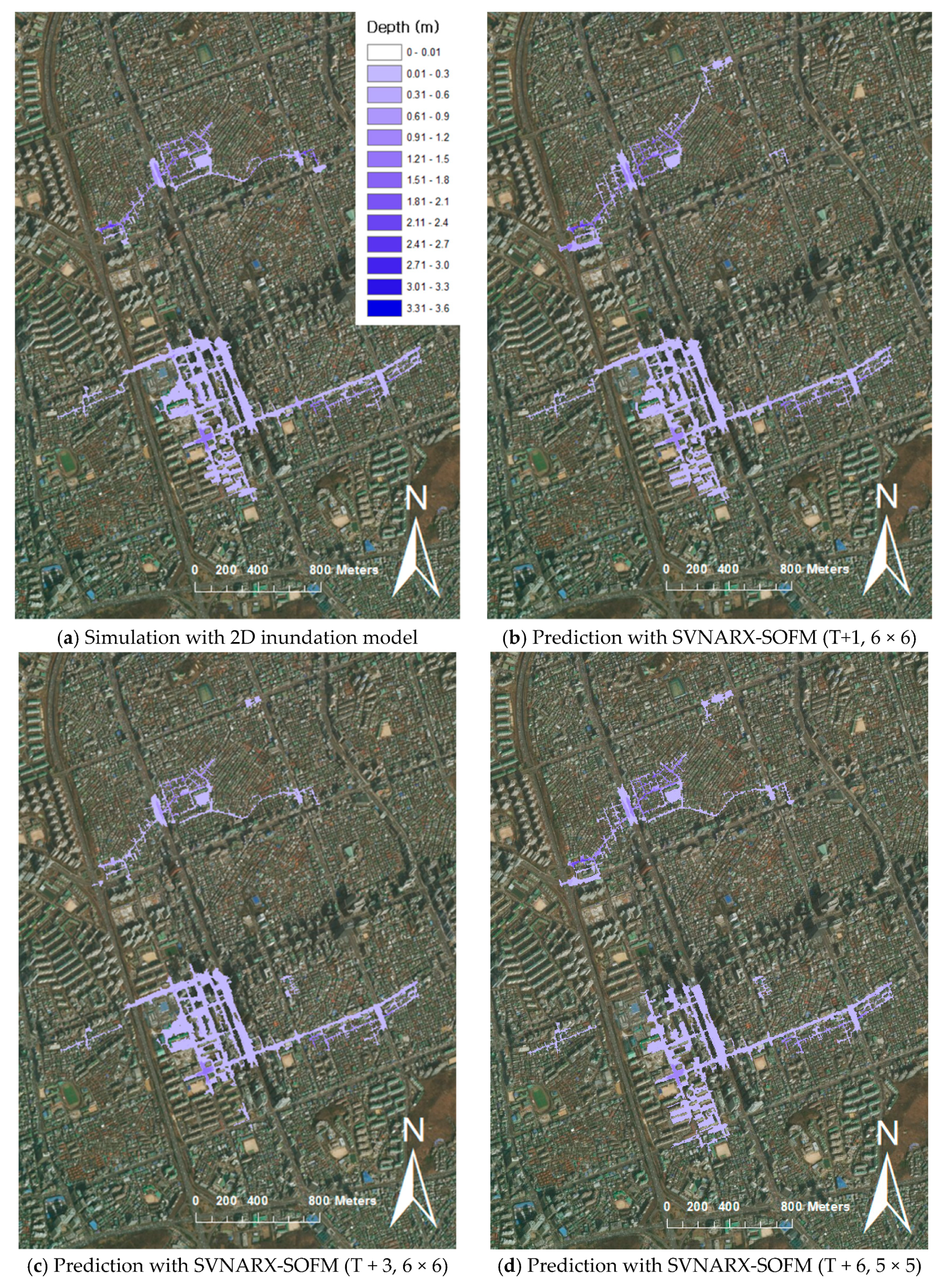
The simulated inundation results of torrential rainfall on 27 July 2011 show that the maximum flood amount was 151.71 m3/s and the maximum flood range was 6.46 km2. When the suitability of the inundation area was analyzed, the SVNARX model generally produced better results than NARX. In addition, the SVNARX (lag time of T + 3) results linked with SOFM 6 × 6 results were most suitable in the inundation area. The value of RMSE decreased when the inundation map was predicted with the SVNARX results. The NSEC value improved when using the SVNARX model, and the best NSEC value was produced with T + 6 lag time. This result arose based on adequate predicted total accumulated overflow results, as shown in Table 4. The suitability was also calculated by taking into account the number of predicted grids included in the simulated inundation map. In this study, the goodness of fit with the simulated inundation results was generally higher with SVNARX than with NARX. When the lag time was T + 1, the suitability improved to 66.77%, 76.79%, and 80.3% as the SOFM dimensions increased. The highest suitability was produced with a lag time T + 3 and the 6 × 6 SOFM as 80.4%.
Figure 11 shows the simulated inundation maps with the predicted results from the link between SVNARX and SOFM when conditions of 6 × 6 with T + 1, 6 × 6 with T + 3, and 5 × 5 with T + 6. The results of highest suitability according to the delay time conditions are showed in Figure 11, and the suitability of each result was 80.3% (Figure 11b), 80.4% (Figure 11c), and 70.79% (Figure 11d), in respectively. Because the primary objective of this study is to predict the overall flooding range rather than the depth of each grid, the results which showed good suitability with flood range were chosen for comparison with simulation results, despite the fact that the higher NSEC value was indicated in other conditions. In addition, RMSE and NSEC results in Table 4 were calculated from each grid’s depth value, which was not considered with volume and range of flood.
The prediction results show that the suitability of the inundation area was better in SVNARX than the basic NARX model, and the highest NSEC value was produced using the 6 × 6 SOFM clustering results. The hydraulic analysis simulation for a given size grid took 88 min, while the inundation prediction model proposed in this study took 1.3 min when performed with a standard desktop computer (Inter quad core i7-3770, 3.40 Ghz processor, 24.0 GB RAM). Based on these results, it is concluded that the predictive techniques presented in this study offer sufficient lead time.
6. Conclusions
This study aimed to develop an effective real-time inundation prediction technique using minimum data to ensure a sufficient lead time and prepare for urban flooding. SVNARX was constructed by applying rainfall and manhole overflow data, and scenario and actual torrential rainfall data were compared. A maximum inundation map data was created using 2D simulations with previous rainfall data, and the resulting inundation data were clustered to conduct real-time inundation prediction.
A second validation with SVNARX regarding actual torrential rainfall events that occurred on 21 September 2010 was performed in this study through a training procedure, and overflow at manholes and inundation under heavy rainfall on 27 July 2011 were predicted in real-time. The predicted accumulated overflow at manholes was used to predict the inundation map with SOFM. When comparing the basic NARX and SVNARX models, SVNARX produced better prediction results, except that the training time was longer than with NARX. A comparison of the results between the GT and the prediction results with SVNARX (NARX) indicates that the increasing or decreasing trends in error according to uncertainty were consistent to some extent. As the lag time for prediction increased to T + 1, T + 3, and T + 6, the GT and SVNARX results improved further, and the reliability of the predicted accumulated overflow at manholes also improved. However, the impact of GT was found to be more consistent with the trend of the predicted accumulated overflow at the manholes rather than the inundation map predicted with SOFM.
The inundated area predicted with SOFM shows that higher dimensions in SOFM produce better agreement with the 2D simulation results, compared with the use of lower dimensions in SOFM. Thus, the use of more than 6 × 6 dimensions in SOFM will be needed to improve the prediction of inundation on 27 July 2011. Because SOFM was not configured using an hourly flood map in this study, goodness of fit could be achieved even if the representation diversity in the optimal inundation map was insufficient. Since this is the inundation area fitness produced after calibration and validation with the 2D model, its reliability is high enough to be used in non-structural countermeasures against inundation in an urban area.
Finally, a verified prediction model was constructed with regard to actual torrential rainfall events. A system that can predict overflow and inundation maps was developed with this model. This result will contribute to establishing a measure to reduce flood damage through real-time prediction in the future. Furthermore, since this result was estimated using the link between the maximum inundation maps and total accumulated overflow in 10 min intervals, it can be used to predict flood depth maps that are separated by 10 min each. The results of this study will be applied to evacuation planning and sufficient response time for floods in urban areas.
Author Contributions
Conceptualization, K.Y.H.; Methodology, H.I.K.; Supervision, K.Y.H.; Writing original draft, H.I.K.; Writing—review & editing, H.J.K.
Funding
This research was funded by the Korea Ministry of Environment (MOE).
Acknowledgments
This subject is supported by the Korea Ministry of Environment (MOE) as the “Advanced Water Management Research Program” (18AWMP-B079625-05).
Conflicts of Interest
The authors declare no conflict of interest.
References
- Shin, S.Y.; Yeo, C.G.; Baek, C.H.; Kim, Y.J. Mapping Inundation Areas by Flash Flood and Developing Rainfall Standards for Evacuation in Urban settings. J. Korean Assoc. Geogr. Inf. Stud. 2005, 8, 71–80. [Google Scholar]
- Choi, S.M.; Yoon, S.S.; Choi, Y.J. Evaluation of high-resolution QPE data for urban runoff analysis. J. Korea Water Resour. Assoc. 2015, 48, 719–728. [Google Scholar] [CrossRef]
- Han, K.Y.; Lee, J.T.; Park, J.H. Flood inundation analysis resulting from levee-break. J. Hydraul. Res. 1998, 36, 747–760. [Google Scholar] [CrossRef]
- Tak, Y.H.; Kim, J.D.; Kim, Y.D.; Kang, B.S. A study on urban inundation prediction using urban runoff model and flood inundation model. Korean Soc. Civ. Eng. 2016, 36, 395–406. [Google Scholar] [CrossRef]
- Hsu, K.L.; Gupta, H.V.; Sorroshian, S. Artificial neural network modeling of rainfall-runoff process. Water Resour. Res. 1995, 31, 2517–2530. [Google Scholar] [CrossRef]
- Anmala, J.; Zhang, B.; Govindaraju, R.S. Comparison of ANNs and empirical approaches for predicting watershed runoff. J. Water Resour. Plan. Manag. 2000, 126, 156–166. [Google Scholar] [CrossRef]
- Garbrecht, J.D. Comparison of three alternative ANN designs for monthly rainfall-runoff simulation. J. Hydrol. Eng. 2006, 11, 502–505. [Google Scholar] [CrossRef]
- Toth, E.; Brath, A.; Montanari, A. Comparison of short-term rainfall prediction models for real-time flood forecasting. J. Hydrol. 2000, 239, 132–147. [Google Scholar] [CrossRef] [Green Version]
- Karamouz, M.; Razavi, S.; Araghinejad, S. Application of artificial neural networks in flood estimation. In Proceedings of the 4th International Conference on Decision Making in Urban and Civil Engineering, Porto, Portugal, 28–30 October 2004. [Google Scholar]
- Thirumalaiah, K.; Deo, M.C. Hydrological forecasting using neural netwokrs. J. Hydrol. Eng. 2000, 5, 180–189. [Google Scholar] [CrossRef]
- Trajkovic, S.; Todorovic, B.; Stankovic, M. Forecasting of reference evapotranspiration by artificial neural networks. J. Irrig. Drain. Eng. 2003, 129, 454–457. [Google Scholar] [CrossRef]
- Chang, L.C.; Shen, H.Y.; Wang, Y.F.; Huang, J.Y.; Lin, Y.T. Clustering-based hybrid inundation model for forecasting flood inundation depths. J. Hydrol. 2010, 385, 257–268. [Google Scholar] [CrossRef]
- Pan, T.Y.; Lai, J.S.; Chang, T.J.; Chang, H.K.; Chang, K.C.; Tan, Y.C. Hybrid neural networks in rainfall-inundation forecasting based on a synthetic potential inundation database. Nat. Hazard Earth Syst. Sci. 2011, 11, 771–787. [Google Scholar] [CrossRef] [Green Version]
- Chang, F.J.; Chen, P.A.; Lu, Y.R.; Huang, E.; Chang, K.Y. Real-time multi-step-ahead water level forecasting by recurrent neural networks for urban flood control. J. Hydrol. 2014, 517, 836–846. [Google Scholar] [CrossRef]
- Kalteh, A.M.; Hjorth, P.; Berndtsson, R. Review of the self-organizing map (SOM) approach in water resources: Analysis, modeling and application. Environ. Model. Softw. 2008, 23, 835–845. [Google Scholar] [CrossRef]
- Chang, L.C.; Shen, H.Y.; Chang, F.J. Regional flood inundation nowcast using hybrid SOM and dynamic neural networks. J. Hydrol. 2014, 519, 476–489. [Google Scholar] [CrossRef]
- Han, D.; Kwong, T.; Li, S. Uncertainties in real-time flood forecasting with neural networks. Hydrol. Process. 2007, 21, 223–228. [Google Scholar] [CrossRef]
- Hromadka, T.V.; Yen, C.C. A diffusion hydrodynamic model (DHM). Adv. Water Resour. 1986, 9, 118–170. [Google Scholar] [CrossRef]
- Marks, K.; Bates, P. Integration of high-resolution topographic data with floodplain flow models. Hydrol. Process. 2000, 14, 2109–2122. [Google Scholar] [CrossRef]
- Vojinovic, Z.; Seyoum, S.D.; Mwalwaka, J.M.; Price, R.K. Effects of Model Schematization, Geometry and Parameter Values on Urban Flood Modelling. Water Sci. Technol. 2011, 63, 462–467. [Google Scholar] [CrossRef]
- Fewtrell, T.J.; Duncan, A.; Sampson, C.C.; Neal, J.C.; Bates, P.D. Benchmarking Urban Flood Models of Varying Complexity and Scale Using High Resolution Terrestrial LiDAR Data. Phys. Chem. Earth A/B/C 2011, 36, 281–291. [Google Scholar] [CrossRef]
- Turner, A.B.; Colby, J.D.; Csontos, R.M.; Batten, M. Flood Modeling Using a Synthesis of Multi-Platform LiDAR Data. Water 2013, 5, 1533–1560. [Google Scholar] [CrossRef] [Green Version]
- Mason, D.C.; Giustarini, L.; Garcia-Pintado, J.; Cloke, H.L. Detection of flooded urban areas in high resolution Synthetic Aperture Radar images using double scattering. Int. J. Appl. Earth Observ. Geoinform. 2014, 28, 150–159. [Google Scholar] [CrossRef] [Green Version]
- Chen, J.; Hill, A.A.; Urbano, L.D. A GIS-based model for urban flood inundation. J. Hydrol. 2009, 373, 184–192. [Google Scholar] [CrossRef]
- Jang, S.H.; Yoon, J.Y.; Yoon, Y.N. A study on the improvement of Huff’s method in Korea: I. Review of applicability of Huff’s method in Korea. J. Korea Water Resour. Assoc. 2006, 39, 767–777. [Google Scholar]
- Remesan, R.; Mathew, J. Hydrological Data Driven Modelling: A Case Study Approach. In Earth Systems Data and Models; Springer: Berlin, Germany, 2015. [Google Scholar]
- Moghaddamnia, A.; Remesan, R.; Hassanpour Kashani, M.; Mohammadi, M.; Han, D. Comparison of LLR, MLP, Elman, NNARX and ANFIS Models with a case study in solar radiation estimation. J. Atmos. Sol. Terr. Phys. 2009, 71, 975–982. [Google Scholar] [CrossRef]
- Jiang, C.; Song, F. Sunspot forecasting by using chaotic time-series analysis and NARX network. J. Comput. 2011, 6, 1424–1429. [Google Scholar] [CrossRef]
- Shen, H.Y.; Chang, L.C. Online multistep-ahead inundation depth forecasts by recurrent NARX networks. Hydrol. Earth Syst. Sci. 2013, 17, 935–945. [Google Scholar] [CrossRef] [Green Version]
- Carlson, E. Self-organizing feature maps for appraisal of land value of shore Parcels. Artif. Neural Net. 1991, 2, 1309–1312. [Google Scholar]
- Back, B.; Sere, K.; Vanharanta, H. Data Mining Accounting Numbers Using Self-Organizing Maps; Finnish Artificial Intelligence Society: Vaasa, Finland, 1996. [Google Scholar]
- Ha, C.Y. Parameter Optimization Analysis in Urban Flood Simulation by Applying 1D-2D Coupled Hydraulic Model. Ph.D. Thesis, Kyungpook National University, Daegu, Korea, April 2018. [Google Scholar]
- Son, A.L.; Kim, B.H.; Han, K.Y. A study on prediction of inundation area considering road network in urban area. J. Korean Soc. Civ. Eng. 2015, 35, 307–318. [Google Scholar] [CrossRef]
Figure 1.
Study area and inundation trace.

Figure 2.
Flowchart for building a database for predictive modeling.

Figure 3.
Prediction process of SVNARX (The Second Verification Algorithm of Nonlinear Auto-Regressive with eXogenous inputs).
Figure 3.
Prediction process of SVNARX (The Second Verification Algorithm of Nonlinear Auto-Regressive with eXogenous inputs).

Figure 4.
SOFM (Self-Organizing Feature Map) for optimization of the 2D inundation map database.

Figure 5.
Drainage system (a) and 2D inundation model verification (b).

Figure 6.
Rainfall data from 21 September 2010 for verification.

Figure 7.
Training data for the prediction model.

Figure 8.
Total overflow prediction of NARX and SVNARX.

Figure 9.
Prediction results from each manhole in study area.

Figure 10.
Optimal flooding maps by SOFM dimension.

Figure 11.
Simulated and predicted inundation map.


Table 1.
Gamma test results for various prediction lag times.
| Parameter & Results | Case 1 | Case 2 | Case 3 |
|---|---|---|---|
| Parameter for model | p = 0, q = 1 | p = 0, q = 1:3 | p = 0, q = 1:6 |
| Prediction lag time | 10 min | 30 min | 60 min |
| Near neighbors | 10 | 10 | 10 |
| Gamma | 0.00624345 | 0.00189670 | 0.0016401 |
| Gradient | 0.67884798 | 0.18325886 | 0.10749 |
| Standard error | 0.00061490 | 0.00032968 | 0.00033552 |
| V-ratio | 0.02497381 | 0.00758682 | 0.0065606 |
Table 2.
Error analysis of the predicted total accumulative overflow.
| Model | Lead Time | RSR | R-Square | NSEC |
|---|---|---|---|---|
| NARX | T + 1 | 2.8293 | 0.9098 | 0.4532 |
| T + 3 | 1.1808 | 0.9578 | 0.3029 | |
| T + 6 | 1.7967 | 0.9438 | 0.7418 | |
| SVNARX | T + 1 | 0.5737 | 0.9396 | 0.5973 |
| T + 3 | 0.7368 | 0.9483 | 0.9092 | |
| T + 6 | 0.8413 | 0.9531 | 0.9353 |
Table 3.
RMSE (Root Mean Square Error) value at each manhole.
| Model | Lead Time | RMSE (m3/s) | ||||
|---|---|---|---|---|---|---|
| Manhole No.1 | Manhole No.40 | Manhole No.41 | Manhole No.64 | Manhole No.103 | ||
| NARX | T + 1 | 6.0345 | 10.7689 | 9.1399 | 23.7141 | 4.1777 |
| T + 3 | 0.2061 | 5.9846 | 14.2067 | 6.1731 | 1.5472 | |
| T + 6 | 1.5513 | 7.6038 | 17.043 | 7.7354 | 1.7977 | |
| SVNARX | T + 1 | 0.4359 | 15.8942 | 15.6102 | 1.1582 | 11.9519 |
| T + 3 | 0.2041 | 12.4705 | 8.35748 | 2.0794 | 3.2184 | |
| T + 6 | 0.1142 | 6.2444 | 4.3667 | 2.3247 | 5.3098 | |
Table 4.
Inundation predictions for various SOFM dimensions.
| Error | Model | SOFM 4 × 4 | SOFM 5 × 5 | SOFM 6 × 6 | ||||||
|---|---|---|---|---|---|---|---|---|---|---|
| T + 1 | T + 3 | T + 6 | T + 1 | T + 3 | T + 6 | T + 1 | T + 3 | T + 6 | ||
| RMSE (m) | NARX | 0.052 | 0.055 | 0.055 | 0.054 | 0.057 | 0.057 | 0.051 | 0.057 | 0.057 |
| SVNARX | 0.048 | 0.045 | 0.045 | 0.044 | 0.041 | 0.041 | 0.049 | 0.041 | 0.034 | |
| NSEC | NARX | 0.721 | 0.684 | 0.691 | 0.703 | 0.661 | 0.667 | 0.733 | 0.66 | 0.667 |
| SVNARX | 0.763 | 0.788 | 0.791 | 0.799 | 0.823 | 0.825 | 0.753 | 0.825 | 0.883 | |
© 2019 by the authors. Licensee MDPI, Basel, Switzerland. This article is an open access article distributed under the terms and conditions of the Creative Commons Attribution (CC BY) license (http://creativecommons.org/licenses/by/4.0/).
Share and Cite
MDPI and ACS Style
Kim, H.I.; Keum, H.J.; Han, K.Y. Real-Time Urban Inundation Prediction Combining Hydraulic and Probabilistic Methods. Water 2019, 11, 293. https://doi.org/10.3390/w11020293
AMA Style
Kim HI, Keum HJ, Han KY. Real-Time Urban Inundation Prediction Combining Hydraulic and Probabilistic Methods. Water. 2019; 11(2):293. https://doi.org/10.3390/w11020293
Chicago/Turabian StyleKim, Hyun Il, Ho Jun Keum, and Kun Yeun Han. 2019. "Real-Time Urban Inundation Prediction Combining Hydraulic and Probabilistic Methods" Water 11, no. 2: 293. https://doi.org/10.3390/w11020293
Note that from the first issue of 2016, this journal uses article numbers instead of page numbers. See further details here.