Differentiation in Aquatic Metabolism between Littoral Habitats with Floating-Leaved and Submerged Macrophyte Growth Forms in a Shallow Eutrophic Lake


Hellenic Centre for Marine Research (HCMR), Institute of Marine Biological Resources and Inland Waters, 46.7 km of Athens—Sounio Ave., 19013 Anavyssos, Attiki, Greece
*
Author to whom correspondence should be addressed.
Water 2019, 11(2), 287; https://doi.org/10.3390/w11020287
Submission received: 16 January 2019
/
Revised: 1 February 2019
/
Accepted: 2 February 2019
/
Published: 6 February 2019
(This article belongs to the Section Water Quality and Contamination)
Abstract
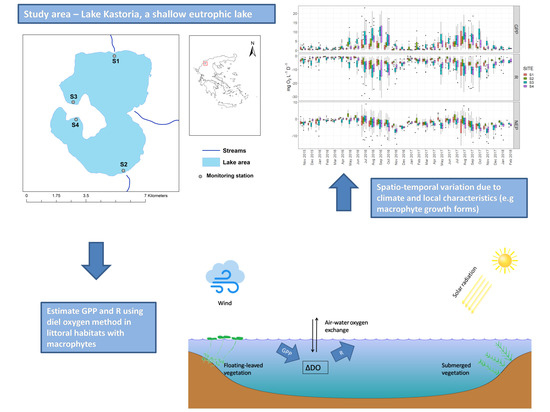
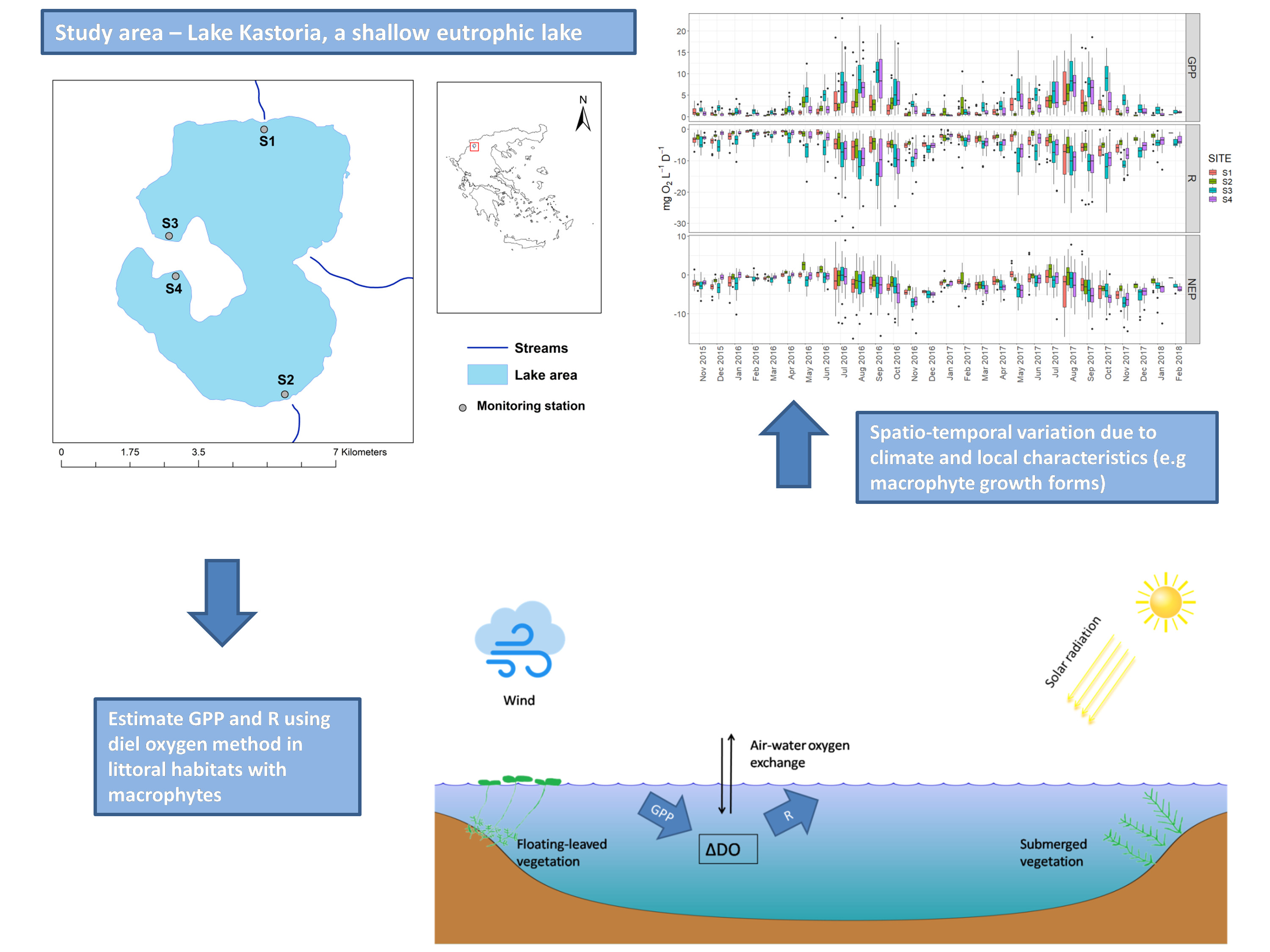
:The metabolic balance between gross primary production (GPP) and ecosystem respiration (R) is known to display large spatial and temporal variations within shallow lakes. Thus, although estimation of aquatic metabolism using free-water measurements of dissolved oxygen concentration has become increasingly common, the explanation of the variance in the metabolic regime remains an extremely difficult task. In this study, rates of GPP, respiration (R) and the metabolic balance (net ecosystem production, NEP) were estimated in four littoral habitats with different macrophyte growth forms (floating-leaved vs submerged) over a 28-month period in lake of Kastoria (Greece), a shallow eutrophic lake. Our results showed that net heterotrophy prevailed over the studied period, suggesting that allochthonous organics fuel respiration processes in the littoral. Temporal variation in the metabolic rates was driven mainly by the seasonal variation in irradiance and water temperature, with the peak of metabolic activity occurring in summer and early autumn. Most importantly, significant spatial variation among the four habitats was observed and associated with the different macrophyte growth forms that occurred in the sites. The results highlight the importance of habitat specific characteristics for the assessment of metabolic balance and underline the potentially high contribution of littoral habitats to the whole lake metabolism.
1. Introduction
Ecosystem metabolism is a fundamental process that integrates the rates of production and consumption of organic matter in a given ecosystem [1]. This practically means that the balance between productivity and consumption of organic compounds defines whether the ecosystem will act as source or sink for atmospheric carbon dioxide. Lakes in particular are considered as hot spots for global carbon cycles [2,3] because they can act as storage reservoirs and processors of terrestrial carbon [2]. Thus, it is not surprising that there is a growing interest for understanding the drivers of metabolism in lakes as it is of critical importance for describing responses of regional and global carbon fluxes to future environmental changes [3,4,5]. Yet, the dynamic nature of physicochemical and biological processes in lakes makes explanation of the variance in metabolic regime an extremely difficult task. Indeed, the variability in lake metabolism is related to numerous factors such as the availability of phosphorus and dissolved carbon in water [6,7,8], the lake morphometry [9,10,11], hydrodynamic processes and water temperature oscillations [6,12]. This implies that the role of lakes in the carbon cycling is not always obvious as it not only relies on the response of the ecosystem to dynamic processes, such as eutrophication, but also depends on the geographic context [13]. Consequently, gross primary production and ecosystem respiration may display large temporal and spatial variations within lakes resulting in shifts in metabolic state between autotrophy, that is when net ecosystem production is positive, and heterotrophy, when net ecosystem production is negative [14,15,16]
Estimation of aquatic metabolism using free-water measurements of dissolved oxygen concentration has become increasingly more common as the availability of new, cheap and reliable sensors facilitate high-frequency measurements and continuous monitoring of metabolic processes [4]. This technique is based on the assumption that changes in oxygen concentration reflect the biological balance between photosynthetic production and respiratory consumption as well as the physical exchange of oxygen between air and water. Thus, gross primary production (GPP), ecosystem respiration (R) and the metabolic balance (net ecosystem production, NEP) can be estimated throughout a 24-h period [9]. Once technical improvements in oxygen sensors made possible the continuous monitoring of oxygen concentration and relevant physico-chemical parameters, the diel oxygen technique has been widely used in limnology for assessing the temporal dynamics of aquatic metabolism and analyzing the main drivers [4].
Nevertheless, most studies on aquatic metabolism have been limited in north-temperate systems and concern the pelagic habitats without taking into consideration the metabolic processes that occur in the littoral [17]. Only a few studies have covered both pelagic and littoral habitats [18,19,20] and even fewer have taken into account the role of the littoral aquatic vegetation and periphytic communities [21]. In addition, there is a profound lack of studies that have dealt with the dynamics of ecosystem metabolism in shallow warm lakes. Particularly in polymictic shallow lakes, which are susceptible to warming and wind induced mixing effects, aquatic metabolism is expected to display highly dynamic behavior with abrupt changes within short periods (e.g., weeks) and to present larger variability in the littoral than the open water due to the presence of benthic littoral communities and their interaction with the land–water interface (e.g., benthic aquatic vegetation) [22].
The overall aim of this study was to expand our knowledge of spatiotemporal dynamics of metabolism in polymictic shallow lakes with emphasis placed on the role of aquatic vegetation that grows in littoral habitats. The specific objectives were to assess the spatiotemporal variations of metabolic balance in littoral habitats of a shallow polymictic lake and to identify the main drivers of metabolic estimates (GPP, R, NEP) regarding the aquatic vegetation. To this end we calculated metabolic estimates at four littoral habitats of a shallow polymictic Mediterranean lake for a 28-month period using an extensive dataset of continuous measurements of dissolved oxygen concentration and relevant physicochemical and climate parameters. Temporal and spatial dynamics were assessed with respect to special characteristics of the examined habitats (aquatic plants, surrounding land uses) and linear models were employed to identify the main drivers of GPP, R, and NEP. Our basic hypotheses were that the littoral habitats would be predominantly heterotrophic and that would display large variations in metabolism driven mainly by temperature and irradiance oscillations. We also expected that the spatial variation in metabolic rates would be determined primarily by the type of aquatic macrophyte growth from.
2. Materials and Methods
2.1. Site Description
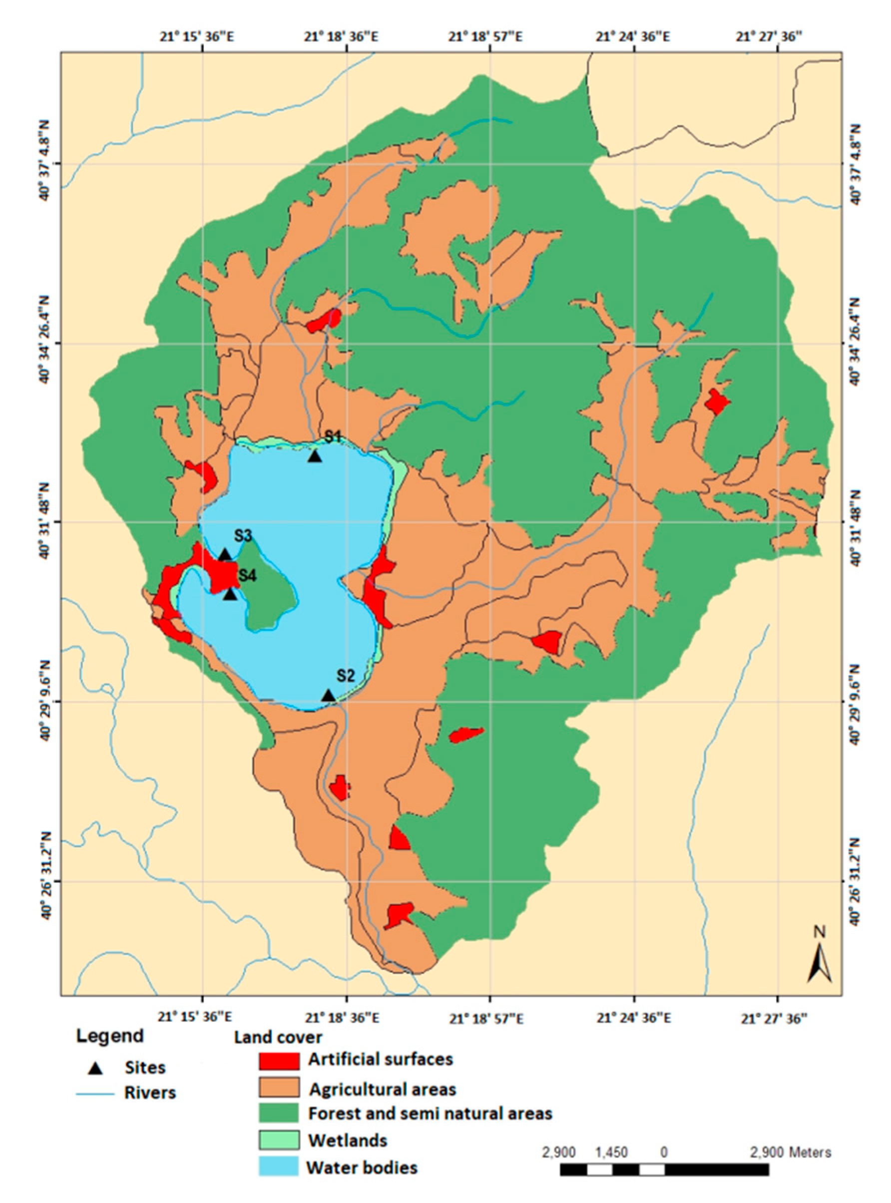
The study was conducted in Lake Kastoria situated in northern Greece (40°31′ N and 21°18′ E, Figure 1). The lake area covers approximately 28 km2, has a maximum depth of 9 m, an average depth of 4.4 m and a water retention time greater than 2 years (Table 1). Lake Kastoria is considered a highly eutrophic system with a history of toxic cyanobacterial blooms [23]. The land uses in the catchment are diverse with agricultures being dominant. The lake had been receiving sewage effluents from the city of Kastoria until 1995. Anthropogenic interventions in the lake include hydraulic adjustments, fish stock management, introduction of cyprinoids, and aquatic macrophyte cutting and removal. High concentrations of inorganic nitrogen and phosphorus have been reported from previous studies [23,24,25,26]. Elevated cyanobacteria biomass has also been reported in the past that is related with a history of toxic cyanobacterial blooms [27]. Aquatic vegetation of the lake is predominantly limited to the littoral zone since the high water turbidity constrains the growth of submerged hydrophytes in the deeper parts. The most common submerged macrophytes are Myriophyllum spicatum (L.) and Ceratophyllum demersum (L.). The floating-leaved Trapa natans (L.) forms extensive mats usually found at the eastern and western parts of the lake [24,25].
2.2. Collection of Data
The automated stations equipped with a sonde were deployed at the littoral zone of the lake at four sites with different habitat characteristics with respect to the local influences from the adjacent land uses, hydrological inputs and the dominant aquatic vegetation (Table 2). In addition, the four sites differ significantly in terms of impacts by human pressures and alterations in lake shore [28]. Site S1 is located at the northern part close to the mouth of a small stream. This part of the lake is influenced by the agricultural runoffs that originate from the cultivations in the adjacent area. The benthic vegetation is dominated by submerged macrophytes, mainly Myriophyllum spicatum and Ceratophyllum demersum. Site S2 is located at the south-eastern shore close to a small stream in which the lake outflows through a floodgate. The benthic vegetation in the site is characterized mainly by Myriophyllum spicatum and Ceratophyllum demersum. Sites S3 and S4 are located at the western part of the lake and are mostly influenced by the urbanized land uses of the city of Kastoria. The aquatic vegetation in these sites is characterized by the dominance of the floating-leaved macrophyte Trapa natans.
Measurements of dissolved oxygen concentration, water temperature and chlorophyll-a concentration were taken continuously at 1 m depth every 1 h for 28 months (Table 3). The sondes were equipped with a self-cleaning optical sensor for dissolved oxygen. The oxygen sensors were calibrated prior and after deployment every 30 days. No drifts of the sensor were observed between calibrations. Photosynthetically active radiation (PAR) and wind speed were obtained with a meteorological station placed at the eastern shore of the lake. All meteorological measurements were made at 10-min intervals and then averaged per hour for analysis. Wind speed was converted to wind speed at 10 m height based on the common exponential wind profile assumption [29]. This simple algorithm, which is based on a neutrally stable boundary layer assumption, is widely used for estimating standard wind speed at 10 m height from lower height measurements and requires less data than other more sophisticated methods that correct for atmospheric stability [30]. Gas exchange velocity (K600) was calculated using the Vachon and Prairie gas flux model [31]. Recently, it was shown by Dugan et al. [32] that the choice of gas flux model is of critical importance for metabolism studies as there is more uncertainty in model choice than in the parameterization of the metabolism model. Here we used the Vachon and Prairie model because it requires only the input of wind speed and lake area but provides similar estimations of K600 with those of surface renewal models that take into account other processes than wind that influence gas exchange [32]. All data were screened prior analysis to remove out-of-range values and anomalous measurements that were extreme outliers.
2.3. Estimation of Metabolic Balance
Metabolic estimates of GPP and community respiration (R) were calculated with a metabolism model that accounts for both process and observation error using a Kalman filter algorithm as described by Batt and Carpenter [33]. Besides the systematic error derived from the data generating process and the calculation process defined by the metabolism model (process error), error can also result from inaccuracies in the measurement of DO resulting in increasing variability (noisy data). A metabolism model using a Kalman filter makes the distinction between the two error types by incorporating two sets of equations that describe the process and observation components of the model [29]. This model excels in relation to simpler models since it provides more accurate estimates of metabolism components as shown by Batt and Carpenter [33]. The calculation of metabolism is achieved with linear regression models that fit the parameters ι and ρ using maximum likelihood. Parameter ι describes GPP per unit of incoming light and parameter ρ the average rate of respiration per natural log of water temperature. The equation that gives the modeled dissolved oxygen concentration is:
where at−1 is the modeled oxygen concentration of the previous state, ι and ρ are the parameters to be estimated, I is incoming light, logeT is the natural log of water temperature and F is the discrete atmospheric gas exchange and ε the process error. Observation error is estimated using observed values of DO. Then, GPP at a time step t can be estimated as:
And R as:
Model fitting, optimization, and calculation of daily estimates of GPP, R, and NEP (the metabolic balance expressed as GPP-R) were conducted in R with the function metab.kalman of the package LakeMetabolizer [29]. A detailed description of the equations is included in the publication of Winslow et al. [29]. Impossible estimations of GPP and R (negative GPP and positive R) were omitted from further analyses.
2.4. Statistical Analysis
Pearson correlations were run to explore potential relationships between daily metabolic rates and daily means of environmental variables. Then we employed linear models to investigate for the dependence of metabolic estimates on the wind speed at 10 m above surface, PAR, chlorophyll-a concentration (Chl-a), electrical conductivity (EC), water temperature and the sampling site as a factor predictor with four levels (S1,S2,S3, and S4). A second series of models was developed using monthly means to further examine the dependencies on metabolism at coarser time scale. For each metabolic estimate, a full model (all descriptors included) was built with the glm function in R [34]. Then using the dredge function from package MuMIN [35] we obtained the best possible model based on the ranking of the models according to the Akaike information criterion (AIC). Pseudo-R2 values for each model were computed with the r.squaredLR function. Prior to the statistical modeling, Box-Cox transformation was applied to all variables. In addition, Kruskal-Wallis was conducted to test for significant differences in environmental variables among the four sites.
3. Results
3.1. Spatiotemporal Dynamics of Environmental Parameters
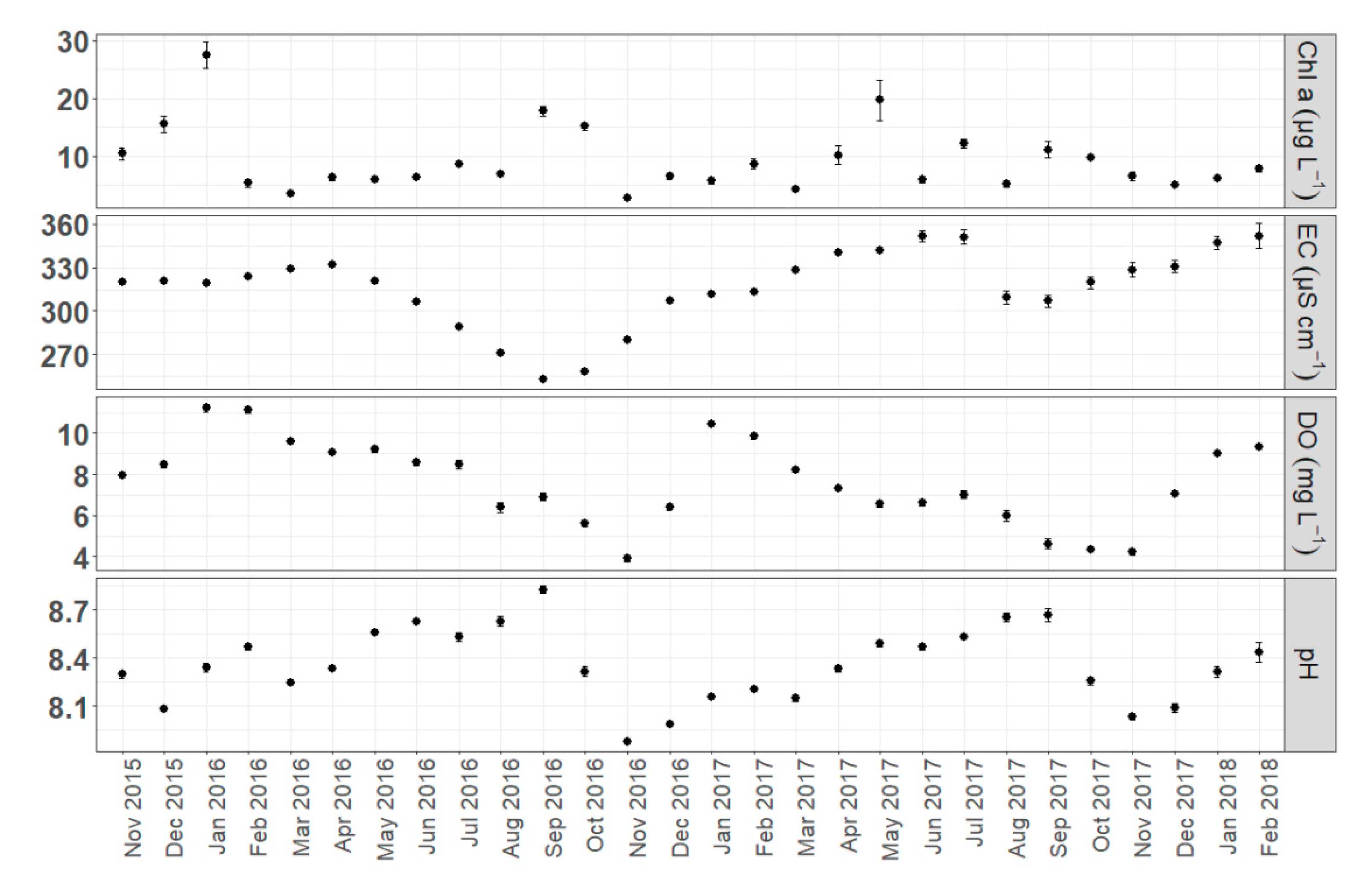
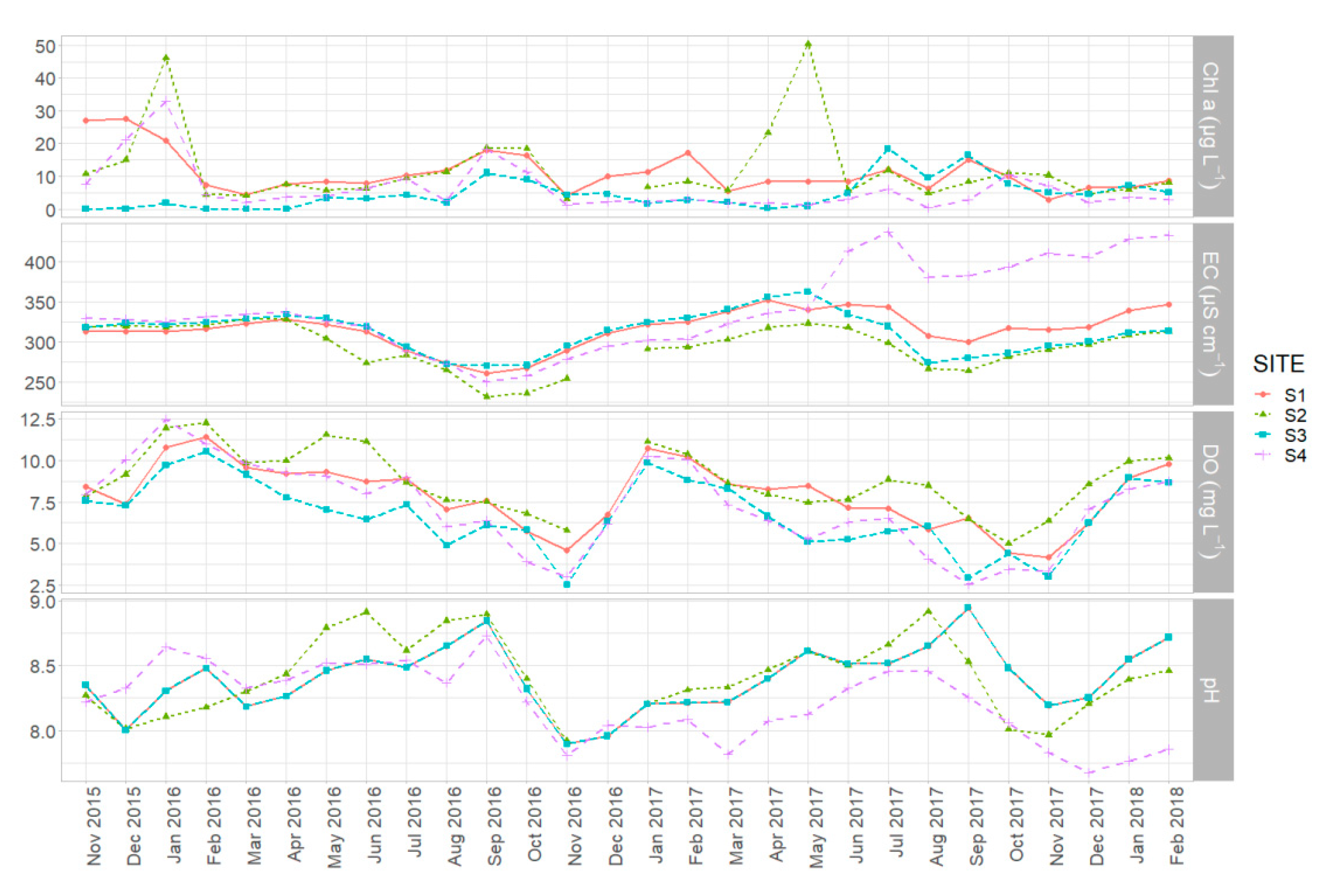
The results showed the expected seasonal trends in monthly means of the abiotic parameters calculated by pooled daily measurements (all sites included). The variation of dissolved oxygen concentration and pH followed a clear seasonal pattern in both years (Figure 2). Higher monthly means of DO were recorded in winter (January 2016, January 2017 and February 2018) followed by a declining trend until November (2016, 2017). The peak of mean monthly pH was observed in September, for both 2016 and 2017 (8.82 and 8.66 respectively), and the minimum in November (7.87 in 2016 and 8.03 in 2017). Conductivity also fluctuated seasonally showing an obvious decline until September followed by a recovery until early spring. Chl-a concentration showed a less obvious seasonal variation with peaks recorded in January, September, and October of 2016 and in May of 2017. By further examining the seasonal trends for each monitoring site we identify the same consistent pattern, but in parallel we can observe the presence of small spatial differences (Figure 3).
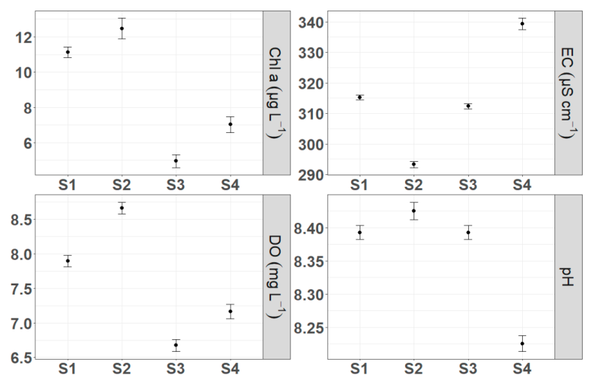
By comparing the investigated parameters among the four habitats we found statistically significant differences, highlighted by the Kruskal-Wallis test (Figure 4). S2 site presented the highest mean pH, DO concentration and Chl-a concentration and the lowest conductivity (8.42, 8.66 mg L−1, 12.46 μg L−1 and 293.29 μS cm−1 respectively). The highest conductivity and the lowest pH means were observed in site S4 (339.28 μS cm−1 and 8.22 respectively), while S3 was characterized by the lowest mean DO and Chl-a concentrations (6.67 mg L−1 and 4.94 μg L−1). Temporal trends were identical for all sites except for a significant increase of conductivity in site S4 that occurred from June 2017 until February 2018. In addition, site S2 exhibited a remarkable increase of Chl-a concentration in April and May of 2017 compared with the other sites.
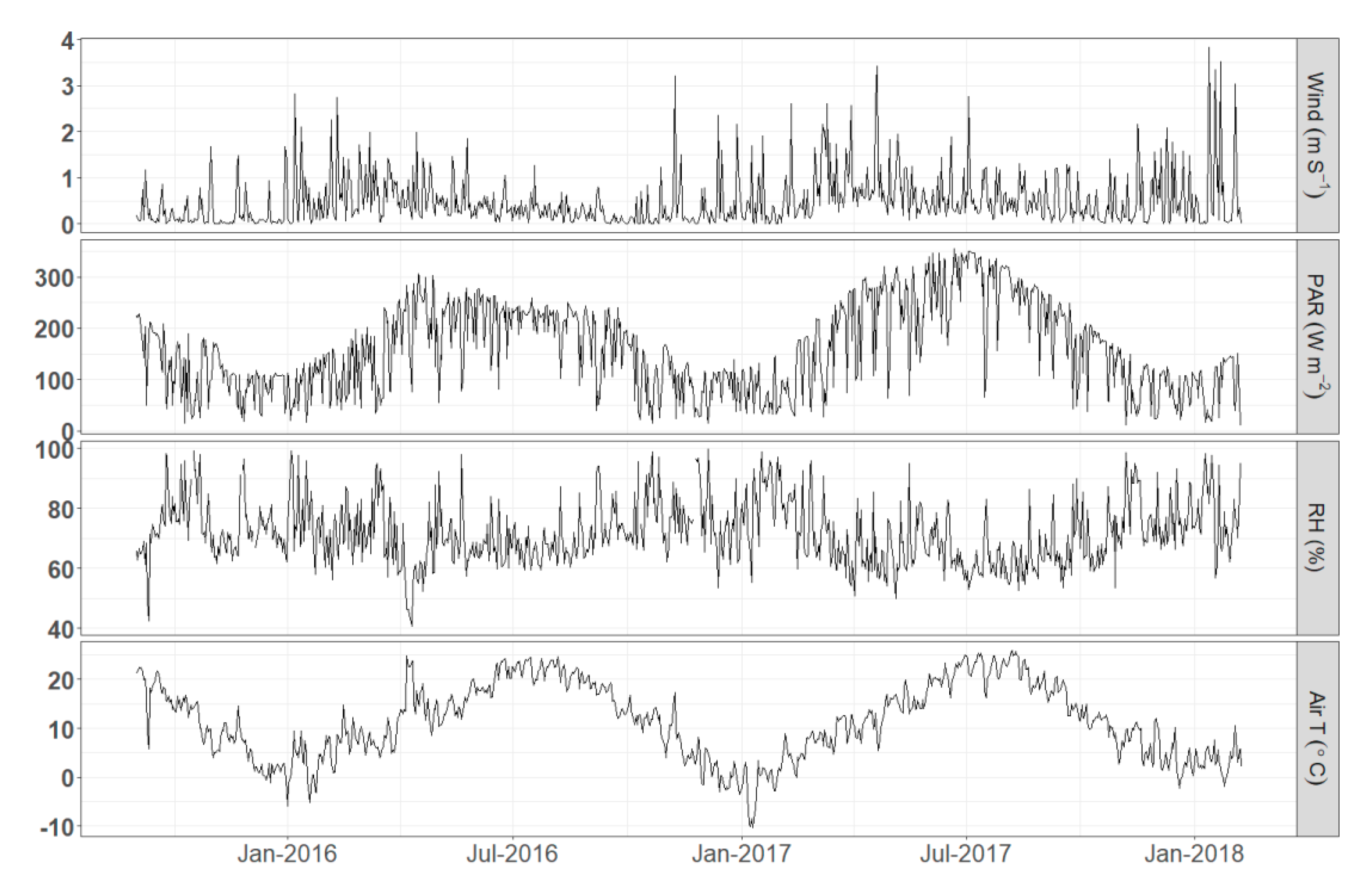
Concerning the meteorological parameters the variability showed the expected seasonality (Figure 5). It is worth noting the highly variable air temperature ranging from several degrees below 0 °C in winter up to 30 °C during the summer. Wind speed in general remained low with events of higher value (but no more than 4 m/s) occurring more frequently during winter.
3.2. Temporal Dynamics of Metabolic Estimates
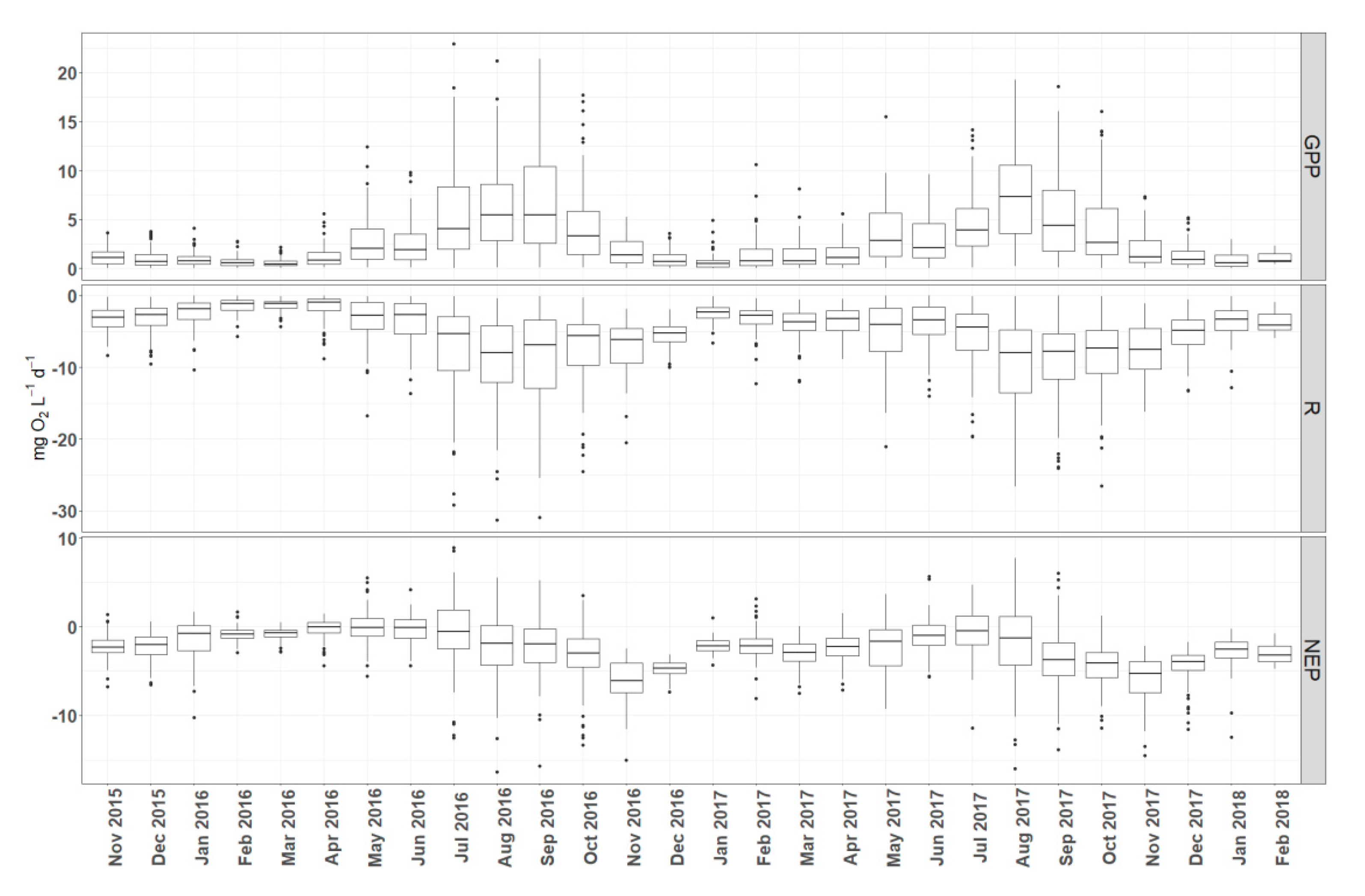
Rates of GPP and R (calculated from pooled daily estimates from the four sites) increased during spring, reached a maximum in late summer (August and September) and declined in fall and winter for both years (Figure 6). High rates of respiration persisted until November (2016 and 2017) and showed a sharp decrease in early winter. Annual rates of GPP were 2.84 mg L−1d−1 O2 in 2016 and 3.19 mg L−1 d−1 O2 in 2017. Annual rates of R were 4.86 mg L−1 d−1 O2 in 2016 and 5.60 mg L−1 d−1 O2 in 2017. The sites were net heterotrophic with annual average 1.93 NEP of mg L−1 d−1 O2 in 2016 and 2.84 mg L−1 d−1 O2 in 2017. The highest NEP mean monthly values occurred during autumn and specifically in November of 2016 and 2017.
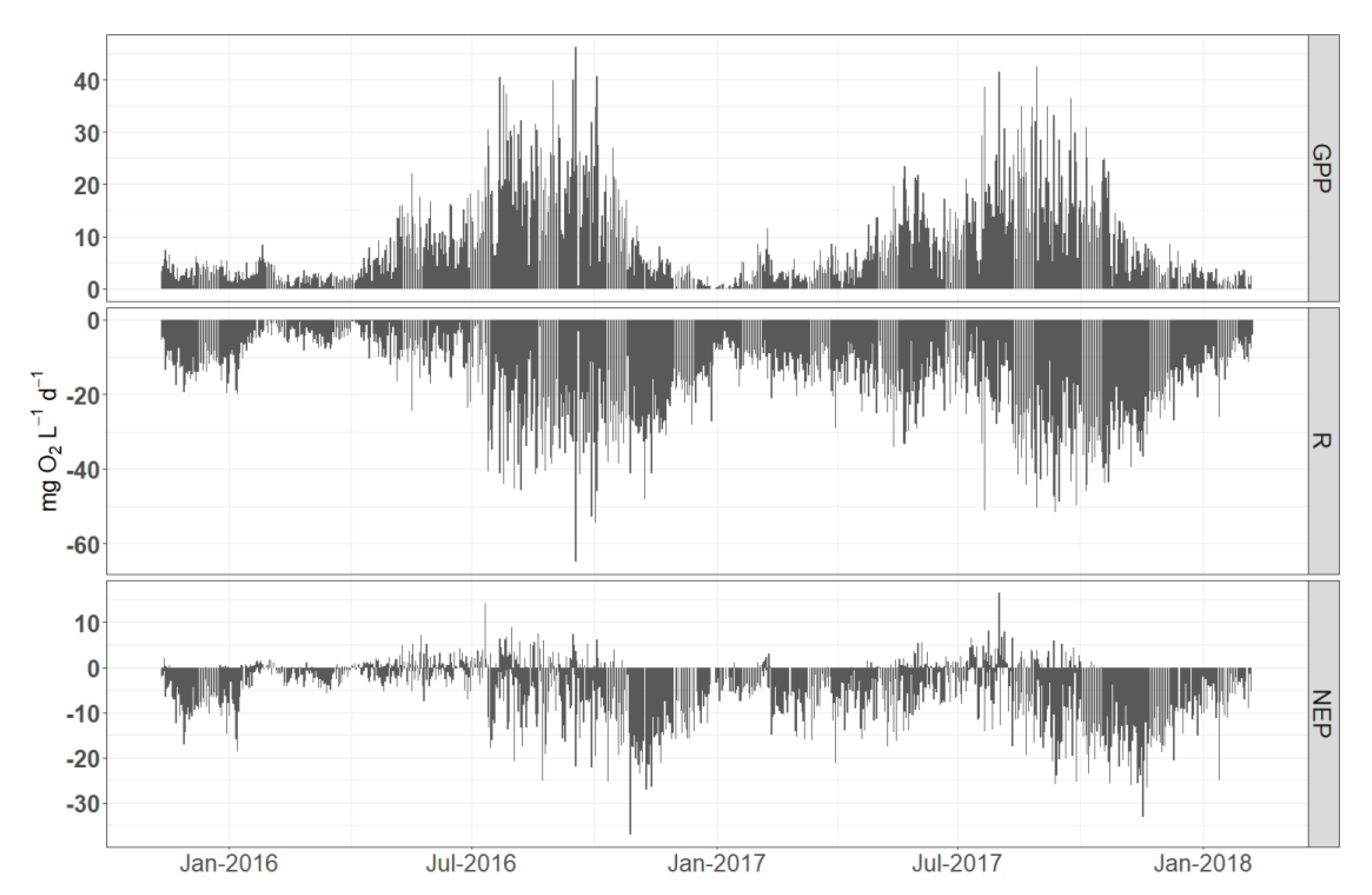
By further examining temporal trends on a daily time scale (Figure 7) it is obvious that higher metabolic activity occurs during summer months with high daily rates of respiration peaking during late autumn. In addition, NEP is predominantly heterotrophic with short periods of autotrophy noted during spring of 2016 and rarer in summer of 2017. Regardless, both monthly and daily timescales reveal the same trends, although aggregation of the daily estimates into monthly timescale smoothes extreme daily variations revealing clearer patterns.
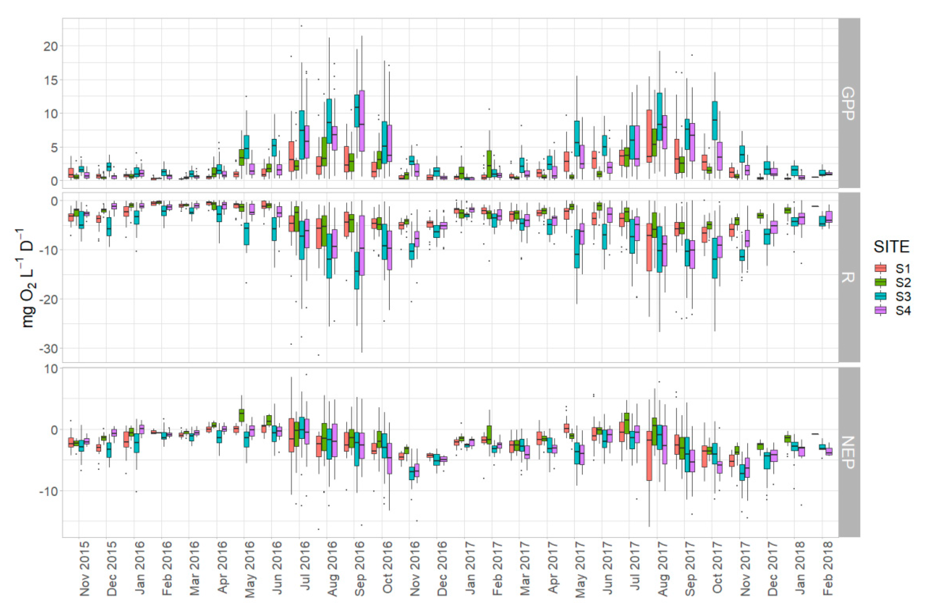
Regarding the temporal variation among sites, the rates of GPP and R in S3 and S4 showed larger variation than those for sites S1 and S2, particularly during the warm months of summer and early autumn (Figure 8). Furthermore, the monthly rates exceeded those of S3 and S4 for most of the duration of the study. Less obvious differences were observed in the monthly rates of NEP, with sites S3 and S4 being characterized by negative NEP rates for most of the studied period. Sites S1 and S2 showed mostly positive NEP rates during spring months of 2016, from April to June, when started to shift towards heterotrophy. In 2017 the metabolic balance in all the examined habitats was predominantly heterotrophic (mean NEP < 0).
3.3. Spatial Differences in Metabolic Estimates
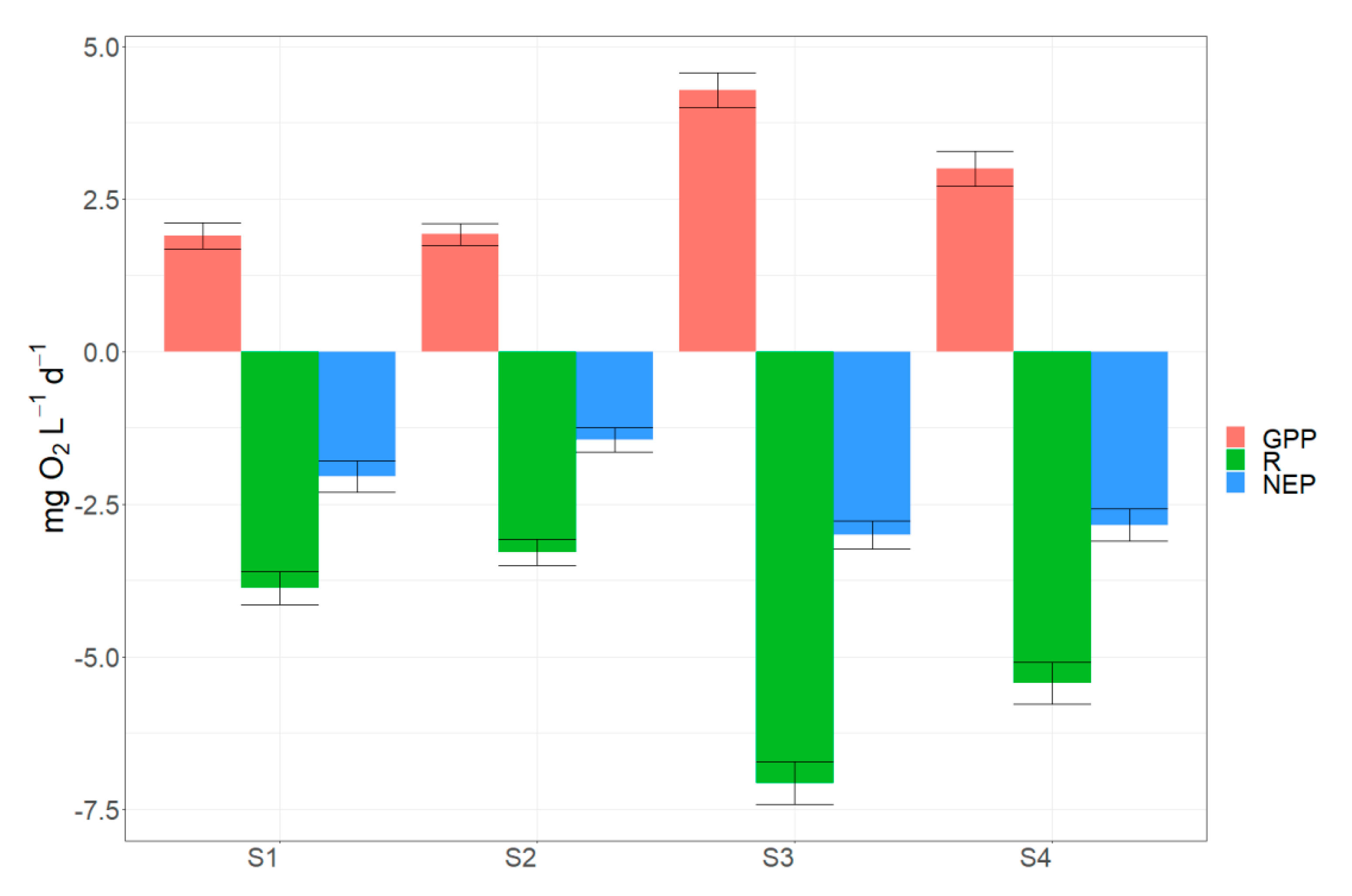
The results showed that GPP, R, and NEP rates calculated by pooled daily estimates for the study period differed significantly among the four monitoring stations (Figure 9). Mean rates of GPP were 1.90 and 1.92 mg L−1 d−1 O2 in sites S1 and S2 and 4.28 and 2.99 mg L−1 d−1 O2 in sites S3 and S4. A similar pattern was observed for mean R with S1 and S2 showing mean values of 3.84 and 3.28 mg L−1 d−1 O2 while S3 and S4 were characterized by significantly higher rates (7.07 and 5.43 mg L−1 d−1 O2 respectively). NEP presented lower differences among the sites varying from 2.04 mg L−1 d−1 O2 in site S1 to 3.00 mg L−1 d−1 O2 in site S3.
3.4. Exploring Relationships between Metabolic Estimates and Environmental Variables
Correlations between the metabolic estimates, abiotic variables, and chlorophyll-a concentration showed that rates of GPP, NEP and R were strongly related with temperature (both air and water), PAR and DO. Furthermore, GPP and NEP showed significant correlations with pH. Chlorophyll-a concentration correlated significantly with the metabolic estimates, but with lower coefficients. High correlations between GPP and NEP with R were also noted (Table 4).
The best linear models that were built using daily data (GPPd, Rd, NEPd in Table 5) showed as significant descriptors of GPPd (p < 0.001) the water temperature, PAR, wind speed, and conductivity, followed by Chl-a (p = 0.086). For Rd, PAR, water temperature and conductivity were significant model descriptors (p < 0.001). PAR, wind and Chl-a were primarily the most significant model parameters explaining the NEPd variation (p < 0.001) followed by conductivity (p = 0.039). Sites S3 and S4 also had a significant effect (p < 0.001) on GPP and R. In addition, R and NEP differed significantly between S2, S3, S4, and the S1. The pseudo-R2 value for the GPPd, Rd, and NEPd models were 0.544, 0.334 and 0.170 respectively (Table 5).
Concerning the models that were built with monthly data there were some obvious differences compared to the output of the “daily models”. The most significant predictors (p < 0.001) for the GPP model were the water temperature and wind speed (p < 0.001) followed by Chl-a (p = 0.112). Sites S3 and S4 differed significantly from the base level (site S1) as they were for the GPPd too. However, in contrast with the GPPd, PAR and conductivity were dropped during model selection process. On the contrary, the best Rm model showed the same predictors with the Rd (PAR, Wtr and EC) as the most important. The spatial effect was also very similar with the only difference the lower significance levels between S2, S4, and S1. The best NEPm was quite different from NEPd as only PAR and water temperature where the top predictors and wind speed was not significant (p = 0.069). An interesting result, compared to the NEPd model, is that the site did not had such an important effect on explaining the variation of monthly NEP as only S2 was found to differ significantly with S1. Finally, the pseudo-R2 values were 0.778, 0.606 and 0.401 for the GPPm, Rm, and NEPm respectively, suggesting that the “monthly” models explain larger portion of the total variance in the metabolic estimates.
4. Discussion
In this study, we estimated the spatiotemporal dynamics of metabolic estimates in four littoral sites with different characteristics in terms of surrounding landscape and dominant aquatic vegetation. Furthermore, we explored for key environmental factors that may control the variability in metabolism accounting for the localized influence of littoral habitats. It is worth noting that many studies have attempted to assess metabolic rates by using free-water measurements usually taken from a single site located at the pelagic zone of the lake without taking into account the metabolic rates in the shallow littoral. With this regard, our work can provide significant insight concerning metabolic dynamics in littoral habitats, yet due to lack of measurements from pelagic areas we cannot draw safe conclusions for the whole lake metabolism.
4.1. Daily vs. Monthly Variation in Metabolic Estimates
Estimations of aquatic metabolism always contain a significant amount of uncertainty associated with the measurements of DO concentrations, the quantification of air-water exchange and the spatial heterogeneity of oxygen dynamics [9,16,32,36]. In our case, daily metabolic estimates showed large variation, particularly during the summer months, that reflects not only the inherent uncertainty of metabolism estimation but also the dynamic behavior of shallow lake processes. Although large day-to-day variation is often attributed to methodological noise and uncertainty [14,37], there are also studies that underline the role of extreme climate events (storms and floods) in causing irregularities in metabolic dynamics [9]. Additionally, it was shown by Hanson et al. [38] that internal waves and other short-term mixing events (e.g., diurnal mixing phenomena) can affect the atmospheric flux of dissolved oxygen altering the metabolic estimates. It becomes obvious that there are several stochastic phenomena that can cause abrupt changes in the daily variation of metabolism which hinders our capability to explain the observed dynamics.
However, when the metabolic estimates were aggregated in monthly means our results showed more clearly the usual expected temporal trends that follow the seasonal variation of temperature and irradiance. This is also highlighted by Staehr et al. [9] in an extensive review where they reported that smoothing the high-frequency measurements would reduce uncertainties. In the same article the authors also recommended that a minimum measurement frequency of 1 hour is optimal for capturing the effects of short-term mixing events on dissolved oxygen, which complies with our monitoring strategy.
4.2. Spatial and Temporal Heterogeneity in Environmental Variables
All the investigated environmental parameters differed significantly among the four sites highlighting the spatial heterogeneity in water physicochemistry probably associated with the special local features and particularly the occurrence of aquatic vegetation in each habitat. Aquatic macrophytes are known to engineer their environment in various ways. For instance, Andersen et al. [39] showed that extensive coverage by charophytes in a shallow lake can influence the thermal regime and mechanical mixing within the lake. In this work, it was shown that regarding spatial variations in oxygen concentration the two sites S3 and S4, characterized by the dominance of the floating-leaved macrophyte Trapa natans, presented significantly lower concentrations than the sites with the submerged macrophytes. One possible explanation is related with the effects of floating-leaved mats of Trapa natans on the diurnal and seasonal dynamics of oxygen concentration [40,41,42]. These studies showed in particular that Trapa during summer develops large floating leaves forming dense mats that may promote larger oxygen depletion than the submerged vegetation. This could explain the lower oxygen concentrations measured in sites S3 and S4, although the differences were not as large as those marked by Caraco et al. [41], probably because Trapa in the studied lake formed less dense mats [25]. The occurrence of floating-leaved vegetation could also explain the lower concentration of chl-a due to shading effect creating poor light conditions that limit phytoplankton growth [43]. In an experimental study, De Tezanos Pinto et al. [44] showed that shading due to free-floating-leaved plants had a substantial effect on decreasing phytoplankton biomass and significantly lowering oxygen concentration causing hypoxia. Another likely explanation could be related with the agricultural runoffs at sites S1 and S2 that may have contributed into elevating phytoplankton biomass due to increased nutrient input. Furthermore, physicochemical conditions in S2 are likely to be influenced by flushing events (usually occurring during spring) that divert lake water to a nearby stream through a floodgate to manage high water levels.
4.3. Drivers of Temporal Variation in Metabolism
Our results showed that the temporal patterns of rates of GPP and R resembled those from other studies where the highest mean monthly values of GPP and R reached in late summer and the lowest in winter months [14,45,46]. This seasonal pattern was evidenced by the high dependency found between daily estimates of GPP, water temperature, and PAR. This agrees with the results for other shallow lakes (where seasonal patterns of GPP were driven by the temporal variations in water temperature and irradiance [14,22,45,46]). Besides, high summer temperatures can trigger high algal biomass that contributes to high rates of GPP [14]. However, in this study GPP showed weak correlation with algal biomass (chl-a) while both GPPd and GPPm models included chl-a as a non-significant predictor. This implies that high GPP rates in summer are driven by the growth of aquatic vegetation and periphyton in the littoral. The contribution of aquatic macrophytes in GPP was recently shown by Alfonso et al. [46] in a study of two eutrophic lakes with similar nutrient concentrations and contrasting submerged plant cover with the lake with abundant submerged plants presenting substantially higher GPP rates than the one with no macrophytes. Previous studies also had shown the significant effect of benthic vegetation in the metabolic processes by comparing vegetated littoral habitats with pelagic open water [18,19,47]. PAR and water temperature also were significant predictors for both Rd and Rm models which agrees with previous studies [14,22,46].
Regarding the temporal variation of the metabolic balance, it was shown that NEP inclined towards autotrophy during the spring months (April to June), when temperature and irradiance started to increase, but for the rest of the year it remained clearly heterotrophic. Positive monthly averages of NEP were observed only in site S2 from April to June of 2016. Higher negative rates of NEP were calculated during autumn (peak in November 2016 and 2017) when high respiration coincided with low productivity. This finding practically implies that respiration in autumn was predominantly fueled by decomposition of allochthonous organic material originated most likely from organics accumulated in the bottom following the highly productive summer months. This conclusion is further supported by a relatively moderate coupling we found between R and GPP. In general, a strong coupling between R and GPP indicates that respiration of autotrophs and heterotrophs relies on the autochthonous organic compounds that the autotrophs produce. The proportion of the GPP that is respired is estimated by models as high as approximately 80% and a slope of respiration on GPP between 0.8 and 1.0 usually reflects a high dependency of R on GPP [16]. In contrast, in highly eutrophic lakes the respiration-GPP coupling decreases substantially due to respiration of excessive production accumulated in the system [16,40]. In our case a slope of 0.77 of R on GPP suggests that respiration is likely fueled by allochthonous organic material, meaning either accumulated organics or inputs from the land–water interface, explaining the persistence of heterotrophy over longer periods. High contribution of allochthonous organic matter combined with favorable abiotic conditions enhance the growth of the heterotrophic community resulting in higher respiration rates than primary production [48]. In our case it is possible that the decayed aquatic plants in late autumn provide an additional source of organic matter that boosts the microbial respiration. Besides increasing respiration, input of allochthonous organic carbon into lake food webs has been shown to constrain productivity [49] by limiting light and nutrient availability further pushing metabolic balance to heterotrophy. It is very likely that the heterotrophic littoral greatly shapes the metabolic balance of the whole ecosystem shifting it towards heterotrophy even in the pelagic habitats. Although we do not have the evidence to support this statement, we know from the literature that aquatic metabolism in the littoral habitats is more dynamic and exhibits much larger metabolic rates than in pelagic [18,19]. This means, as Lauster et al. [18] suggested, that extensive littoral habitats would have a significant impact on the pelagic metabolism of shallow and small lakes. In addition, taking into account that there is a growing consensus that shallow productive and rich in dissolved organic carbon lakes are heterotrophic [16,48,50,51] we consider highly probable that the whole lake metabolism in our studied lake will be predominantly heterotrophic for most of the year.
4.4. Drivers of Spatial Heterogeneity in Metabolism
The studied habitats differed not only in their dissolved oxygen variability but also in the metabolic estimates (GPP and R) and their balance. Specifically, it was shown that GPP and R rates in sites S3 and S4 (Trapa natans dominance) were significantly higher than those in S1 and S2 (submerged vegetation beds). We consider more likely that these differences were due to the prevailing types of macrophyte vegetation. The contrasting role of floating-leaved vs submerged vegetation on water chemistry and plankton dynamics has been documented in numerous articles [24,52,53,54]. Yet, studies that have examined metabolic processes between areas with contrasting macrophyte life forms within the same lake are missing. There are a few examples from the literature that compare either metabolic rates between macrophyte stands from different lakes [18] or within the same river reach [40]. The study of Caraco and Cole [40] is more relevant with our case as it simulated NEP rates within a Trapa natans and a submerged vegetation bed and found substantially higher negative values for the Trapa natans bed which agrees with our observations. It is worth mentioning that Caraco and Cole attributed further variation in oxygen dynamics and metabolic rates to the size and the plant density of the Trapa bed explaining that in less dense macrophyte stands light can reach the submersed leaves of Trapa promoting high enough rates of GPP to offset the extremely large rates of R. This is probably the case in Lake Kastoria where less dense and even sporadic clusters of Trapa could explain why we did not record extremely low concentrations of DO and very low GPP rates.
There are other local factors that may have influenced the metabolic processes indirectly in the littoral. For instance, the surrounding landscape at both sites S1 and S2 is dominated by agricultures while S1 is additionally influenced by agricultural runoffs (originating mainly by orchards) that drain into ditches and streams that flow in the lake. This implies that agricultural runoffs may have a profound impact on nutrients and littoral communities affecting locally the metabolic rates. These effects were exemplified by Alfonso et al. [55] who documented that water inputs in a shallow lake in Argentina due to agricultural runoffs coincided with changes in nutrients and conductivity resulting in increased GPP and R rates. In our case however the observed pattern of spatial differences and the lack of additional information (e.g., nutrient concentrations and inflows) do not allow us to draw safe conclusions about the role of surrounding landuses and surface runoffs on the aquatic metabolism.
5. Conclusions
Our findings highlight the importance of interpreting metabolic rate measurements and temporal patterns of metabolic balance in littoral habitats of shallow lakes. In addition, this study underlines the importance of local-specific characteristics as drivers of productivity and respiration processes. In conclusion, we demonstrated that littoral habitats can exhibit dynamic temporal and spatial variability in metabolic estimates that is driven not only by water temperature and irradiance, but by local factors as well, such as the growth form of the prevailing aquatic vegetation. We also showed that the metabolic balance in the littoral was predominantly heterotrophic implying that a large portion of the lake acts as source of atmospheric carbon. Although we lack estimations of metabolism from pelagic areas, we consider very likely that the whole lake metabolism is greatly affected by the benthic communities in the littoral and thus it exhibits a heterotrophic metabolic state over large periods of the year. Consequently, we suggest that studies of metabolism in shallow lakes should take into account measurements with a wide distribution along the littoral spanning over large time scales to capture as much spatiotemporal variability as possible. Future research could focus on the effects of additional environmental factors and local management practices on the metabolic processes to enhance our understanding of the main drivers of metabolism in shallow lakes.
Author Contributions
Conceptualization, K.S.; methodology, K.S.; formal analysis, K.S.; investigation, K.S. and E.D.; resources, E.D.; data curation, K.S. and E.D.; writing—original draft preparation, K.S.; writing—review and editing, K.S. and E.D.; visualization, K.S.; project administration, E.D.; funding acquisition, E.D.
Funding
This research received no external funding.
Conflicts of Interest
The authors declare no conflict of interest.
References
- Odum, H.T. Primary Production in Flowing Waters. Limnol. Oceanogr. 1956, 1, 102–117. [Google Scholar] [CrossRef]
- Cole, J.J.; Prairie, Y.T.; Caraco, N.F.; McDowell, W.H.; Tranvik, L.J.; Striegl, R.G.; Duarte, C.M.; Kortelainen, P.; Downing, J.A.; Middelburg, J.J.; et al. Plumbing the global carbon cycle: Integrating inland waters into the terrestrial carbon budget. Ecosystems 2007, 10, 171–184. [Google Scholar] [CrossRef]
- Tranvik, L.J.; Cole, J.J.; Prairie, Y.T. The study of carbon in inland waters-from isolated ecosystems to players in the global carbon cycle. Limnol. Oceanogr. Lett. 2018, 3, 41–48. [Google Scholar] [CrossRef]
- Staehr, P.A.; Testa, J.M.; Kemp, W.M.; Cole, J.J.; Sand-Jensen, K.; Smith, S.V. The metabolism of aquatic ecosystems: History, applications, and future challenges. Aquat. Sci. 2012, 74, 15–29. [Google Scholar] [CrossRef]
- Tank, S.E.; Fellman, J.B.; Hood, E.; Kritzberg, E.S. Beyond respiration: Controls on lateral carbon fluxes across the terrestrial-aquatic interface. Limnol. Oceanogr. Lett. 2018, 3, 76–88. [Google Scholar] [CrossRef]
- Hanson, P.C.; Bade, D.L.; Carpenter, S.R.; Kratz, T.K. Lake metabolism: Relationships with dissolved organic carbon and phosphorus. Limnol. Oceanogr. 2003, 48, 1112–1119. [Google Scholar] [CrossRef]
- Hanson, P.C.; Carpenter, S.R.; Armstrong, D.E.; Stanley, E.H.; Kratz, T.K. Lake dissolved inorganic carbon and dissolved oxygen: Changing drivers from days to decades. Ecol. Monogr. 2006, 76, 343–363. [Google Scholar] [CrossRef]
- Brighenti, L.S.; Staehr, P.A.; Luciana, L.P.; Barbosa, F.A.R.; Bezerra-Neto, J.F. Importance of nutrients, organic matter and light availability on epilimnetic metabolic rates in a mesotrophic tropical lake. Freshw. Biol. 2018, 63, 1143–1160. [Google Scholar] [CrossRef]
- Staehr, P.A.; Bade, D.; van de Bogert, M.C.; Koch, G.R.; Williamson, C.; Hanson, P.; Cole, J.J.; Kratz, T. Lake metabolism and the diel oxygen technique: State of the science. Limnol. Oceanogr. Methods 2010, 8, 628–644. [Google Scholar] [CrossRef]
- Staehr, P.A.; Baastrup-Spohr, L.; Sand-Jensen, K.; Stedmon, C. Lake metabolism scales with lake morphometry and catchment conditions. Aquat. Sci. 2012, 74, 155–169. [Google Scholar] [CrossRef]
- Brighenti, L.S.; Staehr, P.A.; Gagliardi, L.M.; Brandão, L.P.M.; Elias, E.C.; de Mello, N.A.S.T.; Barbosa, F.A.R.; Bezerra-Neto, J.F. Seasonal Changes in Metabolic Rates of Two Tropical Lakes in the Atlantic Forest of Brazil. Ecosystems 2015, 18, 589–604. [Google Scholar] [CrossRef]
- Hotchkiss, E.R.; Sadro, S.; Hanson, P.C. Toward a more integrative perspective on carbon metabolism across lentic and lotic inland waters. Limnol. Oceanogr. Lett. 2018, 3, 57–63. [Google Scholar] [CrossRef]
- Seekell, D.A.; Lapierre, J.-F.; Cheruvelil, K.S. A geography of lake carbon cycling. Limnol. Oceanogr. Lett. 2018, 3, 49–56. [Google Scholar] [CrossRef]
- Staehr, P.A.; Sand-Jensen, K. Temporal dynamics and regulation of lake metabolism. Limnol. Oceanogr. 2007, 52, 108–120. [Google Scholar] [CrossRef]
- Laas, A.; Nõges, P.; Kõiv, T.; Nõges, T. High-frequency metabolism study in a large and shallow temperate lake reveals seasonal switching between net autotrophy and net heterotrophy. Hydrobiologia 2012, 694, 57–74. [Google Scholar] [CrossRef]
- Solomon, C.T.; Bruesewitz, D.A.; Richardson, D.C.; Rose, K.C.; Van de Bogert, M.C.; Hanson, P.C.; Kratz, T.K.; Larget, B.; Adrian, R.; Leroux Babin, B.; et al. Ecosystem respiration: Drivers of daily variability and background respiration in lakes around the globe. Limnol. Oceanogr. 2013, 58, 849–866. [Google Scholar] [CrossRef]
- Van de Bogert, M.C.; Bade, D.L.; Carpenter, S.R.; Cole, J.J.; Pace, M.L.; Hanson, P.C.; Langman, O.C. Spatial heterogeneity strongly affects estimates of ecosystem metabolism in two north temperate lakes. Limnol. Oceanogr. 2012, 57, 1689–1700. [Google Scholar] [CrossRef]
- Lauster, G.H.; Hanson, P.C.; Kratz, T.K. Gross primary production and respiration differences among littoral and pelagic habitats in northern Wisconsin lakes. Can. J. Fish. Aquat. Sci. 2006, 63, 1130–1141. [Google Scholar] [CrossRef]
- Van de Bogert, M.C.; Carpenter, S.R.; Cole, J.J.; Pace, M.L. Assessing pelagic and benthic metabolism using free water measurements. Limnol. Oceanogr. Methods 2007, 5, 145–155. [Google Scholar] [CrossRef]
- Sadro, S.; Melack, J.M.; MacIntyre, S. Spatial and Temporal Variability in the Ecosystem Metabolism of a High-elevation Lake: Integrating Benthic and Pelagic Habitats. Ecosystems 2011, 14, 1123–1140. [Google Scholar] [CrossRef]
- Vesterinen, J.; Devlin, S.P.; Syväranta, J.; Jones, R.I. Influence of littoral periphyton on whole-lake metabolism relates to littoral vegetation in humic lakes. Ecology 2017, 98, 3074–3085. [Google Scholar] [CrossRef] [PubMed]
- Idrizaj, A.; Laas, A.; Anijalg, U.; Nõges, P. Horizontal differences in ecosystem metabolism of a large shallow lake. J. Hydrol. 2016, 535, 93–100. [Google Scholar] [CrossRef]
- Moustaka-Gouni, M.; Vardaka, E.; Michaloudi, E.; Kormas, K.A.; Tryfon, E.; Mihalatou, H.; Gkelis, S.; Lanaras, T. Plankton food web structure in a eutrophic polymictic lake with a history in toxic cyanobacterial blooms. Limnol. Oceanogr. 2006, 51, 715–727. [Google Scholar] [CrossRef]
- Stefanidis, K.; Papastergiadou, E. Influence of hydrophyte abundance on the spatial distribution of zooplankton in selected lakes in Greece. Hydrobiologia 2010, 656, 55–65. [Google Scholar] [CrossRef]
- Stefanidis, K. Ecological Assessment of Lakes of NW Greece with Emphasis on the Associations between Aquatic Macrophytes, Zooplankton and Water Quality. Ph.D. Thesis, Department of Biology, University of Patras, Patras, Greece, 2012. [Google Scholar] [CrossRef]
- Stefanidis, K.; Papastergiadou, E. Relationships between lake morphometry, water quality and aquatic macrophytes in Greek lakes. Fresenius Environ. Bull. 2012, 21, 3018–3026. [Google Scholar]
- Moustaka-Gouni, M.; Vardaka, E.; Tryfon, E. Phytoplankton species succession in a shallow Mediterranean lake (L. Kastoria, Greece): Steady-state dominance of Limnothrixredekei, Microcystis aeruginosa and Cylindrospermopsisraciborskii. Hydrobiologia 2007, 575, 129–140. [Google Scholar] [CrossRef]
- Latinopoulos, D.; Ntislidou, C.; Kagalou, I. A multi-approach Lake Habitat Survey method for impact assessment in two heavily modified lakes: A case of two Northern Greek lakes. Environ. Monit. Assess. 2018, 190, 658. [Google Scholar] [CrossRef] [PubMed]
- Winslow, L.A.; Zwart, J.A.; Batt, R.D.; Dugan, H.A.; Iestyn Woolway, R.; Corman, J.R.; Hanson, P.C.; Read, J.S. LakeMetabolizer: An R package for estimating lake metabolism from free-water oxygen using diverse statistical models. InlandWaters 2016, 6, 622–636. [Google Scholar] [CrossRef]
- Woolway, R.I.; Jones, I.D.; Hamilton, D.P.; Maberly, S.C.; Muraoka, K.; Read, J.S.; Smyth, R.L.; Winslow, L.A. Automated calculation of surface energy fluxes with high-frequency lake buoy data. Environ. Model. Softw. 2015, 70, 191–198. [Google Scholar] [CrossRef]
- Vachon, D.; Prairie, Y.T. The ecosystem size and shape dependence of gas transfer velocity versus wind speed relationships in lakes. Can. J. Fish. Aquat. Sci. 2013, 70, 1757–1764. [Google Scholar] [CrossRef]
- Dugan, H.A.; Iestyn Woolway, R.; Santoso, A.B.; Corman, J.R.; Jaimes, A.; Nodine, E.R.; Patil, V.P.; Zwart, J.A.; Brentrup, J.A.; Hetherington, A.L.; et al. Consequences of gas flux model choice on the interpretation of metabolic balance across 15 lakes. InlandWaters 2016, 6, 581–592. [Google Scholar] [CrossRef]
- Batt, R.D.; Carpenter, S.R. Free-water lake metabolism: Addressing noisy time series with a Kalman filter. Limnol. Oceanogr. Methods 2012, 10, 20–30. [Google Scholar] [CrossRef]
- R Core Team. R: A Language and Environment for Statistical Computing; R Foundation for Statistical Computing: Vienna, Austria, 2018. [Google Scholar]
- Bartón, K. MuMIn: Multi-Model Inference. R Package Version 1.15.6. 2016. Available online: https://CRAN.R-project.org/package=MuMIn (accessed on 18 November 2018).
- Rose, K.C.; Winslow, L.A.; Read, J.S.; Read, E.K.; Solomon, C.T.; Adrian, R.; Hanson, P.C. Improving the precision of lake ecosystem metabolism estimates by identifying predictors of model uncertainty. Limnol. Oceanogr. Methods 2014, 12, 303–312. [Google Scholar] [CrossRef]
- Cremona, F.; Laas, A.; Nõges, P.; Nõges, T. An estimation of diel metabolic rates of eight limnological archetypes from Estonia using high-frequency measurements. InlandWaters 2016, 6, 352–363. [Google Scholar] [CrossRef]
- Hanson, P.C.; Carpenter, S.R.; Kimura, N.; Wu, C.; Cornelius, S.P.; Kratz, T.K. Evaluation of metabolism models for free-water dissolved oxygen methods in lakes. Limnol. Oceanogr. Methods 2008, 6, 454–465. [Google Scholar] [CrossRef]
- Andersen, M.R.; Sand-Jensen, K.; Woolway, R.I.; Jones, I.D. Profound daily vertical stratification and mixing in a small, shallow, wind-exposed lake with submerged macrophytes. Aquat. Sci. 2017, 79, 395–406. [Google Scholar] [CrossRef]
- Caraco, N.F.; Cole, J.J. Contrasting impacts of a native and alien macrophyte on dissolved oxygen in a large river. Ecol. Appl. 2002, 12, 1496–1509. [Google Scholar] [CrossRef]
- Caraco, N.; Cole, J.; Findlay, S.; Wigand, C. Vascular Plants as Engineers of Oxygen in Aquatic Systems. Bioscience 2006, 56, 219. [Google Scholar] [CrossRef]
- Goodwin, K.; Caraco, N.; Cole, J. Temporal dynamics of dissolved oxygen in a floating-leaved macrophyte bed. Freshw. Biol. 2008, 53, 1632–1641. [Google Scholar] [CrossRef]
- Yamaki, A.; Yamamuro, M. Floating-leaved and emergent vegetation as habitat for fishes in a eutrophic temperate lake without submerged vegetation. Limnology 2013, 14, 257–268. [Google Scholar] [CrossRef]
- De Tezanos Pinto, P.; Allende, L.; O’Farrell, I. Influence of free-floating plants on the structure of a natural phytoplankton assemblage: An experimental approach. J. Plankton Res. 2007, 29, 47–56. [Google Scholar] [CrossRef]
- Staehr, P.A.; Christensen, J.P.A.; Batt, R.D.; Read, J.S. Ecosystem metabolism in a stratified lake. Limnol. Oceanogr. 2012, 57, 1317–1330. [Google Scholar] [CrossRef]
- Alfonso, M.; Brendel, A.; Vitale, A.; Seitz, C.; Piccolo, M.; Perillo, G. Drivers of Ecosystem Metabolism in Two Managed Shallow Lakes with Different Salinity and Trophic Conditions: The Sauce Grande and La Salada Lakes (Argentina). Water 2018, 10, 1136. [Google Scholar] [CrossRef]
- Pinardi, M.; Bartoli, M.; Longhi, D.; Viaroli, P. Net autotrophy in a fluvial lake: The relative role of phytoplankton and floating-leaved macrophytes. Aquat. Sci. 2011, 73, 389–403. [Google Scholar] [CrossRef]
- Cole, J.J.; Pace, M.L.; Carpenter, S.R.; Kitchell, J.F. Persistence of net heterotrophy in lakes during nutrient addition and food web manipulations. Limnol. Oceanogr. 2000, 45, 1718–1730. [Google Scholar] [CrossRef]
- Karlsson, J.; Byström, P.; Ask, J.; Ask, P.; Persson, L.; Jansson, M. Light limitation of nutrient-poor lake ecosystems. Nature 2009, 460, 506–509. [Google Scholar] [CrossRef] [PubMed]
- Duarte, C.M.; Prairie, Y.T. Prevalence of heterotrophy and atmospheric CO2 emissions from aquatic ecosystems. Ecosystems 2005, 8, 862–870. [Google Scholar] [CrossRef]
- Hoellein, T.J.; Bruesewitz, D.A.; Richardson, D.C. Revisiting Odum (1956): A synthesis of aquatic ecosystem metabolism. Limnol. Oceanogr. 2013, 58, 2089–2100. [Google Scholar] [CrossRef]
- Horppila, J.; Nurminen, L. Effects of different macrophyte growth forms on sediment and P resuspension in a shallow lake. Hydrobiologia 2005, 545, 167–175. [Google Scholar] [CrossRef]
- Kuczyńska-Kippen, N.M.; Nagengast, B. The influence of the spatial structure of hydromacrophytes and differentiating habitat on the structure of rotifer and cladoceran communities. Hydrobiologia 2006, 559, 203–212. [Google Scholar] [CrossRef]
- Holmroos, H.; Horppila, J.; Niemistö, J.; Nurminen, L.; Hietanen, S. Dynamics of dissolved nutrients among different macrophyte stands in a shallow lake. Limnology 2014, 16, 31–39. [Google Scholar] [CrossRef]
- Alfonso, M.B.; Vitale, A.J.; Menéndez, M.C.; Perillo, V.L.; Piccolo, M.C.; Perillo, G.M.E. Estimation of ecosystem metabolism from diel oxygen technique in a saline shallow lake: La Salada (Argentina). Hydrobiologia 2015, 752, 223–237. [Google Scholar] [CrossRef]
Figure 1.
Map showing the location of the monitoring sites in the lake, the distribution of land uses within the basin and major inflow and outflow streams.
Figure 1.
Map showing the location of the monitoring sites in the lake, the distribution of land uses within the basin and major inflow and outflow streams.

Figure 2.
Monthly means (pooled samples) of chlorophyll-a concentration (Chl-a), electrical conductivity (EC), dissolved oxygen concentration (DO) and pH. Error bars indicate standard error (SE).
Figure 2.
Monthly means (pooled samples) of chlorophyll-a concentration (Chl-a), electrical conductivity (EC), dissolved oxygen concentration (DO) and pH. Error bars indicate standard error (SE).

Figure 3.
Monthly trends in chlorophyll-a concentration (Chl-a), electrical conductivity (EC), dissolved oxygen concentration (DO) and pH per site.
Figure 3.
Monthly trends in chlorophyll-a concentration (Chl-a), electrical conductivity (EC), dissolved oxygen concentration (DO) and pH per site.

Figure 4.
Means of chlorophyll-a concentration (Chl-a), dissolved oxygen concentration (DO), electrical conductivity (EC) and pH among the four monitoring sites/littoral habitats. Error bars indicate standard errors (SE).
Figure 4.
Means of chlorophyll-a concentration (Chl-a), dissolved oxygen concentration (DO), electrical conductivity (EC) and pH among the four monitoring sites/littoral habitats. Error bars indicate standard errors (SE).

Figure 5.
Daily variation of meteorological variables (from top to bottom: Wind speed, PAR, relative humidity, air temperature).
Figure 5.
Daily variation of meteorological variables (from top to bottom: Wind speed, PAR, relative humidity, air temperature).

Figure 6.
Boxplots of calculated GPP, R, and NEP from pooled measurements (all sites included) showing the temporal variation.
Figure 6.
Boxplots of calculated GPP, R, and NEP from pooled measurements (all sites included) showing the temporal variation.

Figure 7.
Daily variations of metabolic estimates calculated from pooled measurements (all sites included). Missing values are due to exclusion of impossible estimates, e.g., negative GPP or positive R.
Figure 7.
Daily variations of metabolic estimates calculated from pooled measurements (all sites included). Missing values are due to exclusion of impossible estimates, e.g., negative GPP or positive R.

Figure 8.
Boxplots of calculated metabolic estimates (GPP, R, and NEP) for each site showing the temporal variation.
Figure 8.
Boxplots of calculated metabolic estimates (GPP, R, and NEP) for each site showing the temporal variation.

Figure 9.
Mean values of metabolic estimates (GPP, R, and NEP) per each site. Error bars indicate standard error.
Figure 9.
Mean values of metabolic estimates (GPP, R, and NEP) per each site. Error bars indicate standard error.


Table 1.
Basic information on the studied lake.
| Lake Information | Value | Source |
|---|---|---|
| Latitude | 40°31′ N | [23] |
| Longitude | 21°18′ E | |
| Altitude (m) | 629 | |
| Retention time (years) | >2 | |
| Mean depth (m) | 4.4 | [24] |
| Max. depth (m) | 9 | |
| Surface (km2) | 28 | |
| Average phosphorus concentration (mg L−1) | 0.2 | [26] |
| Average dissolved inorganic nitrogen concentration (mg L−1) | 0.27 | |
| Average chlorophyll-a concentration (μg L−1) | 15.90 | |
| Aquatic vegetation (most common species) | Trapa natans, Myriophyllum spicatum, Ceratophyllum demersum | [25,26] |
Table 2.
Characteristics of littoral habitats with respect to dominant aquatic vegetation, land uses, and lakeshore morphological alterations.
Table 2.
Characteristics of littoral habitats with respect to dominant aquatic vegetation, land uses, and lakeshore morphological alterations.
| Site | Aquatic Vegetation | Adjacent Land Use | Lakeshore Morphological Alterations |
|---|---|---|---|
| S1 | Submerged vegetation (Myriophyllum spicatum, Ceratophyllum demersum) | Agricultures | Low–Moderate |
| S2 | Agricultures | Moderate | |
| S3 | Floating-leaved vegetation (Trapa natans) | Urbanized land uses | High High |
| S4 | Floating-leaved vegetation (Trapa natans) | Urbanized land uses |
Table 3.
Parameters recorded by the sondes and the meteorological station.
| Parameter | Abbreviation | Frequency of Measurement |
|---|---|---|
| Concentration of dissolved oxygen (mg L−1) | DO | 1 h |
| Water temperature (°C) | Wtr | 1 h |
| Air temperature (°C) | airT | 10 min |
| Wind speed at 10 m height (m s−1) | wnd | 10 min |
| Photosynthetically active radiation (W m−2) | irr | 10 min |
| Relative humidity (%) | rh | 10 min |
| pH | pH | 1 h |
| Electrical conductivity (μS cm−1) | cond | 1 h |
| Chlorophyll-a (μg L−1) | chl-a | 1 h |
Table 4.
Pearson correlation coefficients between daily estimates of gross (GPP) and net (NEP) ecosystem production, respiration (R), daily mean wind speed at 10 m above surface (wind), relative humidity (Rh), daily mean photosynthetically active radiation (PAR), daily mean air temperature (AirT.), daily mean chlorophyll-a concentration, daily mean electrical conductivity (EC), daily mean dissolved oxygen concentration (DO), daily mean pH and daily mean water temperature (Wtr.). ** indicates significance level p < 0.001 and * significance p < 0.05.
| GPP | R | NEP | Wnd | Rh | PAR | AirT. | Chl-a | EC | DO | pH | |
|---|---|---|---|---|---|---|---|---|---|---|---|
| R | −0.77 ** | 1 | |||||||||
| NEP | 0.04 | 0.61 ** | 1 | ||||||||
| Wnd | −0.13 ** | 0.04 * | −0.1 ** | 1 | |||||||
| Rh | −0.27 ** | 0.09 ** | −0.19 ** | −0.17 ** | 1 | ||||||
| PAR | 0.38 ** | −0.11 ** | 0.29 ** | 0.07 | −0.77 ** | 1 | |||||
| AirT. | 0.48 ** | −0.25 ** | 0.2 ** | 0.05 | −0.47 ** | 0.67 ** | 1 | ||||
| Chl-a | −0.08 ** | 0.14 ** | 0.12 ** | −0.05 | 0.08 * | −0.09 | −0.07 | 1 | |||
| EC | −0.17 ** | 0.13 ** | −0.01 | 0.2 ** | −0.15 ** | 0.18 ** | −0.05 ** | −0.14 ** | 1 | ||
| DO | −0.22 ** | 0.51 ** | 0.52 ** | 0.08 ** | 0.07 | −0.1 ** | −0.25 ** | 0.16 ** | −0.01 | 1 | |
| pH | 0.4 ** | −0.1 ** | 0.33 ** | 0.03 | −0.23 ** | 0.39 ** | 0.52 ** | 0.1 ** | −0.25 ** | 0.19 ** | 1 |
| Wtr. | 0.53 ** | −0.31 ** | 0.17 ** | −0.01 ** | −0.45 ** | 0.7 ** | 0.91 ** | −0.07 | −0.06 ** | −0.35 ** | 0.54 ** |
Table 5.
Linear models of GPP, R, and NEP as function of wind speed at 10 m above surface (Wnd), photosynthetically active radiation (PAR), chlorophyll-a concentration (Chl-a), electrical conductivity (EC), water temperature (Wtr.) and site. (* The suffix d refers to model built with daily data and m refers to model built with monthly means).
| Dependent Variable | Parameter | Pseudo—R2 | Coefficient | p |
|---|---|---|---|---|
| Daily time scale | ||||
| GPPd | (intercept) | 0.544 | −0.304 | p < 0.001 |
| Wtr. | 0.407 | p < 0.001 | ||
| PAR | 0.211 | p < 0.001 | ||
| Wnd | 0.019 | p < 0.001 | ||
| EC | 0.021 | p < 0.001 | ||
| Chl-a | −0.035 | p = 0.086 | ||
| S2 | −0.072 | p = 0.148 | ||
| S3 | 0.839 | p < 0.001 | ||
| S4 | 0.548 | p < 0.001 | ||
| Rd | (intercept) | 0.334 | 0.252 | p < 0.001 |
| PAR | 0.111 | p < 0.001 | ||
| Wtr. | −0.292 | p < 0.001 | ||
| EC | 0.240 | p < 0.001 | ||
| S2 | 0.303 | p < 0.001 | ||
| S3 | −0.846 | p < 0.001 | ||
| S4 | −0.623 | p < 0.001 | ||
| NEPd | (intercept) | 0.170 | 0.003 | p = 0.946 |
| PAR | 0.342 | p < 0.001 | ||
| Wnd | −0.085 | p < 0.001 | ||
| Chl-a | 0.095 | p < 0.001 | ||
| EC | 0.055 | p = 0.039 | ||
| S2 | 0.291 | p < 0.001 | ||
| S3 | −0.201 | p = 0.006 | ||
| S4 | −0.189 | p = 0.010 | ||
| Monthly time scale | ||||
| GPPm | (intercept) | 0.778 | −0.391 | p = 0.001 |
| Wnd | −0.180 | p < 0.001 | ||
| Wtr. | 0.698 | p < 0.001 | ||
| Chl-a | 0.101 | p = 0.112 | ||
| S2 | −0.003 | p = 0.984 | ||
| S3 | 1.067 | p < 0.001 | ||
| S4 | 0.444 | p = 0.005 | ||
| Rm | (intercept) | 0.606 | 0.211 | p = 0.052 |
| Wtr. | −0.988 | p < 0.001 | ||
| PAR | 0.679 | p < 0.001 | ||
| EC | 0.147 | p = 0.052 | ||
| S2 | 0.384 | p = 0.050 | ||
| S3 | −0.943 | p < 0.001 | ||
| S4 | −0.452 | p = 0.021 | ||
| NEPm | (intercept) | 0.401 | −0.007 | p = 0.965 |
| PAR | 1.134 | p < 0.001 | ||
| Wtr. | −0.774 | p < 0.001 | ||
| Wnd | −0.206 | p = 0.069 | ||
| S2 | 0.569 | p = 0.013 | ||
| S3 | −0.314 | p = 0.165 | ||
| S4 | −0.206 | p = 0.361 |
© 2019 by the author. Licensee MDPI, Basel, Switzerland. This article is an open access article distributed under the terms and conditions of the Creative Commons Attribution (CC BY) license (http://creativecommons.org/licenses/by/4.0/).
Share and Cite
MDPI and ACS Style
Stefanidis, K.; Dimitriou, E. Differentiation in Aquatic Metabolism between Littoral Habitats with Floating-Leaved and Submerged Macrophyte Growth Forms in a Shallow Eutrophic Lake. Water 2019, 11, 287. https://doi.org/10.3390/w11020287
AMA Style
Stefanidis K, Dimitriou E. Differentiation in Aquatic Metabolism between Littoral Habitats with Floating-Leaved and Submerged Macrophyte Growth Forms in a Shallow Eutrophic Lake. Water. 2019; 11(2):287. https://doi.org/10.3390/w11020287
Chicago/Turabian StyleStefanidis, Konstantinos, and Elias Dimitriou. 2019. "Differentiation in Aquatic Metabolism between Littoral Habitats with Floating-Leaved and Submerged Macrophyte Growth Forms in a Shallow Eutrophic Lake" Water 11, no. 2: 287. https://doi.org/10.3390/w11020287
Note that from the first issue of 2016, this journal uses article numbers instead of page numbers. See further details here.