Including Variability across Climate Change Projections in Assessing Impacts on Water Resources in an Intensively Managed Landscape


1
Natural Resources and Environmental Management, Ball State University, Muncie, IN 47304, USA
2
Geosciences, Boise State University, Boise, ID 83725, USA
3
Human-Environment Systems, Boise State University, Boise, ID 83725, USA
*
Authors to whom correspondence should be addressed.
Water 2019, 11(2), 286; https://doi.org/10.3390/w11020286
Submission received: 3 January 2019
/
Revised: 24 January 2019
/
Accepted: 2 February 2019
/
Published: 6 February 2019
(This article belongs to the Section Hydrology)
Abstract
:Key Points
- Parameters of a stochastic weather generator are estimated from 11 bias-corrected simulations of two Representative Concentration Pathways (RCPs) 4.5 and 8.5, and weather observations of the recent past.
- We generate one hundred realizations of daily weather for RCP 4.5, RCP 8.5, and ten recent past (PAST) scenarios and input them into a model capturing natural hydrology and water management in an intensively managed system.
- Model outputs allow us to quantify probability distributions of allocated and unsatisfied irrigation water and their spatial patterns and indicate that warmer scenarios are associated with higher and more variable unsatisfied demand.
Abstract
In intensively managed watersheds, water scarcity is a product of interactions between complex biophysical processes and human activities. Understanding how intensively managed watersheds respond to climate change requires modeling these coupled processes. One challenge in assessing the response of these watersheds to climate change lies in adequately capturing the trends and variability of future climates. Here we combine a stochastic weather generator together with future projections of climate change to efficiently create a large ensemble of daily weather for three climate scenarios, reflecting recent past and two future climate scenarios. With a previously developed model that captures rainfall-runoff processes and the redistribution of water according to declared water rights, we use these large ensembles to evaluate how future climate change may impact satisfied and unsatisfied irrigation throughout the study area, the Treasure Valley in Southwest Idaho, USA. The numerical experiments quantify the changing rate of allocated and unsatisfied irrigation amount and reveal that the projected temperature increase more significantly influences allocated and unsatisfied irrigation amounts than precipitation changes. The scenarios identify spatially distinct regions in the study area that are at greater risk of the occurrence of unsatisfied irrigation. This study demonstrates how combining stochastic weather generators and future climate projections can support efforts to assess future risks of negative water resource outcomes. It also allows identification of regions in the study area that may be less suitable for irrigated agriculture in future decades, potentially benefiting planners and managers.
1. Introduction
Changes to precipitation and temperature regimes associated with global warming pose a particular challenge to intensively managed watersheds because of changes in climate impact both water supply and demand. A significant body of work has sought to characterize the impacts of climate change on water supply through, for instance, quantifying changes in precipitation, snowpack dynamics, and runoff [1,2,3]. The anticipation of future climate by analysis of water uses can also influence decision-making that directly impacts water use through, for example, crop choice, irrigation practices, crop rotation, and land use [4].
At the same time, considerable uncertainties in climate projections exist due to the internal variability of the climate system, equations used in different general circulation models, and the design of scenarios [5]. The wide spread of the future projections of precipitation and temperature, particularly at regional scales, introduce difficulties in characterizing the impacts of climate change in intensively managed systems. To address some of these uncertainties induced by model spread, it is becoming increasingly common to use the downscaled output of multiple General Circulation Model (GCM) simulations to capture a broader range of potential climate change outcomes [6]. Currently available downscaled datasets used for climate change impact studies at regional scales, however, may not adequately capture uncertainties within climate models in ways that can support robust quantification of the uncertainties in important outcomes like insufficiencies in the water supply.
Large ensembles of potential future climate that capture both within and between GCM variability would substantially aid in assessing the impacts of climate change in intensively managed systems. But developing large forcing ensembles for statistical and/or dynamical downscaling [7,8] can be prohibitively expensive in terms of computational and data storage requirements.
Stochastic weather generators represent a potentially useful tool for developing environmental forces required as input to hydrological models in ways that address the challenges outlined above. These tools were developed to create plausible realizations of weather variables (e.g., temperature, precipitation, humidity) when only climatic statistics are available [9,10,11,12,13]. Although they rely on a number of simplifying assumptions, they can efficiently create large ensembles of forcing realizations on climate variables. One significant limitation, however, is that stochastic weather generators rely on stationarity in climate processes captured by the statistics used to generate realizations of weather. Additionally, since the output of a stochastic weather generator is one draw of a stochastic process, it is necessary to (1) generate an ensemble of realizations of weather, (2) use this ensemble to create a corresponding ensemble of environmental outcomes by supplying each weather realization as input to an environmental model, and (3) examine the probabilistic structure across all outcomes.
Here we develop and apply a framework for combining statistically downscaled outputs from multiple GCMs with a stochastic weather generator to quantify the impacts of climate change on a coupled socio-hydrologic system in a probabilistic fashion. Using a combination of GCM output and stochastic weather generators has previously been used to examine the hydrological and ecological impacts of climate change [12,14]. These previous studies, however, relied on output from only one GCM projection, thereby neglecting uncertainties associated with the spectrum of GCMs currently used for global climate change analysis as part of the Intergovernmental Panel on Climate Change (IPCC) quadrennial review. We extend these efforts by developing techniques to use information from multiple GCMs together with an existing stochastic weather generator to produce large ensembles of daily weather variables required as inputs to many environmental models. The method uses statistically downscaled outputs from multiple GCMs to derive empirical probability distribution functions of key statistics required as inputs to the stochastic weather generator. The climate statistics required as inputs to the stochastic weather generator are then drawn at random from these empirical density functions and a realization of daily weather variables created. This process is repeated to create a large ensemble of realizations of daily weather required as inputs to a model of the coupled human-hydrological system in the study area. In this way, uncertainty across the spectrum of GCMs is accounted for by treating the climate statistics required as inputs to the weather generator as uncertain themselves.
We apply generated forcing ensembles to examine the potential ramifications of climate change in a coupled human-natural systems model in an intensively irrigated, semi-arid watershed. In particular, the coupled model simulates both biophysical hydrological processes, as well as redistribution of water in accordance with the spatiotemporal regime of water rights operating in the region. By using this large forcing ensemble to create a corresponding ensemble of climate impacts, we can examine both the average and variability in both future water use and unsatisfied demand. We examined outcomes in this system under three climate scenarios: (1) A baseline scenario reflecting the recent past (PAST), (2) the IPCC Representative Concentration Pathway (RCP) 4.5 scenario (RCP4.5), and (3) the IPCC RCP 8.5 scenario (RCP8.5). An outcome of particular value is the insight into the spatial and temporal distribution of disruptions to water supply predicted by the simulations. The average annual allocated irrigation water in the RCP4.5 and RCP8.5 scenario groups is 20.5% and 32.5% higher than that in the PAST scenario group. Similarly, the mean value of the unsatisfied water increases by 57.1% and 147.6% in comparison with the PAST scenario. The conducted simulations are at a spatiotemporal scale that is of value to stakeholders in planning for and adapting water resources in the region to a changing climate. In particular, our simulations help to identify regions in the study area more prone to insufficient water supplies in future decades because of the compounding effects of changes in precipitation and temperature regimes on one hand, and unfavorable water rights seniority on the other. What follows is a description of the methodological approach and experimental setup, a summary of relevant results, and a discussion of potential implications, limitations, and extensions of this work.
2. Study Area
The study site corresponds to the Lower Boise River Basin, also known as the Treasure Valley, in Southwest Idaho, USA (Figure 1). The region is the most populous and rapidly growing area within the state and serves as a natural laboratory for studying ongoing challenges associated with population growth, urbanization, agricultural production, and climate and hydrologic change. The watershed has a total area of 3323 km2. The climate in the Treasure Valley is generally consistent with a semi-arid Mediterranean climate with hot, dry summers (average temperature of 32.8 °C in July; average precipitation of 6.1 mm in August) and cold, wet winters (average temperature of −3.9 °C in January; average precipitation of 39 mm in January). Annual rainfall varies substantially in space within the basin, from ~700 mm in the Northeast foothills to ~200 mm in the Southwest, with a long-term observed average of about 296 mm/yr at Boise Air Terminal weather station. Elevation of the watershed ranges from 662 m to 1989 m. In the absence of agricultural and developed land uses, vegetation cover in the region is consistent with the Sagebrush-steppe ecosystem of the larger Great Basin ecoregion. Importantly, the Treasure Valley is home to Idaho’s three largest cities (Boise, Meridian, and Nampa). The population of the Boise City-Nampa Metropolitan Statistical Area (MSA) was 709,845 as of 2017, up from 616,561 in the 2010 Census, an average annual increase of 2.03%. Thus, the Treasure Valley region is being subject to significant land use conversion, resulting in changes to biophysical and social systems, and interactions between the two.
Climate exerts a significant control over the use of water resources within the region. More than half of the total precipitation that falls within the Treasure Valley, which is not sufficient to support many high-value crops, occurs during the non-irrigation season. As such, local agriculture relies heavily on irrigation water from the Upper Boise River Basin (UBRB), particularly during the hot, dry portion of the growing season. Climate change driven increase in temperatures in the Treasure Valley not only increases atmospheric water demand during the growing season, but also impacts of climate change shifts the timing, amount, and phase of precipitation that will lead to earlier runoff and increased variability from the UBRB.
Irrigation is facilitated by a series of reservoirs upstream of the Treasure Valley that store and regulate water from the UBRB. Lucky Peak Reservoir, which is operated jointly by the US Army Corps of Engineers and the Bureau of Reclamation for purposes of flood control and irrigation water supply, is the lowermost of these reservoirs. Water released from Lucky Peak Reservoir flows along the Boise River for about 103 km (64 miles) Northwestward through the Treasure Valley to its confluence with the Snake River. A number of canals and diversion dams have been built along the Boise River to divert water to water rights holders, the vast majority of which are farmers using the water for irrigation. Irrigation has dramatically altered the originally desert landscape into a patchwork of seasonally irrigated agricultural lands of varying crops. Urban growth, shifts in crops grown in the Treasure Valley associated with global market demands, and changes in irrigation practices (e.g., shifts from flooding to sprinkler and drip irrigation) drive changes in the spatial patterns of land and water use. Despite the importance of water resources and the potential threats of water scarcity, there have been limited studies regarding future water availability and scarcity in this region [15,16]. This research aims to examine the agricultural irrigation water demand and water scarcity under future climate change scenarios using the generated ensemble of climate change realizations. The work is built upon an integrated hydrologic model that incorporates hydrological processes and the irrigation activities which follow the local water rights [17].
3. Methods and Models
3.1. Creation of Forcing Ensembles
3.1.1. The Stochastic Weather Generator
A stochastic weather generator produces a synthetic time series of weather data of specified length for a location based on statistical characteristics of observed weather at that location [18]. Due to its consistency and simplicity, various stochastic weather generators have been designed, built, tested, and applied [19,20,21,22,23]. WXGN (varyingly also abbreviated as WGEN or WXGEN in the literature) is a frequently used weather generator for daily weather variables that are used in various hydrologic, agricultural, or environmental models, e.g., the Environmental Policy Integrated Climate (EPIC) Model, Agricultural Policy/Environmental eXtender (APEX) Model, and Soil & Water Assessment Tool (SWAT). WXGN is based on the daily weather data generator developed by Richardson (1981) and Richardson and Wright (1984). While many stochastic weather generators only focus on “major” weather variables such as rainfall and/or temperature, WXGN generates a comprehensive package of daily weather parameters for any number of years for a location. Generated variables include precipitation, maximum and minimum air temperature, relative humidity, solar radiation, wind speed, and wind direction. It is designed to preserve the dependence of time, internal correlation, and the seasonal characteristics that exist in actual weather and climate data [11]. Treatment of the details underlying the processes by which WXGN creates stochastic weather realizations are beyond the scope of this work. The reader is referred to References [10,11] for a more comprehensive overview of the WXGN weather generator.
3.1.2. Modeling Scenario Design
Three broad climate categories are developed using the stochastic weather generator to facilitate the assessment of climate change effects on water resources. These categories include:
- (1)
- PAST: This scenario group evaluates a 30-year period of observed weather conditions as a baseline, against which the two other categories of climate change impacts are compared.
- (2)
- RCP4.5: This scenario group uses bias-corrected, statistically downscaled GCM projections from IPCC Representative Concentration Pathways (RCPs) RCP4.5, reflecting the stabilization scenario in which total radiative forcing is assumed to be stabilized before 2100 by employing a range of technologies and strategies for reducing greenhouse gas emissions. It assumes that net anthropogenic radiative forcing values in the year 2100 will be 4.5 W/m2 above preindustrial values.
- (3)
- RCP8.5: This scenario group uses bias-corrected, statistically downscaled GCM projections from IPCC RCP8.5, reflecting increasing greenhouse gas emissions over time. This scenario group represents the most extreme warming outlook captured by the IPCC Fifth Assessment Report and is meant to represent a “business as usual” response to global warming. It represents a net anthropogenic radiative forcing of 8.5 W/m2 relative to preindustrial values in the year 2100.
The PAST climate data corresponds to observations collected at the Boise Air Terminal weather station from 1980–2014. Future regional climate projections were adopted from MACAv2-METDATA dataset from 2071–2100, which used the Multivariate Adaptive Constructed Analogs (MACA) statistical downscaling method to downscale GCMs from the Coupled Model Inter-Comparison Project 5 (CMIP5) [7]. The MACAv2-METDATA dataset has been bias-corrected and trained using a gridded, high resolution (4 km) daily surface meteorological dataset METDATA [6]. A total of 11 downscaled GCMs were selected due to the data available at the time of downloading, and data completeness (Table 1).
3.1.3. Creation of Forcing Ensembles
For each scenario group, we use WXGN to create an ensemble of daily weather variables required as inputs to a previously developed model of a coupled human-hydrological system [17]. The analytical workflow summarizing how we use WXGN to create large ensembles of forcing variables is shown in Figure 2 and is briefly summarized here.
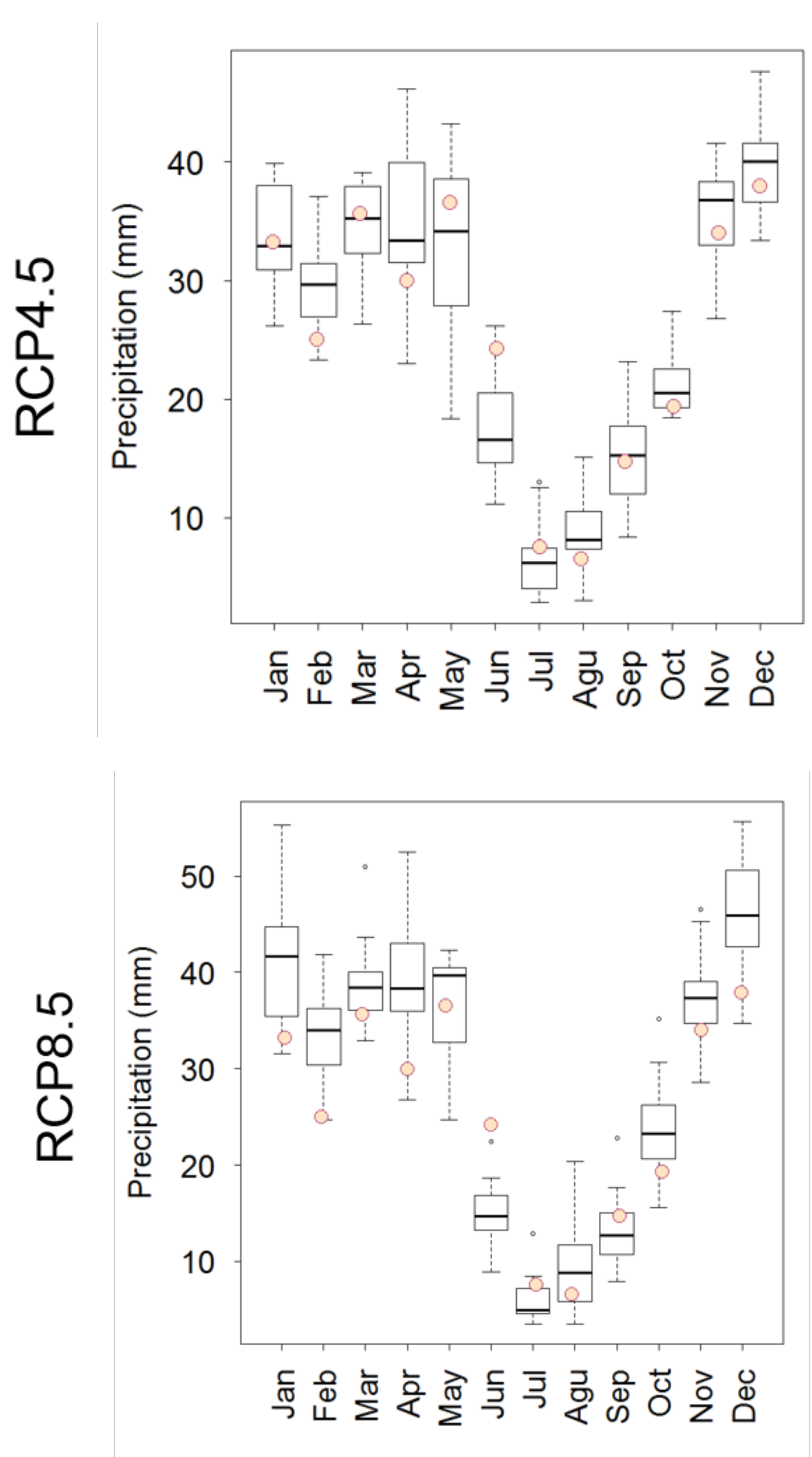
Thirteen monthly climate statistics are required as inputs to WXGN (Table 2) and are calculated directly from daily weather observations (PAST scenario) and statistically downscaled GCM data (RCP4.5 and RCP8.5 scenarios). This results in one set of statistics shown in Table 2 for the PAST scenario, 11 sets (one for each GCM) for the RCP4.5 scenario, and 11 sets (one for each GCM) for the RCP8.5 scenario. For scenarios RCP4.5 and RCP8.5, the collection of these monthly climate statistics across all eleven downscaled GCM outputs represent an empirical density function of climate statistics required as inputs to WXGN. An example of the between-GCM variability in monthly precipitation is shown for scenarios RCP4.5 and RCP8.5 in Figure 3.
For scenarios RCP4.5 and RCP8.5, we then create a realization of the 13 climate statistics required as inputs to WXGN by drawing samples from between the 25th and 75th percentiles of their corresponding empirical density functions. Drawing from between the 25th and 75th percentiles removes potentially extreme variations in monthly climate statistics associated with any individual GCM. Owing to the relatively small number of GCMs available, we used a stratified random sampling technique (Latin Hypercube Sampling; LHS). LHS divides probability space into equal intervals and draws randomly from within each interval. The empirical density function is then inverted to obtain a stratified random parameter sample. LHS ensures that parameters with a relatively low probability of occurrence are sampled, even when using a small number of random samples. Using LHS with 10 strata, we generated 10 realizations of the monthly climate statistics required as input to WXGN for both the RCP4.5 and RCP8.5 scenario groups.
We then input each of these 10 stochastic realizations of monthly climate statistics to WXGN to create 10 stochastic realizations of daily weather for scenario groups RCP4.5 and RCP8.5. For each scenario, we generated 30 years of daily weather. Similarly, we used the monthly climate statistics from the PAST scenario to generate 10 realizations of daily weather for recent past conditions. This results in 100 realizations of 30 years of daily weather data for the RCP4.5 scenario group, 100 realizations of 30 years of daily weather data for the RCP8.5 scenario group, and 10 realizations of 30 years of weather data for the PAST scenario. These daily weather datasets were used as inputs to the Envision-based model of the coupled human-hydrologic system model described below.
3.2. Coupled Socio-Hydrology Systems Model
An integrated socio-hydrologic model that simulates spatially explicit water use based on local water rights is used to evaluate spatiotemporal patterns of water scarcity in the context of the climate scenarios described above. A detailed overview of the biophysical and water rights components of the model, the datasets used to parameterize boundary conditions, calibration to and verification against PAST data, and limitations of the model in the context of those calibration/verification exercises was previously described by [17]. Here we provide a brief overview of the key model components pertinent to this study.
The socio-hydrologic model is developed within the Envision modeling framework, a spatially explicit multi-agent simulation platform for evaluating potential landscape changes arising from interactions between and among complex biophysical and social processes [24]. The model used here employs a slightly revised semi-conceptual Hydrologiska Byråns Vattenbalansavdelning (HBV) model to simulate hydrologic processes. The HBV model is implemented here as a semi-lumped model, operating on spatial elements of Hydrologic Response Units (HRUs) with relatively similar elevations and land cover. At each HRU, the instantaneous temporal change in five water reservoirs (snow, soil moisture, an upper groundwater reservoir, a lower groundwater reservoir, and lake storage) is balanced by incoming precipitation, outgoing evapotranspiration, and outgoing runoff fluxes.
Irrigation activities are simulated based on water rights data provided by the Idaho Department of Water Resources; these water rights are based on the Doctrine of Prior Appropriation [25]. Each record in the water rights dataset is associated with: (1) A priority date on which a water user is entitled to withdrawals from the surface water distribution system, (2) the geographic point of diversion, (3) the maximum diversion rate from the point, and (4) the geographic place of use. Within each time step and for each HRU, the model examines the available water in the stream, the biophysical water demand of the agricultural land within the HRU, and the water rights associated with a place of use coincident with the HRU. Water allocated for irrigation is the minimum of these three quantities. The unsatisfied water is the difference between the amount of water demanded and allocated for each place of use in the model. Detailed descriptions of the calibration and validation processes and the underlying algorithms are described by [17].
As previously stated, the upstream surface water hydrology boundary condition in the Lower Boise River Basin corresponds to the hydrologic output of a system of large reservoirs within the UBRB, a snow-dominated, mountain, largely forest-covered watershed. Although climate change, particularly in the form of shifts in the precipitation phase from snow to rain, is expected to significantly alter hydrologic regimes in the UBRB [2], we do not consider these potential changes in order to reduce the complexity of our analysis. As such, the upstream inflow boundary to our simulation domain (the discharge from the Lucky Peak Reservoir) is set to be the same as a normal year, taking 2012 as an example. While future changes in water rights depend on future real estate transactions, growth in the extent of urban areas, and potential changes in water rights laws, we assume that the attributes of the water rights data remain the same over time. Further, we do not take into account technological changes that may significantly increase water use efficiency in the agricultural sector and lead to lower irrigation water demand and actual water use in the future. Given these assumptions, the impacts of climate change on water availability at the watershed were quantified based on the allocated irrigation amount and the unsatisfied irrigation amount for the years from 2071–2100. Since the weather generator replicates the overall statistics instead of “predicting” inter-annual differences, the comparison between any specific two years within a scenario group is meaningless. As such, we treat the data of each year as an independent realization of the potential outcomes within the large ensemble of data over the thirty years of simulation. Ensemble characteristics and statistics are then compared between the three scenario groups.
4. Datasets
Environmental forcing data used in this study corresponds to the statistically downscaled output from a suite of GCMs that are summarized in Table 1. Each forcing dataset includes daily precipitation, maximum temperature, minimum temperature, specific humidity, solar radiation, and wind speed. These variables, required as input drivers to the socio-hydrologic model, were extracted for the grid point that coincides with the Boise Air Terminal (43.5644° N, 116.2228° W) for the years 2071–2100 to represent the local future climate. Recent past data of the same forcing variables at Boise Air Terminal were obtained from the National Climatic Data Center and National Solar Radiation Database for the period 1981–2014. Other datasets used in the model, including water rights data, Lucky Peak reservoir inflow data, stream discharge data, land use data, and watershed boundaries, were described in detail in [17] and are summarized in Table 3.
5. Results
5.1. Climate Change Analysis
To illustrate the degree to which the use of the stochastic weather generator captures variations in key climate parameters across GCMs, we show the probability density functions (PDFs) of the output of the stochastic weather generator for annual precipitation amount, maximum temperature, and minimum temperature (Figure 4). Overall, the most likely precipitation amount in the RCP8.5 scenario group is larger than that in the RCP4.5 group and PAST group, as shown in the probability density function figure (Figure 4). The average annual precipitation increases by 11% from PAST to RCP4.5 conditions, and by 29% to RCP8.5 conditions. However, a significant overlap between precipitation probability density functions exists in the three scenario groups. For example, it is likely that precipitation in RCP8.5 is smaller than that in RCP4.5 or even the PAST group in some sets of climate realizations.
The PDFs of maximum temperature and minimum annual temperature increase significantly in the future and are much narrower in comparison to the precipitation pattern (Figure 5). The annual mean maximum/minimum temperature is highest in the RCP8.5 scenario group and lowest in the PAST scenario group. The maximum temperatures in the RCP8.5 group and RCP4.5 group are consistently higher than that in the PAST scenario group, by an average of 4.1 °C and 1.7 °C, respectively. The minimum temperatures in RCP8.5 and RCP4.5 groups are consistently larger than that in the PAST scenario by an average of 5.6 °C and 3.2 °C, respectively. The average daily temperature increases by 4.9 °C in the RCP8.5 scenario group, and by 2.5 °C in the RCP4.5 scenario group. Temperature increase in the Treasure Valley is at the higher end of the IPCC CIMP5 projected global trend which, in general, projects a temperature increase of 1.1 °C to 2.6 °C for RCP4.5, and an increase of 2.6 °C to 4.8 °C for RCP8.5 by the end of the 21st century [26].
5.2. Irrigation Water Analysis
The simulation results from a total of 210 runs of the integrated socio-hydrologic model indicate, unsurprisingly, that more irrigation water is needed to fulfill the crop water demand in the future. The average annual allocated irrigation water is highest in the RCP8.5 scenario group (Figure 6). The average annual allocated irrigation water in both RCP4.5 (1.0 × 10⁹ m3) and RCP8.5 (1.1 × 10⁹ m3) scenario groups is higher than the PAST scenario (8.3 × 10⁸ m3), an increase of 20.5% and 32.5%, respectively. However, the ensembles between the three scenarios overlap with one another due to the extremes captured by realizations of the weather generator. This overlap indicates extreme water use scenarios that deviate significantly from the average future projections. As such, although examining the mean/median values from a large ensemble of the analysis is useful for understanding the central tendencies of potential future agricultural water demands in the region, the entirety of the ensemble allows a more sophisticated interpretation of potential future outcomes, particularly those that could be low probability events but of significant consequences.
Similar to the allocated amount, the average annual unsatisfied irrigation water is also highest for the RCP8.5 scenario group (Figure 7). The average annual unsatisfied irrigation water in both RCP4.5 and RCP8.5 scenario groups are higher than the PAST scenario group. Similar with allocated irrigation water, there is also overlap in unsatisfied irrigation between all scenarios. The mean value of the unsatisfied water increases from about 2.1 × 10⁷ m3 in the PAST scenario group to about 3.3 × 10⁷ m3 in the RCP4.5 scenario group and 5.2 × 10⁷ m3 in the RCP8.5 scenario group, an increase of 57.1% and 147.6%, respectively. The results underscore the value of using ensembles of model simulations to assess potential future outcomes, as a few realizations were associated with extreme values of unsatisfied irrigation that are not reflected in the central tendencies of the PDFs.
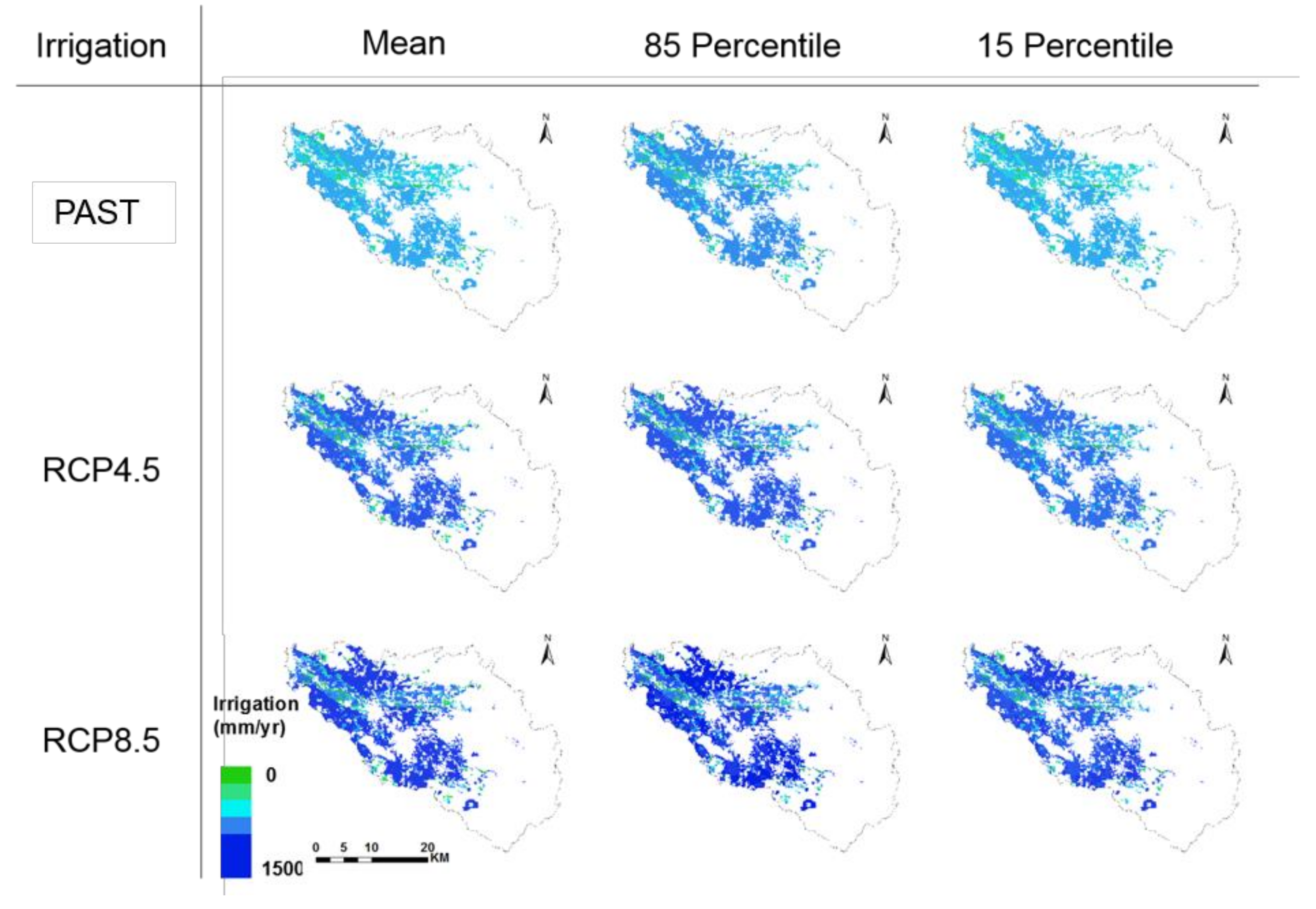
The ensemble simulation also allows us to assess spatial locations within the domain most likely to be associated with unsatisfied water demand under future climates and, by comparing this to geospatial data characterizing biophysical and social constraints on hydrology in the region, to draw inference about key characteristics of the landscape associated with water shortages (Figure 8 and Figure 9). The model-simulated allocation rate indicates that the Southwest part of the study domain receives the most allocated water, while the corridor immediately abutting the downstream portions of the Boise River receives relatively less allocated water. Conversely, the unsatisfied irrigation water value is largest along the downstream Boise River.
However, there is also a significant amount of water scarcity in the Southwest part of the domain (the Wilder Irrigation District approximate to Lake Lowell). Throughout the domain, where there is water allocated to irrigation, there is a significant increase in both the water use and water scarcity relative to PAST conditions in the RCP 4.5 and RCP 8.5 conditions. Looking more specifically at the Southwest part (Wilder Irrigation District), the mean allocated irrigation rate increases from 737 mm/y to 909 mm/yr to 996 mm/yr from the PAST to the RCP4.5, and then to the RCP8.5 scenario groups, an increase of 23% and 35%, respectively. Although the area is classified as senior in water rights (water rights in the region were claimed between 1864 to 1927), the mean unsatisfied irrigation rate increases from 13 mm/y to 19 mm/y to 31 mm/y from the PAST to the RCP 4.5, and then to the RCP 8.5 scenario groups, an increase of 46% and 138% respectively. Using ensemble mean values avoids the large discrepancies from individual simulations. For example, the allocated irrigation rate at the 85th percentile varies from 789 mm/y in the PAST to 948 mm/y in the RCP4.5 to 1041 mm/y in the RCP8.5 groups, and the unsatisfied irrigation rate at the 85th percentile varies from 20 mm/y in the PAST to 27 mm/yr in the RCP4.5 to 42 mm/yr in the RCP8.5 groups.
6. Discussion
6.1. Adopting Stochastic Weather Generators with GCM Output May Avoid the Deficiencies Employing Individual Method
The use of multiple GCM projections in combination with the stochastic weather generator to generate ensembles of future climate realizations offers some key advantages in assessing the potential future ramifications for coupled socio-hydrologic systems. The results are broadly consistent with the GCM output but also account for variability in climatic conditions as captured by a variety of GCMs while providing insights into local climatic perturbations.
First, the method allows for an unlimited number of future daily climate data with monthly statistics that are derived from multiple GCMs. In this way, the method avoids the deficiencies of using a single GCM or a simple mean of multiple GCMs that may lead to biased future projections and also avoids the deficiencies of a limited number of GCMs that cannot provide enough reliable daily climate data for hydrologic models.
Second, stochastic weather generators (like WXGN) are a relatively computationally inexpensive method for generating the daily climate variables needed by a diverse array of hydrologic and ecological models. They are also relatively easy to use and parameterize, making them amenable to a variety of different climate change assessment applications and techniques. The resulting ensemble of outputs generated with the corresponding ensemble of climate realizations used as inputs allows for a more sophisticated analysis of the potential future impacts of climate change, both in terms of the central tendencies of change and potentially low-risk, high-consequence outcomes.
It should be added that the proposed method is not appropriate for all circumstances. The method we develop and apply here is most suitable for hydrologic and ecologic models that need numerous sets of long-term daily climate inputs. For example, in our case study, we need daily hydrologic simulations to allow for real-time water rights allocations. The method may not be necessary for all conceptual modes or lump-sum models that only require rough water balance estimations. Although the application of the stochastic weather generator to create ensembles of climate inputs to a socio-hydrologic model is a methodologically straightforward process, simulating an ensemble of climate realizations still requires a relatively large amount of computational time. This is particularly true for spatially distributed hydrologic models. There is, therefore, a need to balance larger ensembles against higher spatial resolutions when a spatially distributed model is being used.
6.2. The Effects of Climate Change on Regional Scale Hydrology and Irrigation
Both temperature and precipitation are important climate variables that affect regional hydrology and irrigation demand. Temperature directly influences potential evapotranspiration and crop water demand (Figure 10, Figure 11). Under the same upstream inflow conditions, the allocated and unsatisfied irrigation water has a clear monotonic relationship with temperature across the scenario groups. There is an increase in the allocated irrigation amount with the increase of the maximum temperature and the minimum temperature. Although there is significant overlap between scenario groups, the overall trend of an increasing irrigation water demand and scarcity from PAST conditions to RCP4.5 and RCP8.5 is evident.
The influence of precipitation on allocated and unsatisfied water is not as clear as that of temperature (Figure 12). In the Treasure Valley, over half of the precipitation happens in the non-irrigation season, and most of the irrigation water relies on diversion from streams and reservoirs. As such, precipitation change in the immediate region of the Treasure Valley is not as important as temperature change with regard to water demand and use. Instead, precipitation in the upper Boise River Basin that provides snowpack for irrigation water will exert a more significant influence on downstream water demand.
6.3. Limitations
This study has limitations that readers should keep in mind while interpreting the results. In order to illustrate the influence of climate change as an important factor on the water availability of the region, we made choices with significant implications on socio-biophysical changes in the future. We do not consider population and land use change, which are both important changing factors for future water use projections. We also assume that the recharge into the watershed boundary keeps constant between years; however, research has shown that recharge from Upper Boise Watershed to the study area will change under future climate change scenarios [2]. In addition, we also assume that water rights will remain the same in the future. However, changes are expected due to water right transitions with real estate transactions, land use changes, and potential changes in water rights laws. However, categorizing future dynamic water rights change is beyond the scope of the research, and the method will be applicable with newly updated water rights data once it is available. Technological changes and irrigation patterns may change in the future, e.g., shifts of flood irrigation to micro-irrigation systems (trickle or drip) that may significantly increase water use efficiency in the agricultural sector and lead to a lower irrigation water demand and actual water use in the future. Sprinkler and flood irrigation system are still dominating in the U.S. [27], but micro-irrigation systems are getting more popular, which will change the water use efficiency greatly. Uncertainties may also arise during the integration of these complex socio-biophysical processes since many of these processes are interrelated and non-linear. Nonetheless, this work aims to illustrate the use of the new climate data generation method, and it is a vital step towards moving into a more comprehensive model. While the quantity of the water scarcity projections may change after considering more factors, the quality or trajectories of the projections will stand due to the anticipated effects of climate change. The information provided in this study can help stakeholders think about future water use strategies to mitigate climate change.
7. Conclusions
This study develops an ensemble approach for creating daily climate realizations combining a stochastic weather generator and downscaled General Circulation Model (GCM) projections. The generated ensemble of climate data is then used to drive an integrated socio-hydrologic model using the Envision scenario-based modeling framework. In this way, the model captures both spatially explicit irrigation activities constrained by local water rights, and future changes in climate and their impact on atmospheric water demand in the region. We tested this model in a rapidly growing region of Idaho, USA. Results show that, on average, precipitation amount increases slightly, and temperature increases significantly in future climate scenarios. Temperature increases are particularly pronounced in the RCP8.5 scenarios. The increase of temperature has a direct influence on the increase of the allocated and unsatisfied irrigation amount, while the impacts of slightly increased mean annual precipitation (but increased interannual variability in mean annual precipitation) on water use are less obvious and more uncertain. The model also predicts spatial patterns in water allocation and scarcity and the ensemble approach allows us to identify regions within the study area that will be more prone to insufficient water supply in the future. Although the developed model is associated with some key simplifications that limit, for instance, the ability to draw inferences about future groundwater-surface water interactions, the approach presented here could be applied to more sophisticated modeling frameworks to elicit broader conclusions about system behavior. Moreover, the framework presented here is portable to other geographic settings where legal frameworks dictate the timing, amount, and priorities of water use.
Author Contributions
Conceptualization, A.N.F. and B.H.; Methodology, B.H. and A.N.F.; Formal Analysis, B.H.; Investigation, B.H.; Resources, A.N.F. and S.G.B.; Data Curation, B.H. and A.N.F.; Writing-Original Draft Preparation, B.H.; Writing-Review & Editing, B.H., A.N.F., and S.G.B.; Supervision, A.N.F. and S.G.B.; Project Administration, A.N.F., and S.G.B.; Funding Acquisition, A.N.F., and S.G.B..
Funding
This research was funded by National Science Foundation (NSF) Idaho Established Program to Stimulate Competitive Research (EPSCoR) under award number IIA-1301792, NSF CAREER Award EAR-1352631, and a Ball State University new faculty start-up fund under award number 120198.
Acknowledgments
We would like to thank Javier M. Osorio Leyton from Texas A&M for the help with WXGN, and Katherine Hegewisch from University of Idaho for the MACA data collection. We also thank the Envision team from Oregon State University for the help with the hydrologic model construction and debugging. Data associated with this manuscript has been permanently archived and made public with doi:10.18122/B20133.
Conflicts of Interest
The authors declare no conflict of interest.
Appendix A. Boxplot of Monthly Climate Statistics (12 Variables) of 11 Selected GCMs. The Circles Indicate the PAST Monthly Average
 |
 |
References
- Klos, P.Z.; Link, T.E.; Abatzoglou, J.T. Extent of the rain-snow transition zone in the western US under historic and projected climate. Geophys. Res. Lett. 2014, 41, 4560–4568. [Google Scholar] [CrossRef]
- Steimke, A.L.; Han, B.; Brandt, J.S.; Flores, A.N. Climate Change and Curtailment: Evaluating Water Management Practices in the Context of Changing Runoff Regimes in a Snowmelt-Dominated Basin. Water 2018, 10, 1490. [Google Scholar] [CrossRef]
- Vano, J.A.; Nijssen, B.; Lettenmaier, D.P. Seasonal hydrologic responses to climate change in the Pacific Northwest. Water Resour. Res. 2015, 51, 1959–1976. [Google Scholar] [CrossRef]
- Giorgi, F.; Jones, C.; Asrar, G.R. Addressing climate information needs at the regional level: The CORDEX framework. World Meteorol. Org. (WMO) Bull. 2009, 58, 175. [Google Scholar]
- Hawkins, E.; Sutton, R.; Hawkins, E.; Sutton, R. The Potential to Narrow Uncertainty in Regional Climate Predictions. Bull. Am. Meteorol. Soc. 2009, 90, 1095–1108. [Google Scholar] [CrossRef]
- Abatzoglou, J.T. Development of gridded surface meteorological data for ecological applications and modelling. Int. J. Climatol. 2013, 33, 121–131. [Google Scholar] [CrossRef]
- Abatzoglou, J.T.; Brown, T.J. A comparison of statistical downscaling methods suited for wildfire applications. Int. J. Climatol. 2012, 32, 772–780. [Google Scholar] [CrossRef]
- Dosio, A.; Paruolo, P. Bias correction of the ENSEMBLES high-resolution climate change projections for use by impact models: Evaluation on the present climate. J. Geophys. Res. Atmos. 2011, 116, D16. [Google Scholar] [CrossRef]
- Chen, J.; François, P.B.; Leconte, R. A daily stochastic weather generator for preserving low-frequency of climate variability. J. Hydrol. 2010, 388, 480–490. [Google Scholar] [CrossRef]
- Richardson, C.W. Stochastic simulation of daily precipitation, temperature, and solar radiation. Water Resour. Res. 1981, 17, 182–190. [Google Scholar] [CrossRef]
- Richardson, C.W.; Wright, D.A. WGEN: A Model for Generating Daily Weather Variables; US Department of Agriculture, Agricultural Research Service: Washington, DC, USA, 1984. [Google Scholar]
- Semenov, M.A.; Barrow, E.M. Use of a Stochastic Weather Generator in the Development of Climate Change Scenarios. Clim. Chang. 1997, 35, 397–414. [Google Scholar] [CrossRef]
- Wilks, D.S. Use of stochastic weathergenerators for precipitation downscaling. WIREs Clim. Chang. 2010, 1, 898–907. [Google Scholar] [CrossRef]
- Xu, C.Y. From GCMs to river flow: A review of downscaling methods and hydrologic modelling approaches. Prog. Phys. Geogr. 1999, 23, 229–249. [Google Scholar] [CrossRef]
- Petrich, C.R. Treasure Valley Hydrologic Project Executive Summary; Idaho Water Resources Research Institute: Boise, ID, USA, 2004. [Google Scholar]
- Urban, S.M.; Petrich, C.R. Water Budget for the Treasure Valley Aquifer System; Treasure Valley Hydrologic Project Research Report; Idaho Department of Water Resources: Boise, ID, USA, 1996. [Google Scholar]
- Han, B.; Benner, S.G.; Bolte, J.P.; Vache, K.B.; Flores, A.N. Coupling biophysical processes and water rights to simulate spatially distributed water use in an intensively managed hydrologic system. Hydrol. Earth Syst. Sci. 2017, 21, 3671–3685. [Google Scholar] [CrossRef]
- Bouzaher, A.; Shogren, J.F.; Holtkamp, D.; Gassman, P.W.; Archer, D.; Lakshminarayan, P.G.; Carriquiry, A.L.; Reese, R. Agricultural Policies and Soil Degradation in Western Canada: An Agro-Ecological Economic Assessment, Report 2: The Environmental Modeling System; Center for Agricultural and Rural Development (CARD) at Iowa State University: Ames, IA, USA, 1994. [Google Scholar]
- Forsythe, N.; Fowler, H.J.; Blenkinsop, S.; Burton, A.; Kilsby, C.G.; Archer, D.R.; Harpham, C.; Hashmi, M.Z. Application of a stochastic weather generator to assess climate change impacts in a semi-arid climate: The Upper Indus Basin. J. Hydrol. 2014, 517, 1019–1034. [Google Scholar] [CrossRef]
- Hayhoe, H.N.; Stewart, D.W. Evaluation of CLIGEN and WXGEN weather data generators under Canadian conditions. Can. Water Resour. J. 1996, 21, 53–67. [Google Scholar] [CrossRef]
- Kilsby, C.G.; Jones, P.D.; Burton, A.; Ford, A.C.; Fowler, H.J.; Harpham, C.; James, P.; Smith, A.; Wilby, R.L. A daily weather generator for use in climate change studies. Environ. Model. Softw. 2007, 22, 1705–1719. [Google Scholar] [CrossRef]
- Racsko, P.; Szeidl, L.; Semenov, M. A serial approach to local stochastic weather models. Ecol. Model. 1991, 57, 27–41. [Google Scholar] [CrossRef]
- Qian, B.; Gameda, S.; Hayhoe, H.; De Jong, R.; Bootsma, A. Comparison of LARS-WG and AAFC-WG stochastic weather generators for diverse Canadian climates. Clim. Res. 2004, 26, 175–191. [Google Scholar] [CrossRef]
- Bolte, J.P.; Hulse, D.W.; Gregory, S.V.; Smith, C. Modeling biocomplexity–actors, landscapes and alternative futures. Environ. Model. Softw. 2006, 22, 570–579. [Google Scholar] [CrossRef]
- Tarlock, A.D. Prior appropriation: Rule, principle, or rhetoric. N.D.L. Rev. 2000, 76, 881. [Google Scholar]
- Stocker, T.F. Climate Change 2013: The Physical Science Basis: Working Group I Contribution to the Fifth Assessment Report of the Intergovernmental Panel on Climate Change; Cambridge University Press: Cambridge, UK, 2014. [Google Scholar]
- USGS. Irrigation Water Use. 2015. Available online: https://water.usgs.gov/watuse/wuir.html (accessed on 23 January 2019).
Figure 1.
Study area: Treasure Valley.

Figure 2.
The workflow for creating forcing ensembles.

Figure 3.
A boxplot of monthly climate variables over 11 GCMs, using only precipitation as an example. The boxplot of the other 12 variables is included in the Appendix A. The circles indicate the recent past (PAST) monthly precipitation. The large variance indicates that an ensemble of climate realizations is necessary to capture the variations of future climate change.

Figure 4.
The annual precipitation used to drive the hydrologic model.

Figure 5.
The annual maximum (Tmax) and minimum (Tmin) temperatures used to drive the hydrologic model.
Figure 5.
The annual maximum (Tmax) and minimum (Tmin) temperatures used to drive the hydrologic model.


Figure 6.
The annual amount of allocated irrigation water under 3 different scenarios.

Figure 7.
The annual amount of unsatisfied irrigation water under 3 different scenarios.

Figure 8.
The annual amount of allocated irrigation water under 3 different scenario groups (spatial maps show the mean, 85th, and 15 percent range for each scenario group).
Figure 8.
The annual amount of allocated irrigation water under 3 different scenario groups (spatial maps show the mean, 85th, and 15 percent range for each scenario group).

Figure 9.
The annual amount of unsatisfied irrigation water under 3 different scenario groups (spatial maps show the mean, 85th, and 15 percent range for each scenario group).
Figure 9.
The annual amount of unsatisfied irrigation water under 3 different scenario groups (spatial maps show the mean, 85th, and 15 percent range for each scenario group).

Figure 10.
The scatterplot of the allocation irrigation amount and the unsatisfied irrigation amount with maximum and minimum temperature under three scenario groups. The solid dots indicate the mean values of each scenario group.
Figure 10.
The scatterplot of the allocation irrigation amount and the unsatisfied irrigation amount with maximum and minimum temperature under three scenario groups. The solid dots indicate the mean values of each scenario group.

Figure 11.
The annual level of the evapotranspiration rate under 3 different scenario groups.

Figure 12.
The scatterplot of the allocation irrigation amount and the unsatisfied irrigation amount with precipitation under three scenario groups. The solid dots indicate the mean values of each scenario group.
Figure 12.
The scatterplot of the allocation irrigation amount and the unsatisfied irrigation amount with precipitation under three scenario groups. The solid dots indicate the mean values of each scenario group.


Table 1.
The CMIP5 models used in this study for downscaled climate data and the model development centers.
Table 1.
The CMIP5 models used in this study for downscaled climate data and the model development centers.
| Model | Development Center |
|---|---|
| BNU-ESM | College of Global Change and Earth System Science, Beijing Normal University, China |
| CanESM2 | Canadian Center for Climate Modeling and Analysis |
| CNRM-CM5 | National Center of Meteorological Research, France |
| CSIRO-Mk3-6-0 | Commonwealth Scientific and Industrial Research Organization/Queensland Climate Change Center of Excellence, Australia |
| GFDL-ESM2G | NOAA Geophysical Fluid Dynamics Laboratory, USA |
| GFDL-ESM2M | NOAA Geophysical Fluid Dynamics Laboratory, USA |
| IPSL-CM5A-LR | Institut Pierre Smon Laplace, France |
| IPSL-CM5A-MR | Institut Pierre Smon Laplace, France |
| IPSL-CM5B-LR | Institut Pierre Smon Laplace, France |
| MIROC5 | Atmosphere and Ocean Research Institute (The University of Tokyo), National Institute of Environmental Studies, and Japan Agency for Marine-Earth Science and Technology |
| MRI-CGCM3 | Meteorological Research Institute, Japan |
Table 2.
13 climate variables summarized from General Circulation Models (GCMs) for WXGN use to generate the ensemble of daily climate realizations.
Table 2.
13 climate variables summarized from General Circulation Models (GCMs) for WXGN use to generate the ensemble of daily climate realizations.
| Variable | Description |
|---|---|
| PRECIP | Average monthly precipitation |
| TMAX | Average monthly maximum air temperature |
| TMIN | Average monthly minimum air temperature |
| PWD | Monthly probability of wet day after dry day |
| PWW | Monthly probability of wet day after wet day |
| DAYP | Average number days of rain per month days |
| RAD | Average monthly solar radiation |
| SDMX | Monthly average standard deviation of daily maximum temperature |
| SDMM | Monthly average standard deviation of daily minimum temperature |
| SDRF | Monthly standard deviation of daily precipitation |
| SKRF | Monthly skew coefficient for daily precipitation |
| RH | Monthly average relative humidity (fraction) |
| WS | Average monthly wind speed |
Table 3.
Datasets used and the source link in the study.
| Input Data | Data Source | Year | Use in Model | Link |
|---|---|---|---|---|
| Streams | NHDPlus | 2012 | Build stream network and flow routing | http://www.horizon-systems.com/nhdplus/NHDPlusV2_17.php |
| Land use/land cover | National Landcover dataset (NLCD) | 2011 | Evaportranspirtaion | http://www.mrlc.gov/nlcd2011.php |
| Water Rights | Idaho Department of Water Resources (IDWR) | 2010 | Irrigation (Watermaster) | http://www.idwr.idaho.gov/ftp/gisdata/Spatial/WaterRights |
| Major climate variables | National Climatic Data Center (NCDC) | 1981–2014 | Climate input | http://www7.ncdc.noaa.gov/CDO/cdodata.cmd |
| Solar radiation | National Renewable Energy Laboratory (NREL) | 1981–2010 | Climate input | http://rredc.nrel.gov/solar/old_data/nsrdb/ |
| Reservoir Inflow | Hydromet Pacific Northwest Region | 2012 | Inflow boundary | http://www.usbr.gov/pn/hydromet/arcread.html |
© 2019 by the authors. Licensee MDPI, Basel, Switzerland. This article is an open access article distributed under the terms and conditions of the Creative Commons Attribution (CC BY) license (http://creativecommons.org/licenses/by/4.0/).
Share and Cite
MDPI and ACS Style
Han, B.; Benner, S.G.; Flores, A.N. Including Variability across Climate Change Projections in Assessing Impacts on Water Resources in an Intensively Managed Landscape. Water 2019, 11, 286. https://doi.org/10.3390/w11020286
AMA Style
Han B, Benner SG, Flores AN. Including Variability across Climate Change Projections in Assessing Impacts on Water Resources in an Intensively Managed Landscape. Water. 2019; 11(2):286. https://doi.org/10.3390/w11020286
Chicago/Turabian StyleHan, Bangshuai, Shawn G. Benner, and Alejandro N. Flores. 2019. "Including Variability across Climate Change Projections in Assessing Impacts on Water Resources in an Intensively Managed Landscape" Water 11, no. 2: 286. https://doi.org/10.3390/w11020286
Note that from the first issue of 2016, this journal uses article numbers instead of page numbers. See further details here.