Optimizing the Formation of DMAs in a Water Distribution Network through Advanced Modelling


1
Department of Civil Engineering, University of Thessaly, 38334 Volos, Greece
2
Department of Electrical and Computer Engineering, University of Thessaly, 38221 Volos, Greece, [email protected]
*
Author to whom correspondence should be addressed.
Water 2019, 11(2), 278; https://doi.org/10.3390/w11020278
Submission received: 25 October 2018
/
Revised: 18 December 2018
/
Accepted: 31 January 2019
/
Published: 6 February 2019
(This article belongs to the Special Issue Insights on the Water–Energy–Food Nexus)
Abstract
:Water pressure management in a water distribution network (WDN) is a key component applied to achieve desirable water quality as well as a trouble-free operation of the network. This paper presents a hybrid, two-stage approach, to provide optimal separation of a WDN into District Metered Areas (DMAs), improving both water age and pressure. The first stage aims to divide the WDN into smaller areas via the Geometric Partitioning method, which is based on Recursive Coordinate Bisection (RCB). Subsequently, the Student’s t-mixture model (SMM) is applied to each area, providing an optimal placement of isolation valves and separating the network in DMAs. The model is evaluated on a realistic network generated through Watergems and is compared against one variation of it implemented, including the Gaussian Mixture Model (GMM) as well as the Genetic Algorithm (GA) approach, obtaining impressive performance. The implementation of both stages was deployed in a MATLAB environment through the Epanet toolkit. The proposed system is very promising, especially for large size WDNs due to the decreased running time and noteworthy reduction of pressure and water age.
1. Introduction
The need to efficiently manage big and complex water distribution networks in most metropolitan areas is the driving force that makes water utility managers divide these systems into sub-regions called District Metered Areas (DMAs) [1,2,3,4,5]. Their boundaries, inlets and outlets (entrance and exit nodes) are being formed using different types of valves and flow meters, in order to improve pressure management and assist the effective supervision of the networks for leakages. Traditionally, the design of DMAs was based on trial-and-error approaches, being quite difficult to apply to large networks. Moreover, the results were not optimal. Lately, new techniques based on graph theory [6] have been proposed by many researchers. In addition, metaheuristic methods inspired by nature are also very popular. One of the most well-known methods in the field is the Genetic Algorithm, inspired by Charles Darwin’s theory of natural evolution. This method has been employed by many researchers over the last decades [7]. Other evolutionary methods such as Simulation Annealing (SA), Ant colony [8], and Shuffled Complex Evolution (SCE) method have also been used [9].
However, due to the large number of simulations required in most heuristic methods, it is very important for researchers to find the least time-consuming method for WDN analysis. A very popular way is to combine two or more methods and create multiple phase strategies [10,11,12]. Another approach that has been proposed is the one introduced by Diao and Zhou [13], where a boundary generator is created based on artificial intelligence to determine the DMAs. Perelman and Allen [10] compared different methodologies, and concluded that community structures play a vital role in the sectorization of the network.
In this paper, a two-phase approach was used, implementing the example of ‘divide and conquer’ to simplify the DMAs’ formation process and reduce the computational time. By dividing the water network into DMAs, installing properly selected gate valves and flow meters along the network, the detection of the WDN for leakage is easier, water losses are reduced, and the quality of water is improved. The main idea is to combine two different phases, a phase of dividing and a phase of clustering. Generally, such a two-step approach allows simplifying the water network partitioning, as, once the first division is identified, it becomes the starting point of the subsequent clustering phase. More precisely, the first one, based on Recursive Coordinate Bisdection, which is actually a geometric process, creates a first division of the network into equal sized zones. The second one, which is based on probabilistic methods, is applied on every previously created subregion, in a parallel manner, to optimize the average pressure and the water age across the entire network, by creating clusters in every subregion and finalize the DMAs’ formation. For the second step, three algorithms are compared, namely Gaussian Mixture Modelling, Mixtures of Student’s t-distribution and Genetic Algorithm, showcasing the one that gives the best result to our task. The evaluation of the proposed approach is performed employing the Net 22 network, included in the Watergems tool library, and the realistic network of Aiani, a suburb of Kozani city in Greece.
2. Proposed Methods
2.1. Recursive Coordinate Bisection-RCB
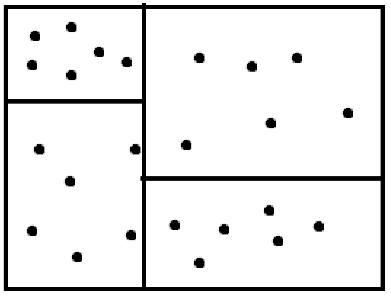
Geometric partitioning is a very useful method for quick division of a list of coordinates into approximately equal-sized regions of spatially close elements. The most common algorithm for geometric partitioning involves the recursive generation of a series of cutting planes, which bisect the mesh. The Geometric Partitioning algorithm is based on Recursive Coordinate Bisection (RCB) [14,15], which is attractive as a dynamic load-balancing algorithm. The creation of each subregion depends only on the actual place every node is and not on other parameters like the elevation or the demand. It is actually an easy way to create equal size zones, especially in large networks, where the number of nodes is huge. The network is divided into two roughly equal sized sub-regions by an orthogonal cutting plane to the most elongated axe and then the separation continues recursively in every sub-area until the regions that created reach the intended number (Figure 1). Each pair of planes is orthogonal to the previous one. It is obvious, that if we want, for example, to divide the object into sixteen subdomains, we have to apply the algorithm four times to the dual. Also, the subdomains have a few isolated outlying vertices and no connectivity information enters the RCB. To this point, we should notice that RCB does not create DMAs and no pipe is closing. It divides the network into subzones, to help the second algorithm run in parallel manner for every area and in that way computational time is reduced dramatically.
2.2. Gaussian Mixture Model
Gaussian Mixture Modelling (GMM) is a probabilistic method to represent normally distributed subpopulations within an overall population. It has been commonly used for feature extraction from speech data [16] image segmentation [17,18], biometric systems such as vocal-track related spectral features in a speaker recognition system [19], weather observation in geoscience [20], etc. GMM can be viewed as a mixture of heterogenous populations, whose underlying mean follows a Gaussian distribution. Mathematically, Gaussian mixture models can be considered as parametric probability density functions, which can be represented as a weighted sum of all densities of Gaussian components.
Due to the fact that the problem of water distribution network optimization may be regarded as a clustering problem, the goal is to assign the nodes of each previously generated sub-area to k clusters, with k given [21,22]. Let each node be represented by a variable xn, with n = 1, …, N being the number of nodes in each partition of the Geometric Partitioning algorithm, whose value is equal to the objective function’s value for the node n. Assuming that the independently distributed random variables x are a realization of a Gaussian mixture model (GMM) [23,24], the probability of a single node is denoted by:
where π denotes the probability of the n-th node to belong to the j-th cluster and is constrained to be positive, 0 < < 1, and . Additionally, is a Gaussian distribution with μk denoting the Gaussian kernel mean vector and Σk representing the Gaussian kernel covariance matrices.
To perform the formula inference, we exploit MAP (maximum a posteriori probability) estimation through EM (Expectation-Maximization) algorithm [25]. Thus, the calculation of the parameters πk, μk and Σk is carried out through the GMM-EM algorithm, which is a repetitive algorithm and a powerful method for finding solutions concerning models with hidden variables [23]. The algorithm consists of two steps—the E-step and the M-step—continuously performed until the final convergence. The algorithm begins with a random estimate of the parameters’ initial values. The equations originated from the E-step and M-step of the algorithm are:
,
,
2.3. Mixtures of Student’s t-Distributions
The Student’s t-distribution [26], which is a heavy-tailed alternative of Gaussian probability distribution, is determined by its degrees of freedom, namely the number of independent observations in the dataset.
In the same manner as in Section 2.2 it is assumed that a K-cluster mixture of t-distributions is given by:
with denoting a representation of every node in each partition of the Geometric Partitioning algorithm, μk being the Gaussian kernel mean vector, Σk representing the Gaussian kernel covariance matrices and v ∈ [0, ∞) being the degrees of freedom. Moreover, assuming a d-dimensional random variable x that follows a multivariate t-distribution with mean μ, positive definite, symmetric and real dxd covariance matrix Σ and v ∈ [0, ∞) degrees of freedom has a density expressed by [27]:
where δ(x,μ;Σ) = (x − μ)T Σ−1(x − μ) is the Mahalanobis squared distance and is the Gamma function.
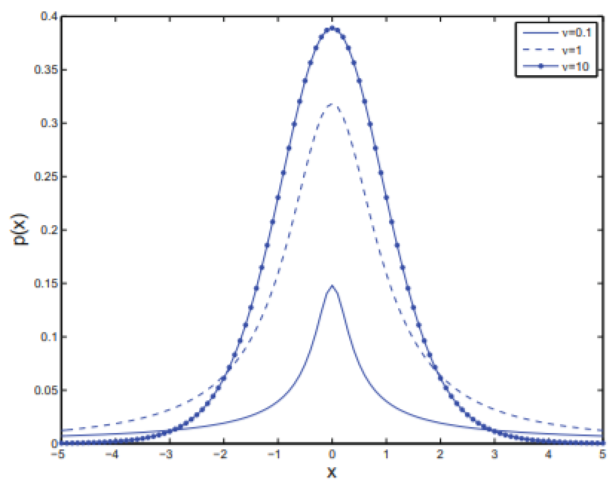
As is shown in Figure 2 for x > ∞ 1, the Student’s t-distribution tends to a Gaussian distribution with covariance Σ. Also, if ν > 1, μ is the mean of X and if ν > 2, ν(ν − 2)−1, Σ is the covariance matrix of X.
A Student’s t-distribution mixture model (SMM) may also be trained using the EM algorithm. Thus, through E-step, the posterior probability of the datum x belongs to the k-th cluster of the mixture as well as the expectation of the weights for each node are computed:
The update equations of the mixture model parameters are given by:
The corresponding degrees of freedom for the k-th cluster, at time step t + 1, are calculated through the following equation:
where ψ(.) is the digamma function.
2.4. Genetic Algorithm
Genetic Algorithm is a method based on natural selection. The general idea of this algorithm is to create an optimal solution relying on bio-inspired operators such as mutation, crossover and selection. In this case, we use the Genetic Algorithm tool of Matlab, working with the following objective function [28]:
where, i represents each node of the network, Di,t is the demand of node I for each time step t (lt/s), Pi,t is the pressure of node I for each time step t (kPa), Pmin is the minimum defined operating pressure (kPa), is the weight of the demand of each node multiplied by the pressure variation of each node. Also, minimum required nodal pressure is defined at 200 kPa for Greek legislation and is followed by all water utilities.
2.5. Forming of the Objective Functions
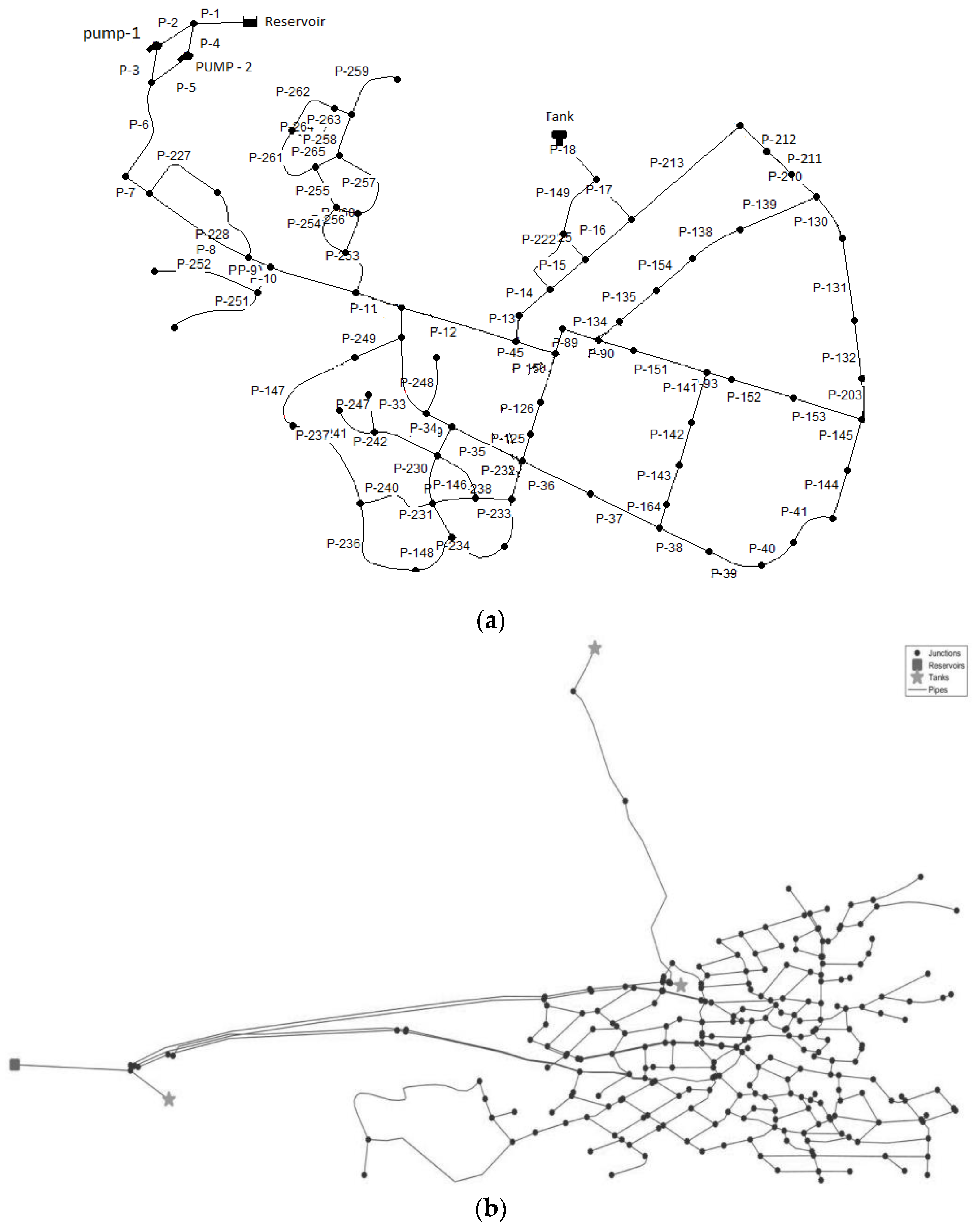
The proposed algorithm was applied to Net 22 (Figure 3a), which is included as an example in the Watergems program (lesson 6). It consists of 100 pipes, one tank, one reservoir and two pumps (boosters) (Figure 3a). Then, a real network of Aiani (Figure 3b) was used. Aiani is a suburb of Kozani city located in the region of Western Macedonia, Greece, covering an area of 152.9 square kilometers. It consists of 329 pipes with a total length of 28,846 m, 140 valves and two tanks. The altitude of the area ranges from 432 m up to 547 m with an average of 460 m. Due to the altitude difference in the area and the gravity effect, water pressure and water quality are significantly affected. After applying the algorithm to each partition created through the Geometric Partitioning, k clusters are created within each region. The objective function for each node I is denoted by the following equation:
where Dit is the demand of node I at each time step t (lt/s) and Pit represents the pressure of node I at each time step t (kPa). The number k of the clusters must be set in a way that it optimizes the fitness function. Moreover, the influence of the algorithm on the water age of the network was examined using the following objective function:
The goal was to minimize the product P × D and the water age, while maintaining the lowest level of pressure (200 kPa) in any node (this limitation is being enforced by the national legislation), and to minimize the total water age. Clusters from each partition having the highest mean average (μk) were selected, and the isolation valves were placed there. The limitations of the model are the following: a) The ending nodes are excluded and cannot be selected; while b) nodesith negative pressures or pressures below 200 kPa (29 psi) are rejected. The algorithms were implemented within a Matlab environment with k = 4 number of sub-regions, and the total product P × D is noted for a 24-h time period. The number k of sub-regions was chosen after evaluation with respect to different number of k, as shown in Table 1, selecting the value that provides the maximum minimization of the objective functions for both networks (row with bold).
3. Results
3.1. Applying the Recursive Coordinate Bisection Approach
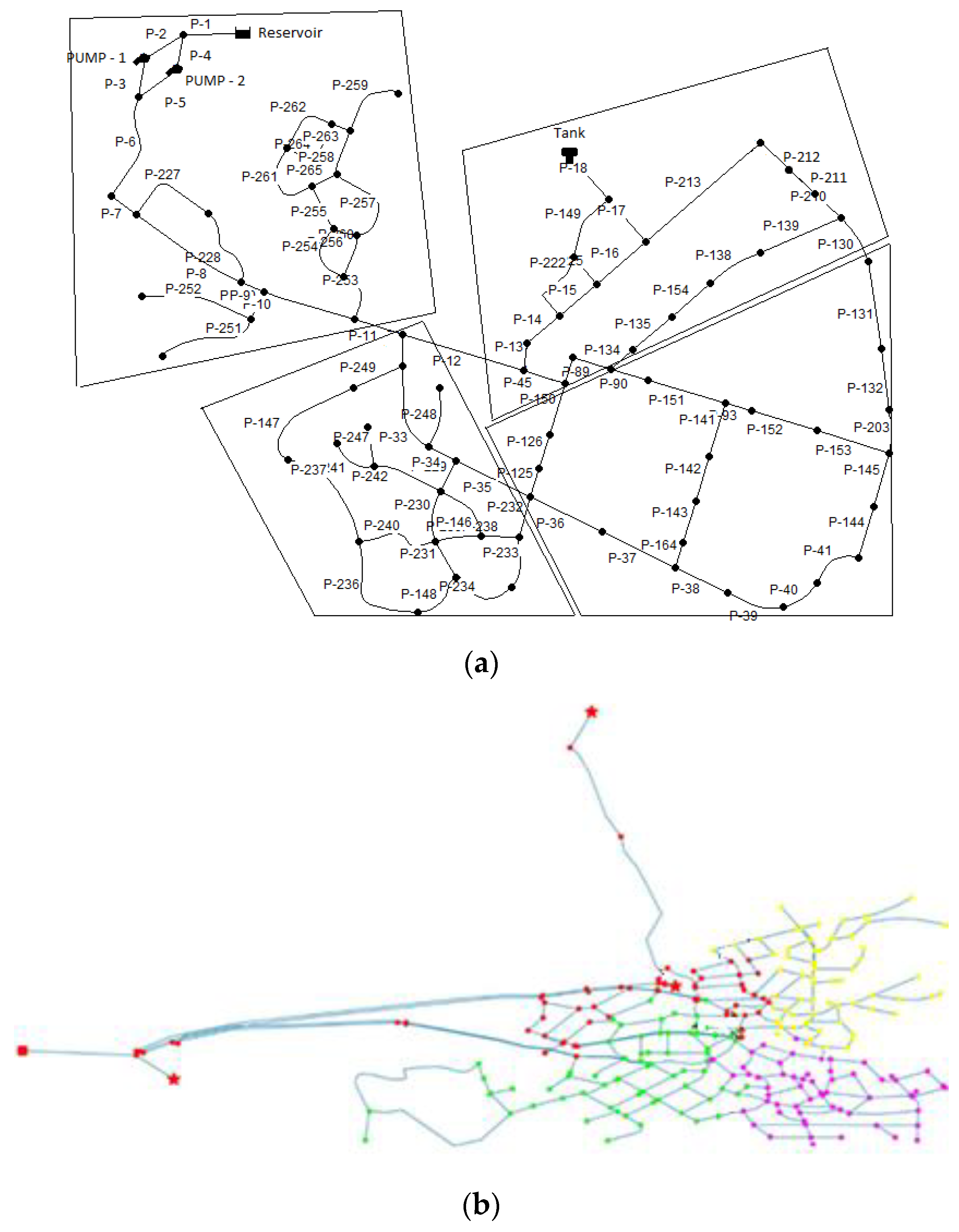
First, the RCB algorithm is applied for the Geometric Partition with n = 4 for both networks, where n is the number of partitions (Figure 4a,b).
3.2. Applying the Performing the Gaussian Mixture Model
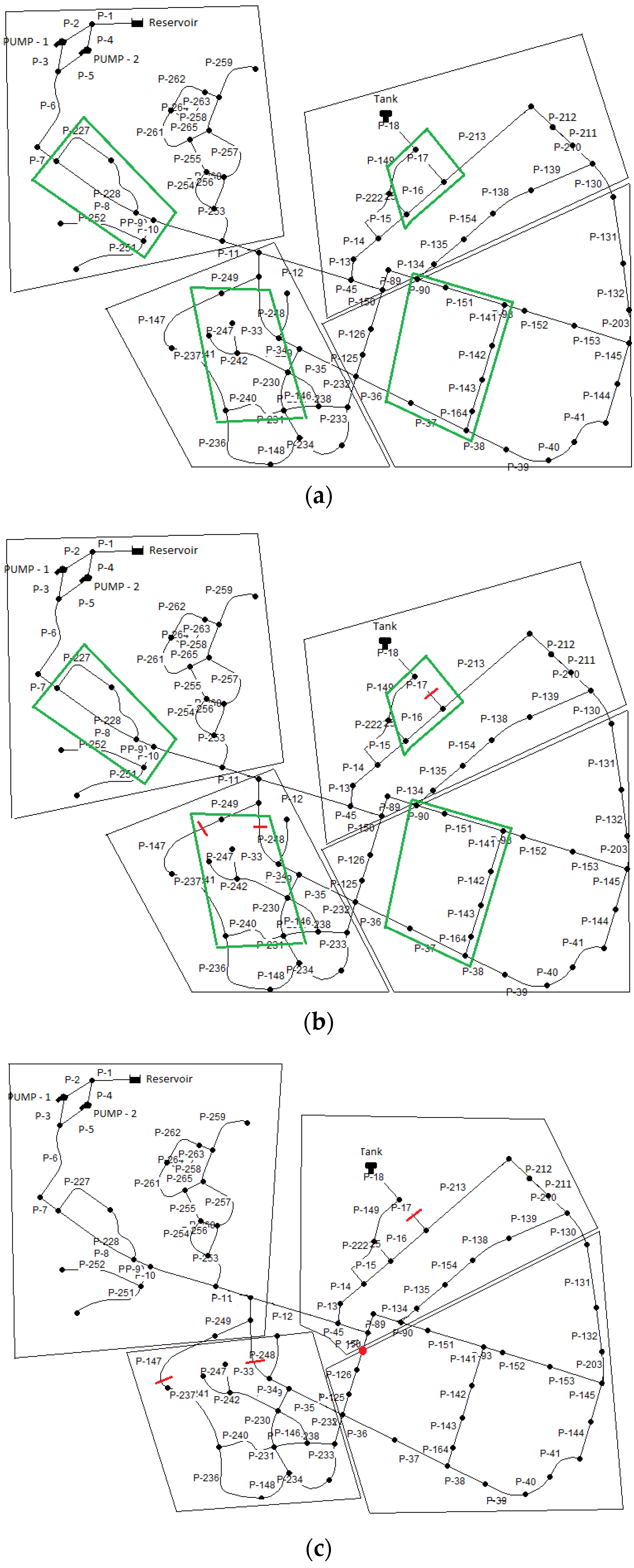
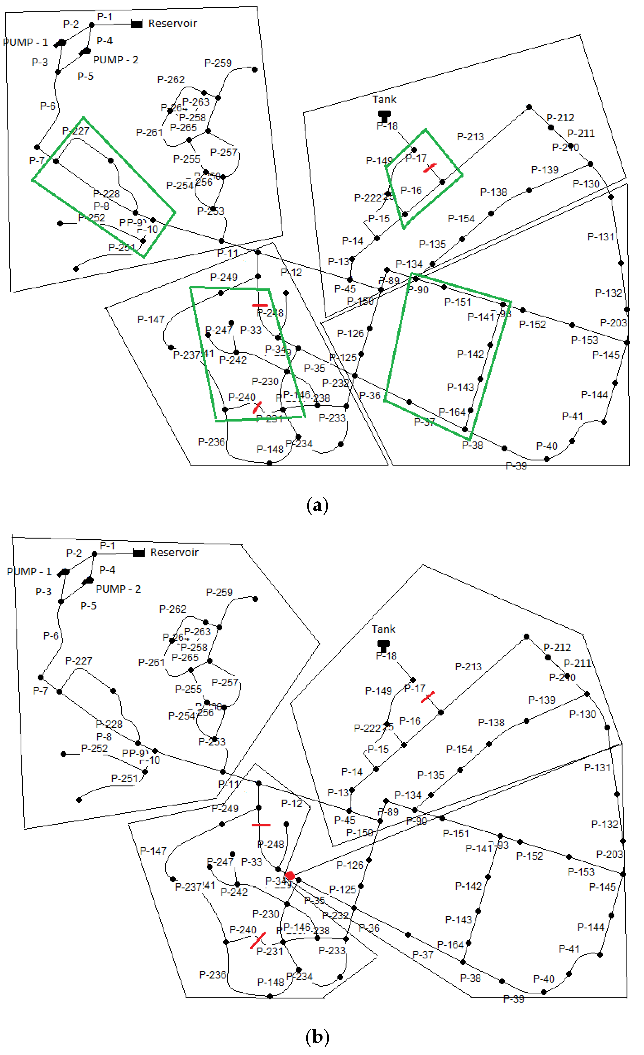
After applying the GMM-EM algorithm to the Net 22 and specifically to each sub-region created through the Geometric Partition, the clusters were formed (Figure 5a). The clusters having the highest mean average (μk) value, resulted by comparing the mean average value of each cluster generated, were marked in green. After placing an isolation valve on each pipe or a combination of them within the specific cluster, the total product Pressure × Demand for a period of the 24-h (PD) was checked. It should be noted that the parameters’ initial values and the number of clusters k were iteratively being set. The final selection was based on those that optimize the total product Pressure × Demand. In Figure 5b, the pipes selected by the model to be closed (P-17, P-33, and P-126) are noted with red lines. The initial value of the product Pressure × Demand before closing the pipes was 1,597,700 (psi × gpm), while after using isolation valves dropped to 771,360 (psi × gpm), thus reduced by 52.72%. At the same time, the average age of water was reduced by 5%, compared to its initial value (before the optimization) that was 41.31 h. The red circle indicates the pipe selected to install a Pressure Reducing Valve (PRV). Finally, the most critical junction is ‘J-90’ with a total pressure drop at 72.77% (Figure 5c). The initial average pressure value for the critical node is 109.7535 psi and the final is 29.8852 psi. Applying the GMM-EM algorithm, approximately five iterations until convergence were needed for each sub-region and 0.006 s of the total time was required.
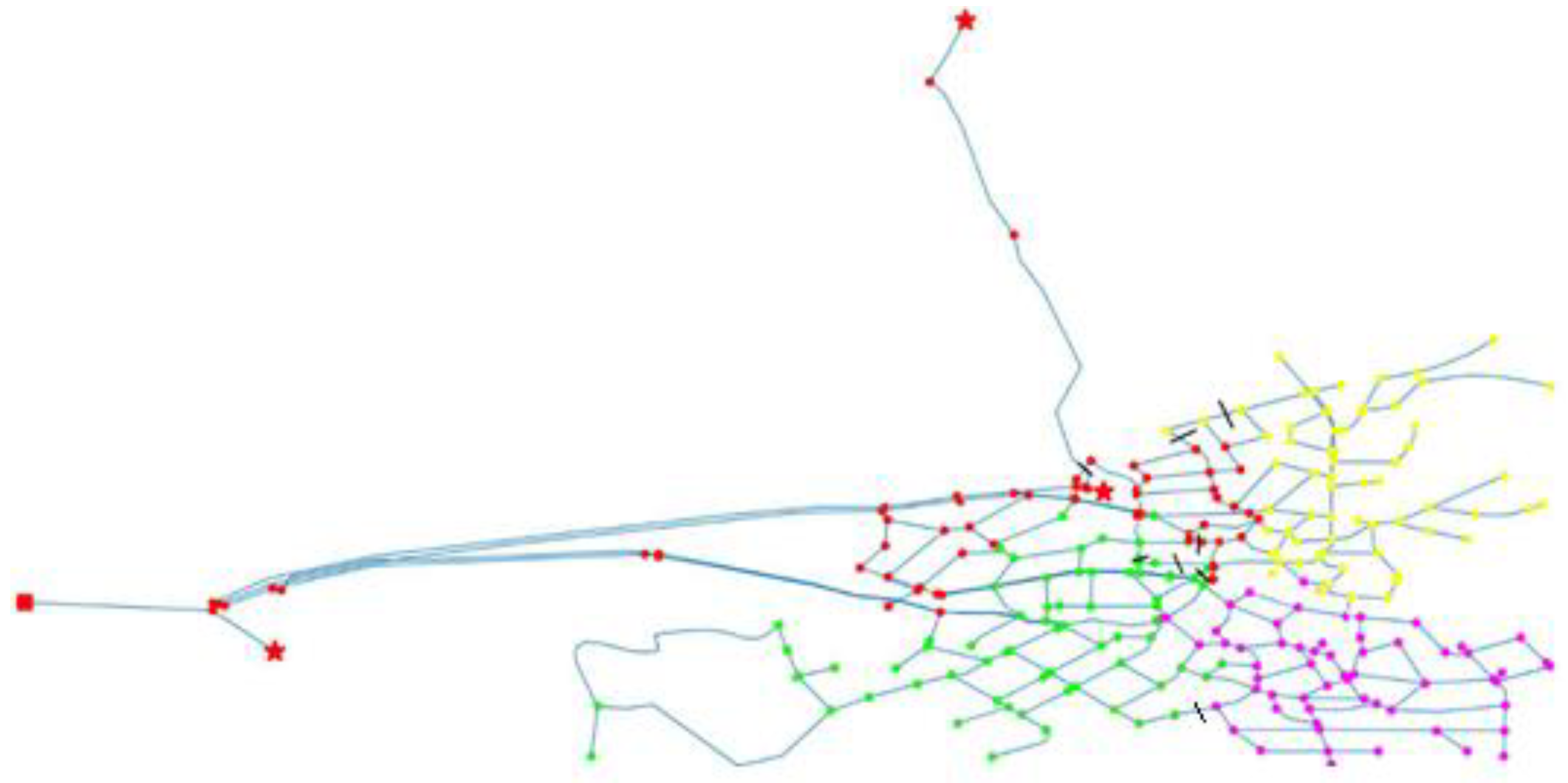
Figure 6 presents the separation achieved for the Aiani network. The pipes selected to be closed were 171, 134, 144, 138, 169, 332 and 142. The results showed a decrease of Pressure × Demand product by 34.70% with an initial value of 25,207,467.77 (psi × gpm), while the average water age was reduced by 5% starting with an initial value of 14.32 h. The optimum result, using the second objective function, was reached by placing an isolation valve at node 98 obtaining 5.22% Pressure × Demand product minimization (initial value: 78.5296 and final value: 74.4296). In this case, the average water age was reduced by 14.95%.
3.3. Applying the Student’s t-distribution Mixture Model
As already mentioned, after performing the Geometric Partitioning (GP) algorithm on the two aforementioned networks, well-defined, equivalent-sized areas were formed. For each sub-region, the SMM-EM algorithm was applied to the networks and the provided separations are presented in Figure 7a and Figure 8a, while the clusters having the highest average μk values are being marked with coloured shapes. Subseqently, each cluster was formed installing one or more isolation valves. The process was sequentially performed on all clusters, keeping the already intoduced isolation valves closed. The parameters’ initial values were iteratively set, taking into consideration the optimization of the result. Additionally, for comparison purposes, the same setup performed on the GMM-EM model with k = 4 was used here.
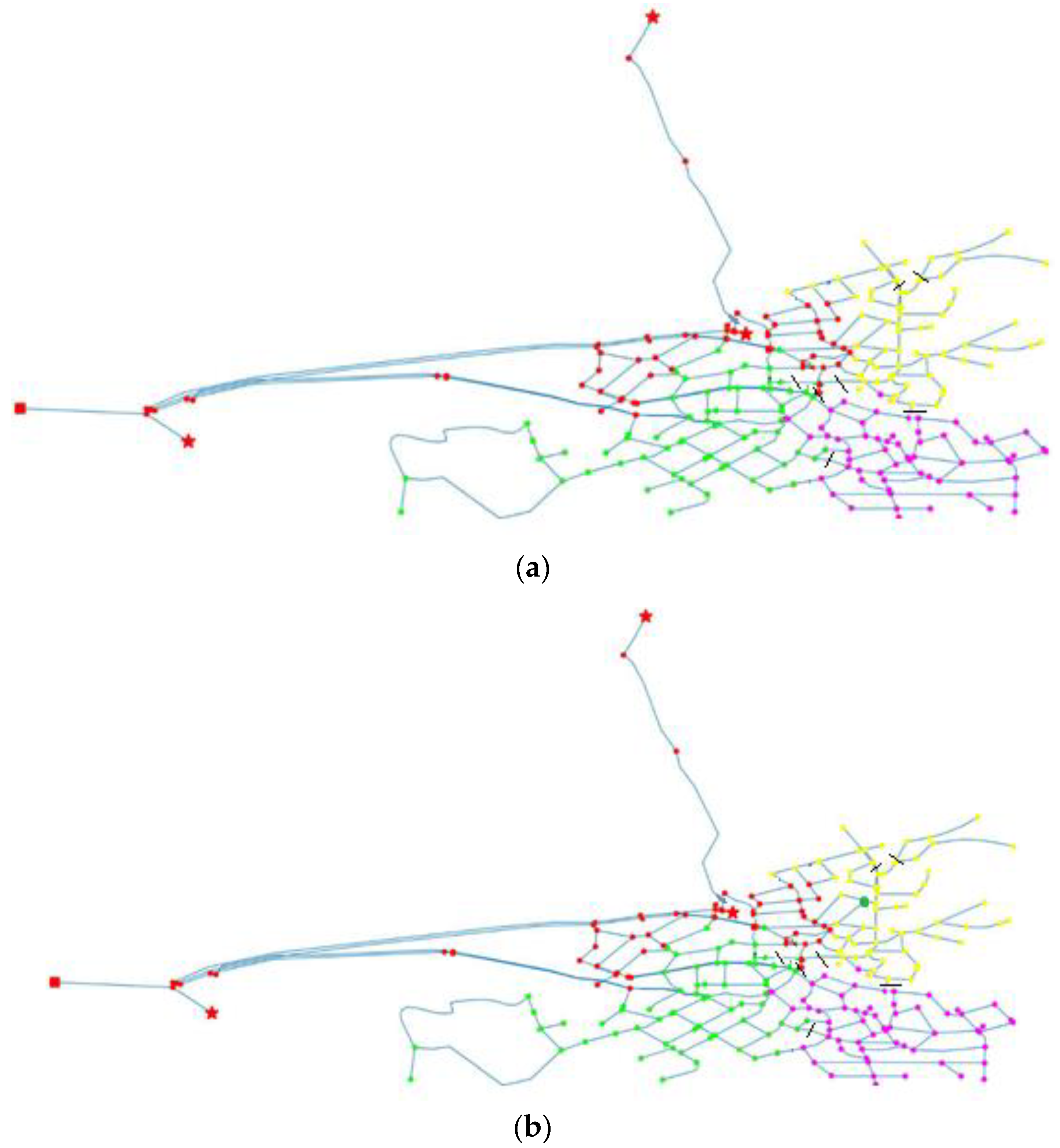
Through the SMM-EM model for the Net 22 network, three pipes were selected to be closed with red marks (Figure 7a). The total Pressure × Demand product was reduced by 76.52%, while the mean age of water was reduced by 8%. The red circle indicates the pipe proposed to host a PRV. Furthermore, the most critical junction is the ‘J-99’ one with initial value 129.3343 and a total pressure drop at 57.25%. Finally, considering the closed pipes through the proposed algorithm, a new separation of the network into DMAs was proposed (Figure 7b). It is obvious that the new separation is slightly altered regarding the partition created through the Geometric Partitioning algorithm. The SMM-EM algorithm requires approximately four iterations until convergence for each sub-region and 0.003 s. Therefore, after performing the proposed model on the Aiani network using the same setup as employed for the GMM-EM algorithm, seven pipes were selected to be closed (Figure 8a), reducing the total Pressure × Demand product by 43.69% and the average water age by 7.3%. Finally, the most critical junction is the ‘147’ one with initial value 68.8026 and a total pressure drop of 46.06% (Figure 8b).
3.4. Comparing the SMM-EM and GMM-EM Approaches to the Genetic Algorithm
To evaluate the performance of the proposed models, their results were compared with the Genetic Algorithm ones. Applying the Genetic Algorithm to the N22 network, eight different pipes were proposed to be closed, resulting in a reduced fitness function (PD product) by 16.69% and of the maximum water age by 3%. Thus, the reduction of the fitness function applying the Genetic Algorithm was 24.4% smaller compared to the respective one of the SMM-EM and GMM-EM models. Furthermore, the valves to needed when the Genetic Algorithm method is applied are almost double in number compared to those needed when the SMM-EM and GMM-EM models are applied. This is actually a significant drawback due to the huge installation cost. Finally yet importantly, the running time of the SMM-EM and GMM-EM was significantly reduced. Figure 7b and Figure 8a present the results of the comparison analysis between the three methods.
When the Genetic algorithm approach was applied to the Aiani network, the optimal scenario suggested eight pipes (IDs: 216, 171, 165, 155, 106, 332, 319, 287) to be closed. Following this suggestion, the fitness function (PD product) was decreased by 11.2%, while the water age by 0.5%.
4. Conclusions
Optimal pressure management (PM) in a WDN is a challenging task for water utility managers and researchers. The first basic step towards PM is the formation of DMAs. Different methodologies have been tested through the years focusing on many different aspects. The common goal is to optimize the formation of the DMAs in order to facilitate the efficient management of the system and reduce the average operating pressure even without installing Pressure Reducing Valves (PRVs). The current study attempted to present in brief a two-phase hybrid approach based on mixture models that can be applied for the optimal formation of DMAs. This approach used the following optimization criteria: a) Efficient pressure management in terms of minimizing the Pressure × Demand product (respecting the down limit of pressure, the water should be supplied to the customers’ meters, that is 29 psi based on the national legislation); and b) the water age in terms of the time the water remains inside the water pipes before reaching the customers’ taps as an indicator of how “fresh” the water is. At first, the networks are divided into sub-areas applying the method of Geometric Partitioning. Then, another algorithm runs in a parallel manner for every sub-area. Three algorithms were tested in order to compare their performance. These algorithms were the GMM-EM algorithm, the SMM-EM algorithm, and the Genetic Algorithm. Testing those three options, the best results came after applying the SMM-EM algorithm. Specifically, the best results regarding the optimization of the objective functions are those of the SMM-EM algorithm. Moreover, the computational time needed to run the networks applying the SMM-EM and the GMM-EM algorithms are almost identical and much less compared to the computational time needed when applying the Genetic algorithm. Concluding, the main contribution of the proposed models is the network’s complexity handling reduction, which leads to better control, and the simultaneous performance of the models on each region dramatically reducing the computational time needed. Especially in the real case of the Aiani network, which is a large network with great altitude variations between the network’s nodes, the proposed method performed impressively well. Finally, the hybrid approach resulted in an overall optimal placement of fewer (compared to the GA approach) PRVs, proving its suitability for sizeable networks and not only demo ones.
Author Contributions
V.K. defined the problem to be studied and provided the necessary data; S.C. and K.P. studied the problem, developed the algorithms, wrote the original paper; V.K. did the reviewing and final editing.
Funding
This research received no external funding.
Conflicts of Interest
The authors declare no conflict of interest.
References
- Di Nardo, A.; Di Natale, M. A heuristic design support methodology based on graph theory for district metering of water supply networks. Eng. Optim. 2011, 43, 193–211. [Google Scholar] [CrossRef]
- Herrera, M.; Canu, S.; Karatzoglou, A.; Pérez-García, R.; Izquierdo, J. An Approach to Water Supply Clusters by Semi-Supervised Learning. In Proceedings of the International Environmental Modelling and Software Society (IEMSS), Ottawa, ON, Canada, 5–8 July 2010. [Google Scholar]
- Izquierdo, J.; Herrera, M.; Montalvo, I.; Pérez-García, R. Division of Water Distribution Systems into District Metered Areas Using A Multi-Agent Based Approach. Commun. Comput. Inf. Sci. 2011, 50, 167–180. [Google Scholar]
- Deuerlein, J.W. Decomposition Model of a General Water Supply Network Graph. J. Hydraul. Eng. 2008, 134, 822–832. [Google Scholar] [CrossRef]
- Di Nardo, M.; Di Natale, G.F.; Santonastaso, V.G.; Tzatchkov, V.H. Water Network Sectorization based on genetic algorithm and minimum dissipated power paths. Water Sci. Technol. Water Supply 2013, 13, 951–957. [Google Scholar] [CrossRef]
- Tzatchkov, V.G.; Alcocer-Yamanaka, V.H.; Ortiz, V.B. Graph theory based algorithms for water distribution network sectorization projects. In Proceedings of the 8th Annual Water Distribution Systems Analysis Symposium, Cincinnati, OH, USA, 27–30 August 2006. [Google Scholar]
- Kadu, M.S.; Rajesh, G.; Bhave, P.R. Optimal design of water networks using a modified genetic algorithm with reduction in search space. J. Water Resour. Plan. Manag. 2008, 134, 147–160. [Google Scholar] [CrossRef]
- Chung, G.; Lansey, K. Application of the Shuffled Frog Leaping Algorithm for the Optimization of a General Large-Scale Water Supply System. Water Resour. Manag. 2009, 23, 797–823. [Google Scholar] [CrossRef]
- Atiquzzaman, M.; Liong, S.-Y. Using shuffled complex evolution to calibrate water distribution network. J. Civ. Eng. (IEB) 2002, 32, 111–119. [Google Scholar]
- Perelman, L.S.; Allen, M. Automated sub-zoning of water distribution systems. Environ. Model. Softw. 2015, 65, 1–14. [Google Scholar] [CrossRef]
- Di Nardo, A.; Di Natale, M.; Musmarra, D.; Santonastaso, G.F.; Tuccinardi, F.P.; Zaccone, G. Software for partitioning and protecting a water supply network. Civ. Eng. Environ. Syst. 2015, 33. [Google Scholar] [CrossRef]
- Brentan, B.M.; Campbell, E.; Meirelles, G.L.; Luvizotto, E., Jr.; Izquierdo, J. Social network community detection for DMA creation: Criteria analysis through multilevel optimization. Math. Probl. Eng. 2017, 2017, 9053238. [Google Scholar] [CrossRef]
- Diao, K.; Zhou, Y.; Rauch, W. Automated creation of district metered area boundaries in water distribution systems. J. Water Resour. Plan. Manag. 2013, 139, 184–190. [Google Scholar] [CrossRef]
- Williams, R.D. Performance of dynamic load balancing algorithms for unstructured mesh calculations. Concurr. Pract. Exp. 1991, 3, 457–481. [Google Scholar] [CrossRef]
- Simon, H.D. Partitioning of unstructured problems for parallel processing. Comput. Syst. Eng. 1991, 2, 135–148. [Google Scholar] [CrossRef]
- Kumar, G.S.; Raju, K.A.P.; Cpvnj, M.R.; Satheesh, P. Speaker recognition using GMM. Int. J. Eng. Sci. Technol. 2010, 2, 2428–2436. [Google Scholar]
- Figueiredo, M. Bayesian Image Segmentation Using Gaussian Field Prior. EMMCVPR 2005, 3757, 74–89. [Google Scholar]
- Fu, Z.; Wang, L. Color Image Segmentation using Gaussian Mixture Model and EM Algorithm. Multimed. Signal Process. 2012, 346, 61–66. [Google Scholar]
- Aroon, A.; Dhonde, S.B. Speaker Recognition System using Gaussian Mixture Model. Int. J. Comput. Appl. 2015, 130, 975–8887. [Google Scholar] [CrossRef]
- Lakshmanan, V.; Kain, J. A Gaussian Mixture Model Approach to Forecast Verification. Weather Forecast. 2010, 25, 908–920. [Google Scholar] [CrossRef]
- Chatzivasili, S.; Papadimitriou, K.; Kanakoudis, V.; Patelis, M. Optimizing the formation of DMAs in a water distribution network applying Geometric Partitioning (GP) and Gaussian Mixture Models (GMMs). Proceedings 2018, 2, 601. [Google Scholar] [CrossRef]
- Bernardo, J.M.; Smith, A.F.M. Bayesian Theory; John Wiley & Sons: Hoboken, NJ, USA, 2000. [Google Scholar]
- Reynolds, D.A.; Rose, R.C. Robust Text-Independent Speaker Identification using Gaussian Mixture Speaker Models. IEEE Trans. Acoust. Speech Signal Process. 1995, 3, 72–83. [Google Scholar] [CrossRef]
- Li, Z. Applications of Gaussian Mixture Model to Weather Observations. IEEE Geosci. Remote Sens. Lett. 2011, 8, 1041–1045. [Google Scholar] [CrossRef]
- Andrieu, C.; Freitas, N.D.; Doucet, A.; Jordan, M.I. An Introduction to MCMC for Machine Learning. J. Mach. Learn. 2003, 50, 5–43. [Google Scholar] [CrossRef]
- Xu, L.; Jordan, M.I. On Convergence Properties of the EM Algorithm for Gaussian Mixture. Neural Comput. 1996, 8, 129–151. [Google Scholar] [CrossRef]
- Gerogiannis, D.; Nikou, C.; Likas, A. The mixtures of Student’s t-distributions as a robust framework for rigid registration. Image Vis. Comput. 2009, 27, 1285–1294. [Google Scholar] [CrossRef]
- Korkana, P.; Kanakoudis, V. Forming district Metered Areas in a water distribution Network using Genetic algorithms. Procedia Eng. 2016, 162, 511–520. [Google Scholar] [CrossRef]
Figure 1.
Dividing a graph with the help of RCB in equal sub-domains.

Figure 2.
A Student’s t-distribution (μ = 0, σ = 1) for various degrees of freedom. As ν > the distribution tends to a Gaussian. For small values of ν, the distribution has heavier tails than a Gaussian [22].
Figure 2.
A Student’s t-distribution (μ = 0, σ = 1) for various degrees of freedom. As ν > the distribution tends to a Gaussian. For small values of ν, the distribution has heavier tails than a Gaussian [22].

Figure 3.
(a) Net 22, (b) Aiani Network.

Figure 4.
Forming the networks’ DMAs: (a) Net 22 and (b) Aiani into sub-regions using Geometric Partitioning.
Figure 4.
Forming the networks’ DMAs: (a) Net 22 and (b) Aiani into sub-regions using Geometric Partitioning.

Figure 5.
(a) The clusters with the highest average value for each sub-region using GMM-EM (green contour), (b) the clusters and the pipes in which isolating valves are installed are colored in red and (c) splitting of Net 22 into DMAs and the pipes with the red circle denote the selected pipes for PRV installation.

Figure 6.
Separating Aiani network in DMAs marked with different colors and with black marks the pipes where isolated valves were placed.
Figure 6.
Separating Aiani network in DMAs marked with different colors and with black marks the pipes where isolated valves were placed.

Figure 7.
(a) The clusters with the highest average value for each sub-region using SMM-EM (green contour) and the pipes in which isolating valves are installed (red), (b) the division of the network in DMAs and the selected pipes for PRV installation (red circle).
Figure 7.
(a) The clusters with the highest average value for each sub-region using SMM-EM (green contour) and the pipes in which isolating valves are installed (red), (b) the division of the network in DMAs and the selected pipes for PRV installation (red circle).

Figure 8.
(a) The pipes chosen for closing using SMM-EM (black lines), and (b) the selected junction for PRV installation (green circle).
Figure 8.
(a) The pipes chosen for closing using SMM-EM (black lines), and (b) the selected junction for PRV installation (green circle).


Table 1.
Reduction rates based on the various values of k (number of clusters) for both networks.
| Number of Clusters (k) | Net 22 Network | Aiani Network | ||||
|---|---|---|---|---|---|---|
| P × D | Age | Critical Node (Pressure > 29 psi) | P × D | Age | Critical Node (Pressure > 29 psi) | |
| 2 | 24.31% | 0.23% | J-149 (57.25%) | 9.16% | 2.01% | 197 (19.11%) |
| 3 | 15.56% | 0.95% | J-150 (24.68%) | 11.22% | 1.52% | 207 (20.20%) |
| 4 | 52.12% | 5% | J-90 (72.77%) | 34.70% | 5% | 157 (55.82%) |
| 5 | 45.87% | 3.21% | J-28 (70.10%) | 21.19% | 2.28% | 179 (38.98%) |
| 6 | 43.21% | 4.18% | J-29 (64.34%) | 20.57% | 3.99% | 188 (35.38%) |
© 2019 by the authors. Licensee MDPI, Basel, Switzerland. This article is an open access article distributed under the terms and conditions of the Creative Commons Attribution (CC BY) license (http://creativecommons.org/licenses/by/4.0/).
Share and Cite
MDPI and ACS Style
Chatzivasili, S.; Papadimitriou, K.; Kanakoudis, V. Optimizing the Formation of DMAs in a Water Distribution Network through Advanced Modelling. Water 2019, 11, 278. https://doi.org/10.3390/w11020278
AMA Style
Chatzivasili S, Papadimitriou K, Kanakoudis V. Optimizing the Formation of DMAs in a Water Distribution Network through Advanced Modelling. Water. 2019; 11(2):278. https://doi.org/10.3390/w11020278
Chicago/Turabian StyleChatzivasili, Stavroula, Katerina Papadimitriou, and Vasilis Kanakoudis. 2019. "Optimizing the Formation of DMAs in a Water Distribution Network through Advanced Modelling" Water 11, no. 2: 278. https://doi.org/10.3390/w11020278
Note that from the first issue of 2016, this journal uses article numbers instead of page numbers. See further details here.