Climate Change Impact on Flood Frequency and Source Area in Northern Iran under CMIP5 Scenarios

Abstract

This study assessed the impact of climate change on flood frequency and flood source area at basin scale considering Coupled Model Intercomparison Project phase 5 General Circulation Models (CMIP5 GCMs) under two Representative Concentration Pathways (RCP) scenarios (2.6 and 8.5). For this purpose, the Soil and Water Assessment Tool (SWAT) hydrological model was calibrated and validated for the Talar River Basin in northern Iran. Four empirical approaches including the Sangal, Fill–Steiner, Fuller, and Slope-based methods were used to estimate the Instantaneous Peak Flow (IPF) on a daily basis. The calibrated SWAT model was run under the two RCP scenarios using a combination of twenty GCMs from CMIP5 for the near future (2020–2040). To assess the impact of climate change on flood frequency pattern and to quantify the contribution of each subbasin on the total discharge from the Talar River Basin, Flood Frequency Index (FFI) and Subbasin Flood Source Area Index (SFSAI) were used. Results revealed that the projected climate change will likely lead to an average discharge decrease in January, February, and March for both RCPs and an increase in September and October for RCP 8.5. The maximum and minimum temperature will likely increase for all months in the near future. The annual precipitation could increase by more than 20% in the near future. This is likely to lead to an increase of IPF. The results can help managers and policy makers to better define mitigation and adaptation strategies for basins in similar climates.

1. Introduction

Floods are complex natural hazards that can cause massive social and economic damage [1]. According to the Intergovernmental Panel on Climate Change (IPCC), recent climate change has had a significant impact on the magnitude and frequency of extreme hydrological events in many regions of the world [2]. Flood frequency, however, differs according to local climate and watershed characteristics in different regions of the world [3]. Therefore, investigation of climate change impact at a basin scale is essential to mitigate negative societal impacts.

The uncertainty associated with climate change effects on extreme events is a challenging issue at both local and regional scale [4]. On the one hand, the climate change impacts on river discharge in Iran show a significant change in flood properties for nearly half of the country [5]. This highlights the importance of climate change impact assessment for extreme events as direct influence on human life, economy, and environment [6]. On the other hand, the frequency and magnitude of floods are also affected by gradual land use changes that may exacerbate the situation [7,8]. For example, urbanization and urban sprawl are likely to increase flood risk. Therefore, assessing the impact of present and future climate also requires estimation of future land use for achieving appropriate adaptation policy [9,10,11]. In this regard, hydrological modeling plays an important role in simulating possible future changes and their impact, hence helping to determine proper watershed management practices [12]. In this respect, the SWAT model has emerged as one of the best available hydrological models for investigating the streamflow response to climate change [13].

In order to simulate effects of a future climate, output from global coupled atmospheric-ocean General Circulation Models (coupled GCMs) is used as input to hydrological models [14]. The number of GCMs available for climate change projections is developing rapidly. In this regard, the Coupled Model Intercomparison Project phase 5 (CMIP5) GCMs, which were introduced in the fifth IPCC report with enhancement in the physical description and numerical algorithms, have recently become accessible. In these models, a new set of scenarios—namely Representative Concentration Pathways (RCPs)—are used [15,16] that include upper and lower limits of greenhouse gas emission scenarios.

Among various methods for flood-risk characterization, flood magnitude and frequency analyses are recognized as essential variables in flood-risk management studies [3]. Changes in frequency and intensity of flood events can lead to severe impacts on different aspects of human life including environmental, social, and economic conditions [17]. In this regard, flood frequency analysis is a statistical approach that provides a probability model using annual flood peaks during a given period [18]. Having an insight regarding the probability of the peak and magnitude of the flood enables water professionals to adopt and implement proper flood management. In addition, this may assist planners to design hydraulic structures to reduce flood impact in flood-prone areas [19].

Many studies have confirmed that the spatial rainfall pattern significantly governs the flood characteristics [20]. Therefore, determining the flood response, magnitude, and frequency from rainfall is necessary for selection of the best management practices [21]. The implementation and cost of structural and non-structural flood measures in large flood-prone non-perennial river basins are challenging issues. One way to deal with this is to minimize the cost of flood damages by considering downstream flood-threatened areas with the most sensitive subbasins instead of the entire basin [12,20,22]. For this, Saghafian and Khosroshahi (2005) proposed a Unit Flood Response (UFR) approach to identify and rank flood-threatened subbasins in quantitative terms related to flood source area. This can be conducted based on the different contribution from each subbasin to the total river discharge. Accordingly, flood management practices may be primarily directed toward such areas to obtain optimum spatial planning of the basin [20].

In view of the above, the potential impact of climate change on flood risk can be assessed using a coupled climate-hydrological model approach [11,23,24,25]. Therefore, in this study, the Soil and Water Assessment Tool (SWAT) was used to estimate Flood Frequency Index (FFI) in the Talar River Basin located in the south Caspian Sea region. The objective was to assess the hydrological response, i.e., flood magnitude and frequency, due to future changes in climate and land use. The region contains fast-growing settlements that are vulnerable to climate change [5]. This, in turn, requires new policies to protect land and natural resources as well as human lives against future flood hazard. Talar is one of the major rivers in the region, and a critical situation has been reached due to unmanaged development of its riverside areas [26]. For this purpose, we evaluated the potential impact of climate change on flood frequency pattern and flood source area in the Talar River Basin. The study was carried out following five methodological steps: (1) a SWAT model was calibrated at a daily time step for the basin, (2) an ensemble of twenty regional CMIP5 GCMs was produced and downscaled using a statistical downscaling technique, Long Ashton Research Station Weather Generator (LARS-WG), was used to project precipitation and temperature under RCP2.6 and RCP8.5 scenarios for the 1984–2005 period, (3) an Instantaneous Peak Flow (IPF) estimation method was used to estimate the present and near future discharge, (4) changes of flood frequency were assessed and compared within the subbasins by Flood Frequency Index (FFI) calculation for present and near future periods, and (5) Subbasin Flood Source Area Index (SFSAI) and the contribution of each subbasin to total flooding for the present and near future were determined and ranked.

2. Materials and Methods

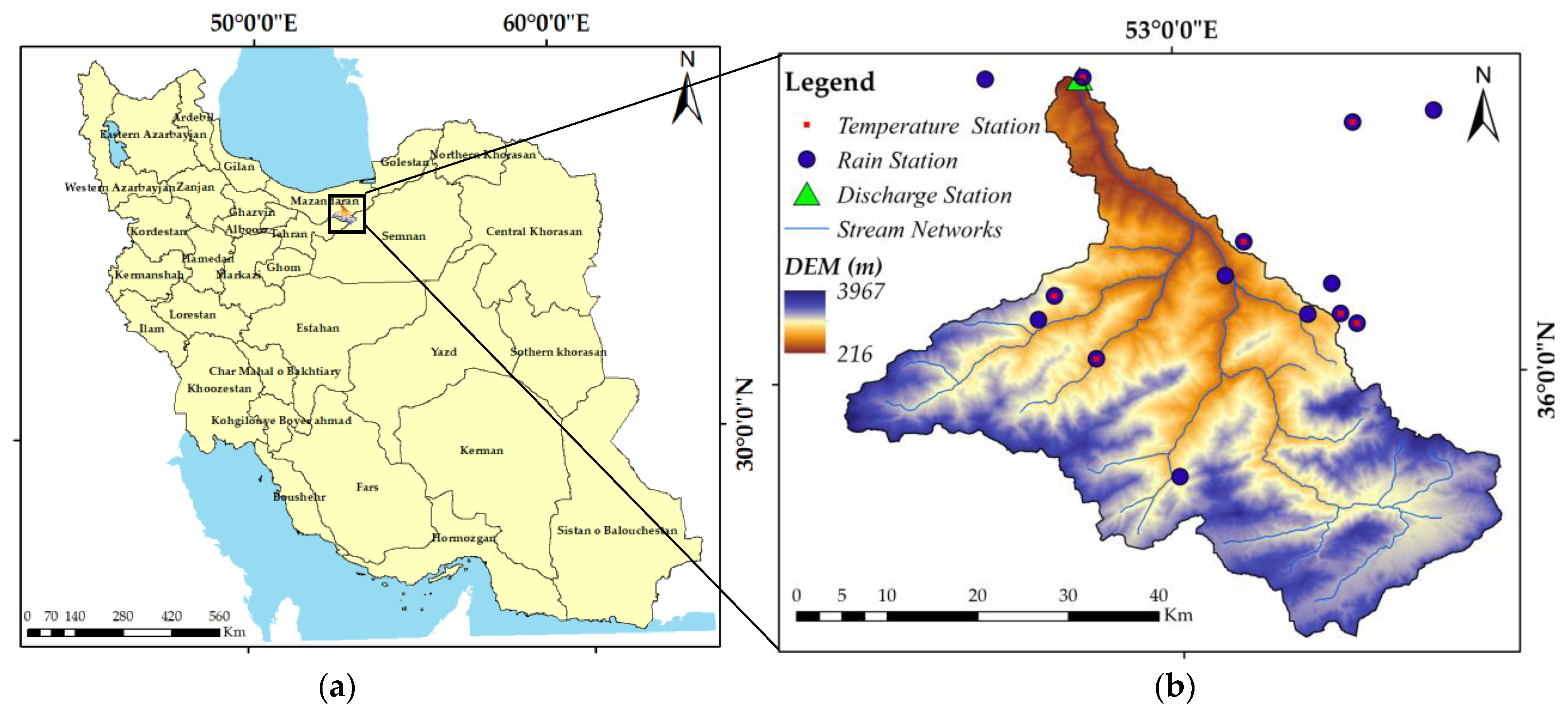
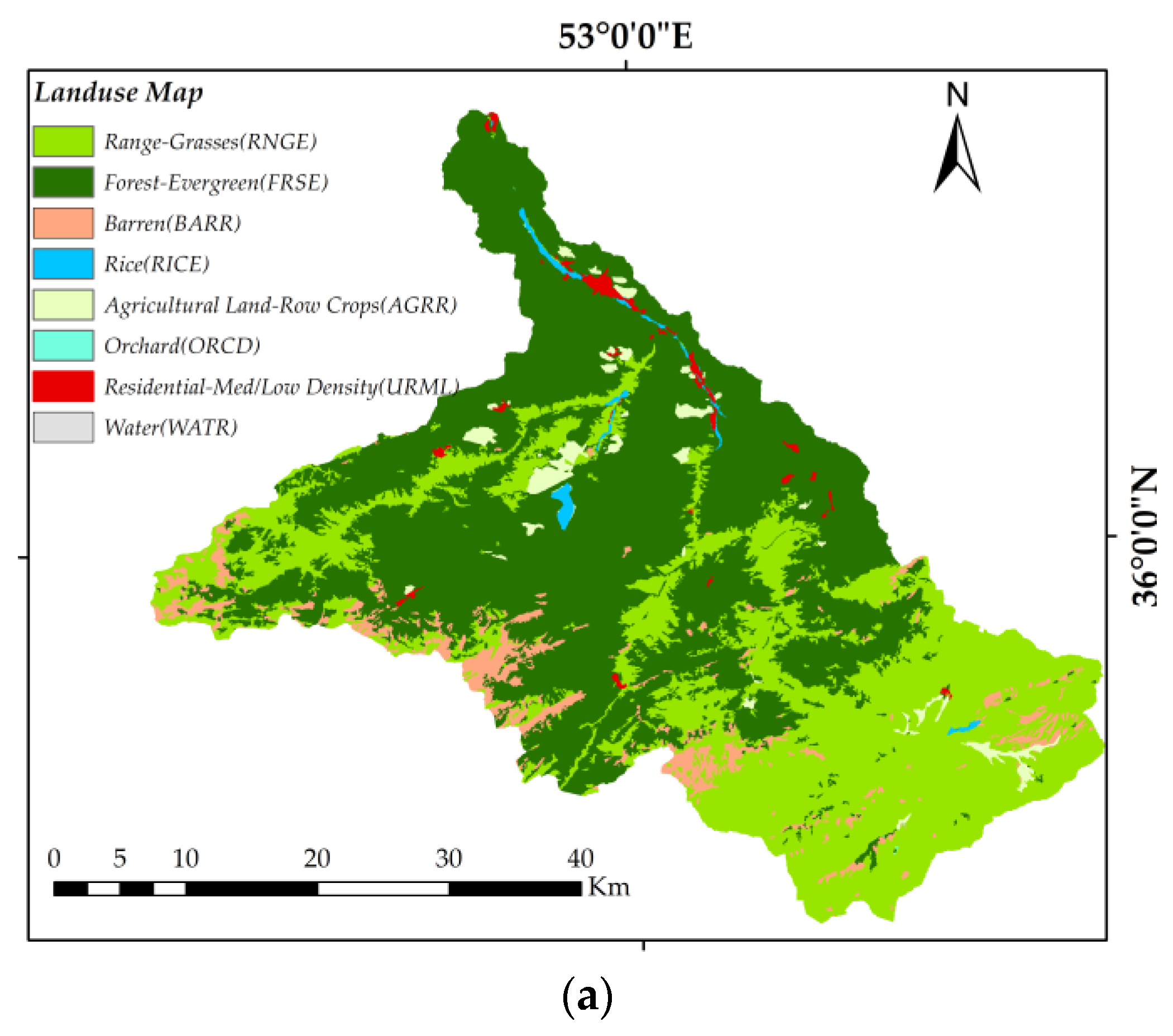
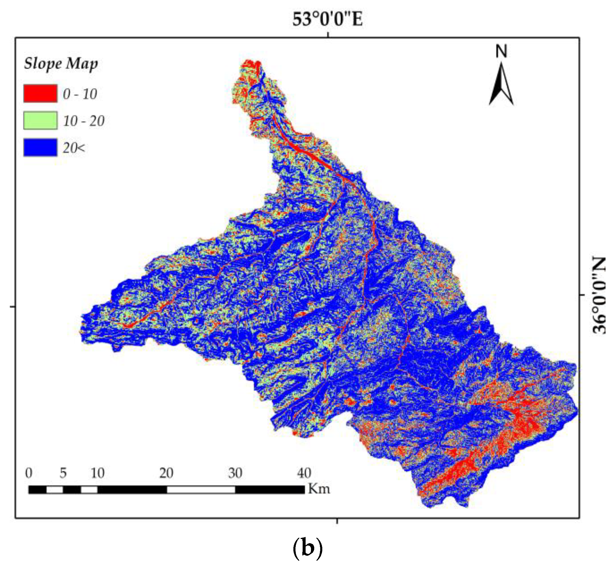
2.1. Study Area

Talar River Basin is located in the mountainous region of the Mazandaran Province in northern Iran close to the Caspian Sea and covering an area of 1727 km² [27,28]. The basin constitutes one of the subbasins of Haraz and Gharasou watersheds located between 52°35′ to 53°25′ East and 35°45′ to 36°20′ North [29] (Figure 1). The altitude ranges between 216 and 3967 m above mean sea level. The average slope of the basin, main river channel, and the length of the main river channel are 16%, 13%, and 100 km, respectively [30]. The annual average precipitation and temperature are 610 mm and 11 °C, respectively, and hence, the basin is considered as semi-humid [29]. Significant land uses in the area are forest (50%), rangeland (30%), and agriculture and urban areas (20%). The dominating crops are rice and wheat constituting about 23% of the agricultural land. Further, the soil texture of the Talar Basin is mainly silty loam, silty clay, loamy clay, and clayey loam [31].

2.2. Climate Change Assessment

Climate change impact on hydrological processes depends on the projected future climate scenarios provided by climate models [32]. In this study, twenty CMIP5 GCMs for the lowest (RCP 2.6) and highest (RCP 8.5) emission scenario were used as input for future climate assessment. In this regard, RCP 2.6 represents a mitigation scenario leading to a low forcing level (peak in radiative forcing at 3 W/m² before 2100 and reaching 2.6 W/m² by 2100) and RCP 8.5 a high baseline emission scenario (rising radiative forcing pathways leading to 8.5 W/m² by 2100) [33,34].

Many studies have used climate change models to simulate the current climate and its future evolution under different greenhouse gas and aerosol scenarios [35]. Despite a large number of improved GCMs for climate change projections, uncertainty remains regarding the future climate [36]. One way to reduce uncertainty in climate projections is to use an ensemble of multi-model GCMs. Multi-model GCMs ensembles are used to obtain a spectrum of possible future outcomes. In this study, we calculated the median value of climate scenarios derived from twenty CMIP5 GCMs. As these climate projections are defined at a coarse grid (approximately 150–300 km), they cannot be implemented as input to the hydrological model for climate change impact assessment. Therefore, several statistical or dynamical downscaling approaches are used that allow researchers to gain a higher spatial and temporal resolution required for hydrological applications [32]. LARS-WG developed by Semenov and Barrow [37] is a well-known stochastic weather generator for downscaling and producing daily time series of climate variables, i.e., precipitation, temperature, and solar radiation. The model uses observed weather data for a baseline period and computes the changes in climate parameters [38]. More detailed information about the procedure of this downscaling approach is described in Reference [39].

In this study, the output from the climate scenarios was used as input to the calibrated SWAT model to provide an assessment of expected changes in daily discharge for the near future (2020–2040). Therefore, data from twenty climate models including precipitation, minimum and maximum temperature for the historical (1984–2005) and near future (2020–2040) period covering the study area were downloaded from the CMIP5 GCMs data archive (http://cmip-pcmdi.llnl.gov/cmip5/index.html).

Due to the fact that the LARS-WG model has not yet been adopted to all CMIP5 GCMs scenarios, the delta change method was used as a downscaling approach to adapt CMIP5 GCMs output for the watershed-scale analysis and hydrological modeling [40]. The delta change can be calculated based on a monthly change factor for precipitation and temperature [23]. These change factors were used as first scenarios in LARS-WG to generate future time series of precipitation and maximum and minimum temperature. Consequently, the monthly averages for 1984–2005 and 2020–2040 were used as a baseline for present and near future period analyses, respectively. The difference between observed precipitation and temperature and those of the twenty CMIP5 outputs during 1984–2005 was calculated according to [40]:

$$\Delta P_i=\frac{{\overline{P}}_{GCM.fut, i}}{{\overline{P}}_{GCM.his, i}}$$

(1)

$$\Delta T_{ma{x}_i}={\overline{T}}_{ma{x}_{GCM.fut, i}}-{\overline{T}}_{ma{x}_{GCM.his, i}}$$

(2)

$$\Delta T_{mi{n}_i}={\overline{T}}_{mi{n}_{GCM.fut, i}}-{\overline{T}}_{mi{n}_{GCM.his, i}}$$

(3)

where, $\Delta P_i$, $\Delta T_{ma{x}_i}$, and $\Delta T_{mi{n}_i}$ are the change in precipitation and maximum and minimum temperature for ith month (January–December). ${\overline{T}}_{maxGCM.fut, i}$ and ${\overline{T}}_{maxGCM.his,i}$ are the long-term average of ith month for the maximum temperature for a future and historical (present) period, respectively. ${\overline{T}}_{minGCM.fut, i}$ and ${\overline{T}}_{minGCM.his,i}$ are the long-term average of ith month for minimum temperature in the future and historical (present) period, respectively.

Various statistical checks such as student’s t-test, F-test, and chi-square test are adopted in the LARS-WG environment to compare calculated and observed weather data for the investigated period [37]. Precipitation and maximum and minimum temperature for each station were estimated using LARS-WG. Time series for the near future (2020–2040) for each RCP scenario were calculated using the observed datasets as input to LARS-WG [6]. Therefore, the generated precipitation and maximum and minimum temperature for the near future were used as input weather data to the SWAT model as described below.

2.3. Hydrological Modeling (SWAT)

Hydrological modeling plays a vital role in the analysis of water resources subjected to climate change, especially when attempting to simulate future hydrological impact [41]. Such models have been widely used in climate change assessment studies to build a linkage between climate variables and river discharge [42]. The SWAT model is a physically based semi-distributed model that has been developed to simulate flow and predict the impact of climate change and management practices [13,43,44]. The SWAT model can be applied at various scales ranging from basin to continental [45]. The model is separated into two parts for hydrological simulations; a land phase and a routing phase. The land phase governs the amount of water, sediment, nutrients, and pesticide loadings to the main channel in each subbasin. The routing phase considers the movement of water, sediments, nutrients, and component of the hydrological cycle [46]. The land phase of the hydrological cycle in SWAT is based on the water balance equation:

$$S{W}_t=S{W}_0+{\displaystyle \sum }_{i-1}^t(R_{day}-Q_{surf}-E_a-w_{seep}-Q_{gw})$$

(4)

where SW_t and SW₀ are the final and initial soil water content for day i, respectively, R_day is rainfall that reaches soil surface, Q_surf is surface runoff, E_a is evapotranspiration, w_seep is interflow, and Q_gw is base flow [47]. It is noted that the ability of this model to generate discharge at a monthly time step for the studied basin has been tested by Kavian et al. [27].

2.3.1. SWAT Input Data

A Digital Elevation Model (DEM) of the Talar River Basin with 30 m resolution was used to generate slope data (Figure 2). The soil map was obtained from the Forest, Rangeland, and Watershed Management Organization (FRWO) of Iran [27]. To generate the land use map, Landsat 8 images (Operational Land Imager; OLI) covering the study area were used. The training data points for each land use were validated by field visits and Google Earth application. The land use map was then produced in an Evni 5.3 environment. Finally, eight types of land use were detected (Figure 2) and fed into the land use look-up table in the SWAT model. In addition, 58 types of soils with different physical and chemical properties were used [27]. Daily rainfall data from 14 stations and maximum and minimum temperature data from 7 stations for the studied basin were collected from the Iranian Meteorological Organization (IMO) and the Iran Water Resources Management Company (IWRMC). Precipitation, maximum and minimum temperature, relative humidity, solar radiation, and wind speed were then used to create the weather generator input file.

Due to intense agricultural activity and water use, estimation of evapotranspiration is a crucial component of the water balance. The agricultural practices in the basin such as irrigation schedule (amount and interval), tillage, cropping, and harvesting periods were gathered from FRWO. Accordingly, agricultural management and crop yield information were implemented in the model for accurate calculation of evapotranspiration [45,48]. It should be mentioned that all spatial data sets were resampled into DEM grid size with 30 m resolution and daily time scale for the 2008–2016 period. To calculate conditions for the future period, historical data were replaced by the projected precipitation and temperature. Then, the SWAT model was run to automatically generate other weather inputs including solar radiation, relative humidity, and wind speed to produce future flooding occurrence under the two climate scenarios [49].

2.3.2. SWAT Model Set Up

To set up and parameterize the hydrological model, Arc SWAT 2012 interface was used as an extension tool in the Arc GIS 10.4 environment. As a first step, the basin was divided into subbasins using the basin delineation tool and further sub-divided into unique land use, soil, and slope characteristics as Hydrological Response Units (HRUs) by adding layers of land use and soil maps with defined slope ranges [50]. DEM and stream network maps were fed into the SWAT model as well as the river discharge locations. Note that some additional adjustment, i.e., river network and observed outlet location, were applied to facilitate the calibration process [51]. In addition, look-up tables were used to re-classify land use and soil maps, connected to the SWAT database. The classified slope and soil map was introduced to the model, and ten elevation bands were determined to adjust the temperature and rainfall based on subbasin elevation variation. To create fewer HRUs, a 10% threshold for land use, soil type, and slope were determined [52]. Therefore, based on the DEM data and accurate flow routing, the Talar River Basin was divided into 21 subbasins by a threshold drainage area of 3453 km². The subbasins were then further divided into 1110 HRUs based on land use, slope, and soil maps in the Arc SWAT 2012 interface. The weather station data (Figure 1b) including daily precipitation, maximum and minimum temperature, and wind speed were imported to the model for the 2008–2016 period. The stream networks and observed outlet location were corrected using Arc Bru Tile extension in Arc GIS 10.4 by providing a Bing map. Potential evapotranspiration from the Penman–Monteith method was calculated [53]. To run the SWAT model at a daily time step, a two-year period (2008–2009) was selected as a warm-up period, and 2010–2013 and 2014–2016 were considered for calibration and validation periods, respectively.

2.3.3. Calibration of the Model (SWAT-CUP)

Hydrological models substantially rely on several effective parameters, which are varying widely in space and time while transforming input data to the output variables. These parameters inherently govern the hydrological cycle and hence model performance to accurately reflect natural conditions. Due to the lack of observed data, the number of parameters can be reduced during the calibration process by sensitivity analysis. This was carried out by eliminating the parameters for which the model did not show sensitivity. This, in turn, lead to an efficient fitting of sensitive parameters [54]. For this, SWAT-CUP (Calibration and Uncertainty Procedures) [45] has been widely applied as helpful tool to perform parameterization, sensitivity analysis, uncertainty analysis, calibration, and validation of hydrologic variables [43]. Among five different calibration algorithms in SWAT-CUP, the Sequential Uncertainty Fitting 2 (SUFI-2) approach has been shown to be an efficient algorithm for model calibration [45,55]. Accordingly, parameter sensitivity analysis, calibration, and validation were conducted in SWAT-CUP using the SUFI-2 algorithm [50]. For calibration and validation procedures, daily discharge data at the Shirgah station located at the outlet of the Talar River Basin (Figure 1) were acquired from the Mazandaran Regional Water Authority for the 2010–16 period.

2.3.4. Evaluation of Model Performance

The SWAT simulation performance and accuracy were evaluated through calculation of the coefficient of determination (R²) and Nash–Sutcliffe coefficient (NSE) between observed and simulated discharge for the calibration and validation periods. R² expresses the degree of collinearity between simulated and observed data, which varies from 0 to 1. The higher the R² and NSE, the better agreement between simulated and observed discharge [50,56].

2.4. Flood Frequency Assessment

2.4.1. IPF Estimation Methods

Flood frequency analysis was based on annual flood time series [57]. In flood-risk management and design of the hydraulic structures, the use of Instantaneous Peak Flow (IPF) curve is suggested to prevent underestimation of daily peak flow [58]. In this study, four empirical approaches including Fuller [59], Sangal [60], Fill–Steiner, and slope-based [58] methods were used to estimate the IPF from daily discharge. Then, the best method was chosen based on the performance indices including R², NSE, Root Mean Squared Error (RMSE), and Mean Absolute Error (MAE). The easy-fit application was used to select the best fit distribution to annual maximum flow discharge (35 years) using the Goodness Of Fit (GOF) test. The GOF test shows how well the selected distribution fits the daily discharge data. Accordingly, the annual maximum discharge was extracted for the present period. Then, the IPF was estimated using the four empirical methods, and the best IPF estimation method was selected. After this, the flood frequency for a return period of 2 to 200 years was estimated using the IPF time series at the main outlet of the basin.

2.4.2. Flood Frequency Index (FFI)

To quantify the impact of climate change on flood frequency distribution, the Flood Frequency Index (FFI) was calculated based on the simulated daily discharge flow rate at each subbasin’s outlet for both present and future periods. The FFI was calculated using:

$$FFI=\frac{{{\displaystyle \sum }}_{i=1}^{N}FFi}{N}$$

(5)

where FFi is the number of flood events in a water year i calculated as the fraction of days with flow above or equal a given threshold. A two-year flood threshold was used for counting the number of flood events in each subbasin. N is the total number of years in the simulation period [49].

2.4.3. Subbasin Flood Source Area Index (SFSAI)

The unit flood response was used to determine and rank different subbasins regarding their contribution to flood generation at the downstream area [61]. Previous studies have used this approach with hydrological models such as ModClark [62] and HEC-HMS [63]. For this purpose, SWAT was used to determine the Subbasin Flood Source Area Index (SFSAI). This approach can also be applied to quantify the contribution of subbasins to the peak flow and determine subbasins that are primary contributors to generating flood [64]. In this context, individual subbasins were systematically removed in each simulation process to be able to quantify their contribution to the total discharge. Then, the subbasins were prioritized using SFSAI to quantify their contribution to the flood peak at the main outlet according to:

$$SFSAI=\frac{\Delta Q_i}{A_i}$$

(6)

where SFSAI is in m³ s⁻¹km², ΔQ_i (m³ s⁻¹) is the difference between estimated peak flow in the main outlet and each subbasin, which is systematically removed from the simulation, and A (km²) is the area of the subbasin.

Figure 3 illustrates the entire methodology used in the current study for flood assessment under different climate scenarios in the Talar River Basin in northern Iran.

3. Results and Discussion

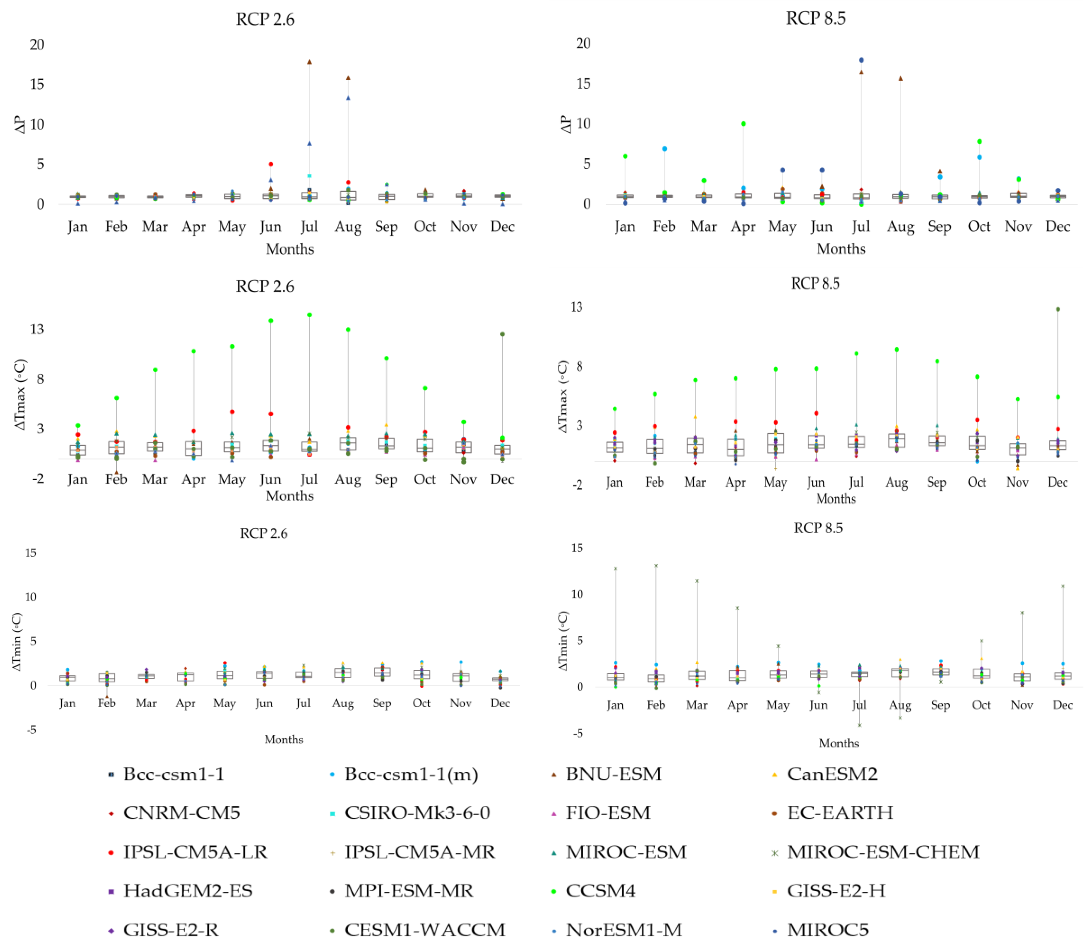
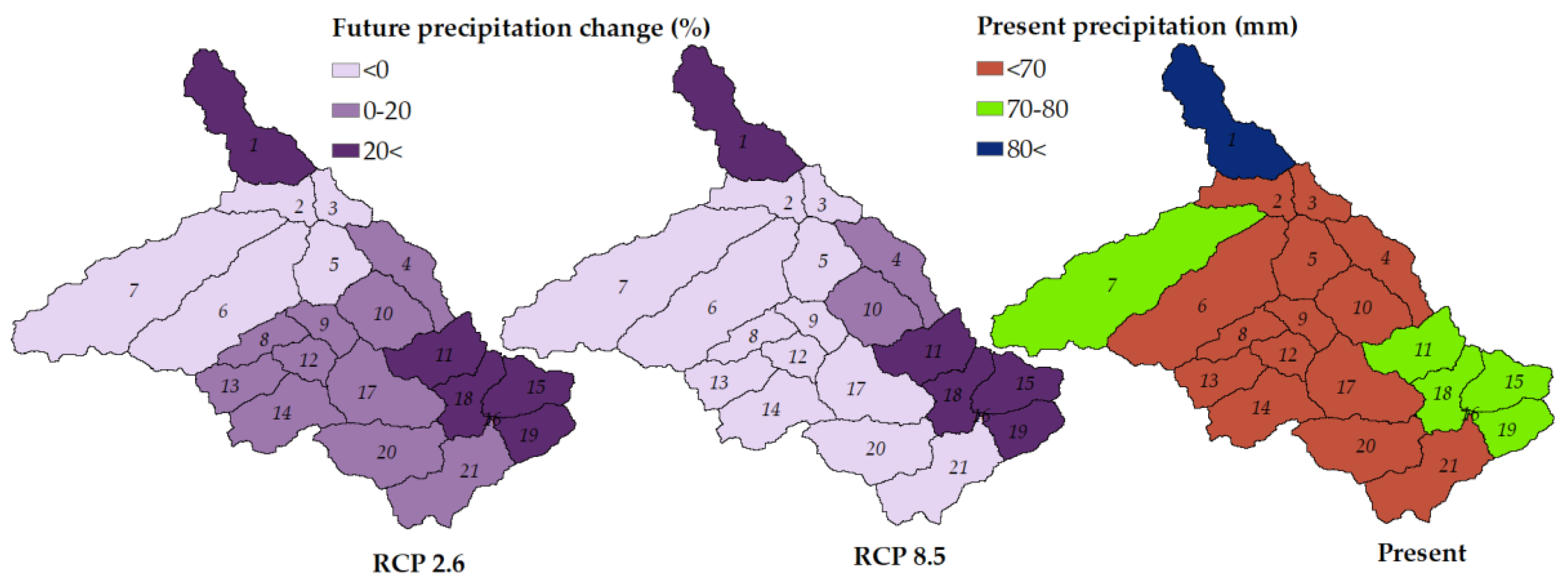
3.1. Climate Change Models and Downscaling

Variation of monthly mean precipitation and maximum and minimum temperature for the twenty CMIP5 GCMs output under RCP scenarios 2.6 and 8.5 (Figure 3) for the near future (2020–2040) relative to the present period (1984–2005) is shown as box plots in Figure 4. It is obvious that the BNU-ESM and GISS-E2-R projected more significant variation in precipitation for July and August for both RCPs. For RCP 8.5, CCSM4 and MIROC5 projected higher precipitation in April, October, and January. Precipitation variation in January, July, August, and September was largest for RCP 2.6. Results showed that variation in precipitation for all CMIP5 GCMs is quite close to the median except for July and August for both RCPs. Besides that, CCSM4 had the most substantial changes in maximum temperature for all months except December for RCP 2.6 and for all months for RCP 8.5. The CESM1-WACCM model displayed the highest changes in December for both scenarios. The results for changes in minimum temperature displayed the lowest variation for all months in RCP 2.6 that was closest to the median. The uncertainty in minimum temperature for RCP 8.5 can be seen for the MIROC-ESM-CHEM. At a glance, the projected and future changes of precipitation and maximum and minimum temperature did not show much variation between different models and quite good agreement between the CMIP5 GCMs for both RCPs near the median. Therefore, the median for all twenty CMIP5 GCMs was used to modify initial scenarios in LARS-WG (

Table 1. Median of precipitation and maximum and minimum temperature for RCP 2.6 and RCP 8.5 scenarios for each month.

Month	ΔP (2.6)	ΔP (8.5)	ΔTmax (2.6)	ΔTmax (8.5)	ΔTmin (2.6)	ΔTmin (8.5)
January	0.99	0.95	0.90	1.14	0.97	1.07
February	1.00	0.98	1.20	1.09	0.80	0.92
March	0.94	0.93	1.21	1.44	1.10	1.23
April	1.08	0.91	1.03	1.02	1.24	1.05
May	0.99	0.87	1.17	1.43	1.13	1.34
June	1.08	0.82	1.36	1.43	1.41	1.45
July	0.93	0.83	0.97	1.47	1.06	1.50
August	0.89	0.96	1.61	1.91	1.51	1.81
September	1.01	0.95	1.32	1.60	1.43	1.62
October	1.01	0.96	1.12	1.35	1.20	1.26
November	1.03	1.02	1.20	1.14	1.10	1.14
December	1.04	0.97	1.01	1.35	0.77	1.23

).

Spatial and temporal precipitation change is considered a significant input to hydrological modeling. The spatial distribution of the projected maximum precipitation for the present and near future period is shown in Figure 5. It can be seen that the most significant increase in precipitation will likely occur in the northern and southeastern part of the basin judging from both RCP scenarios. The northern and southeastern part of the basin is likely to experience a precipitation increase of more than 20% considering both RCP scenarios relative to the present period. RCP 2.6 showed an increase of about 0 to 20% from the southern toward the central parts of the basin. RCP 8.5 showed a decrease of about 0 to −10% from the southern toward central and western parts of the basin. The rest of the basin, the western and northern parts, showed a considerable decrease of precipitation for the near future for both RCPs (Figure 5).

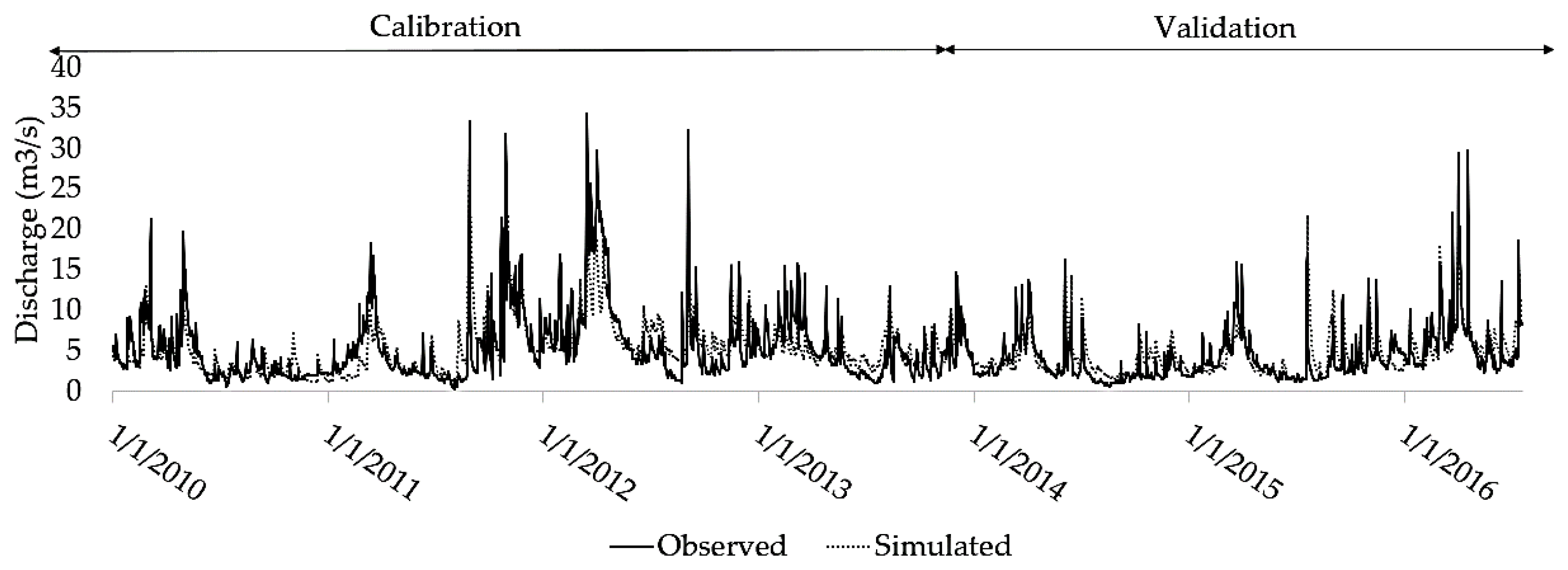
3.2. SWAT Model Calibration and Validation

Using the SUFI2 algorithm in SWAT-CUP, the sensitive parameters were adjusted to achieve the best match between observed and simulated discharge. For this, the initial values for parameter optimization, using SUFI-2 in SWAT-CUP, were acquired from literature. Then, considering the different features of the Talar River Basin including mostly climatic, topographic, and soil characteristics, the initial values were adjusted within the appropriate ranges as mentioned in SWAT documentation [47] as well as in literature. The best calibrated parameters were obtained during numerous iterations based on the achieved R² and NSE as well as model performance related to overestimation, underestimation, and the lag time between observed and simulated time series. Abbaspour et al. [51] provided some informative methods for SWAT calibration procedures in the SWAT-CUP (SUFI-2 algorithm). In this, study due to overestimation of the simulated flow, the CN2 parameter was manually adjusted upon model suggestion. In addition, SMTMP was manually adjusted to improve the performance of the model following the recommendation of Tuo et al. [65] who stated that the higher SMTMP of basin-scale parameters is related to less snowmelt. The sensitive parameters and their statistical significance are listed in

Table 2. Sensitive calibration parameter uncertainty at daily data timescale.

Rank of Parameter	Parameter	Fit	Minimum	Maximum	t-Stat	p-Value
1	V 1__SMTMP.bsn	12.92	8.47	13.05	4.67	0.00
2	A 2__GW_DELAY.gw	79.33	44.07	126.08	−2.69	0.01
3	V__RCHRG_DP.gw	0.34	0.24	0.46	1.82	0.08
4	V__CH_N2.rte	0.15	0.06	0.26	−1.53	0.14
5	R 3__CN2.mgt	−0.91	−1.25	−0.72	−1.13	0.27
6	R__ESCO.hru	0.28	0.21	0.42	0.82	0.42
7	V__CANMX.hru	34.67	27.16	46.42	−0.75	0.46
8	R__SOL_AWC(..).sol	−0.16	−0.26	−0.06	−0.70	0.49
9	R__SURLAG.bsn	3.33	−8.60	5.43	−0.70	0.49
10	V__CH_K2.rte	0.29	0.15	0.56	−0.53	0.60
11	R__SOL_Z(..).sol	0.21	0.19	0.47	−0.50	0.62
12	R__SOL_K(..).sol	0.29	−0.02	0.49	−0.40	0.69
13	V__REVAPMN.gw	107.09	89.84	113.47	0.36	0.72
14	V__GWQMN.gw	4336.60	4253.70	4806.40	0.28	0.78
15	R__SOL_ALB(..).sol	0.02	−0.10	0.03	−0.22	0.83
16	V__ALPHA_BF.gw	0.30	0.06	0.35	0.17	0.86
17	R__SOL_BD(..).sol	−0.26	−0.31	−0.15	0.15	0.88
18	R__GWHT.gw	0.07	−0.19	0.19	0.11	0.91

¹ V is the existing parameter value to be replaced by a given value. ² A is the given value added to the existing parameter value. ³ R is the existing parameter value × (1 + a given value) [45].

.

Acceptable range and fitted values based on the Nash–Sutcliffe, Coefficient of Determination, and other algorithms are embedded in the SWAT-CUP [66]. Through about 2000 iterations in each simulation, the SWAT-CUP determined the best fit using the most sensitive parameters (Table 2).

The t-stat and p-value were used to quantify the sensitivity and relative significance of each parameter (Table 2). Eighteen parameters were detected as sensitive parameters and consequently ranked.

Generally, the threshold depth of water in the shallow aquifer (REVAPMN), base flow alpha factor (ALPHA_BF), threshold depth of water in the shallow aquifer required for return flow (GWQMN), deep aquifer percolation fraction (RCHRG_DP), initial groundwater height (GWHT), groundwater delay (GW_DELAY), and deep aquifer percolation fraction (RCHRG_DP) are related to groundwater information. Available water capacity of the soil layer (SOL_AWC), moist bulk density (SOL_BD), moist soil albedo (SOL_ALB), depth from the soil surface to bottom layer (SOL_Z), and saturated hydraulic conductivity (SOL_K) refer to soil parameters. Soil evaporation compensation factor (ESCO) and maximum canopy storage (CANMX) refer to evaporation. Snowmelt base temperature (SMTMP) and surface runoff lag time (SURLAG) are sensitive parameters governing the basin response. Manning’s “n” for the main channel (CH_N2) and effective hydraulic conductivity in main channel alluvium (CH_K2) are main channel sensitive parameters and the initial SCS runoff curve number to moisture condition II (CN2) is considered as a management parameter [67]. Consequently, SMTMP, GW_DELAY, RCHRG_DP, CH_N2 and CN2 were ranked as the most sensitive parameters in the modeling procedure (based on p-value and t-stat) and hence, played essential roles in the calibration and validation of the SWAT model (Table 2).

Based on generally acceptable performance criteria [68,69], the SWAT model was well calibrated (R² = 0.67 and NSE = 0.61) and validated (R² = 0.58 and NSE = 0.55). The performance outcomes represent uncertainty in the model and are probably related to significant variation in topography and rainfall [70].

Simulated daily discharge matched the observed for the calibration and validation periods with R² = 0.67 and 0.58 and NSE = 0.61 and 0.55, respectively. Consequently, it may be said that the simulated and observed discharge showed good agreement for the calibration and validation periods (Figure 6).

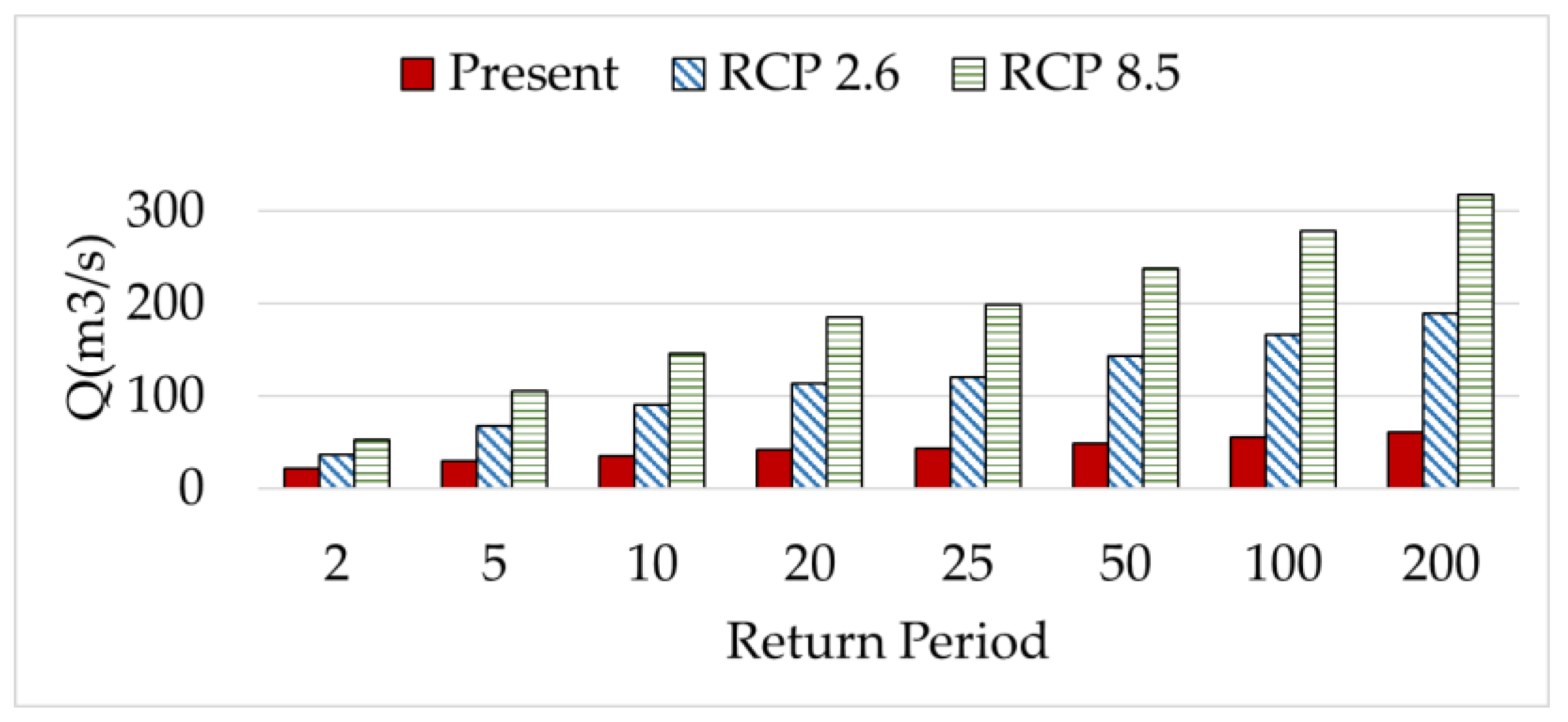
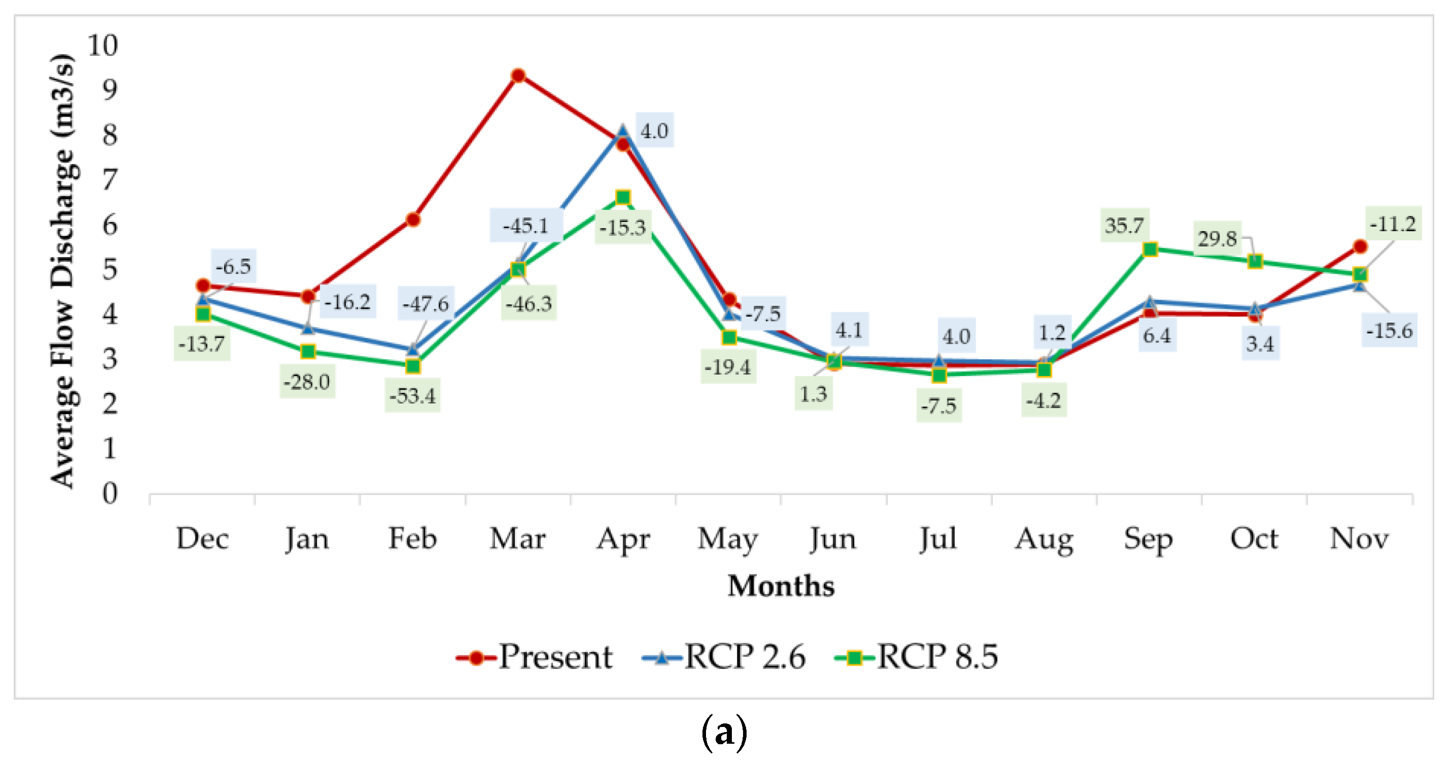
3.3. Analysis of Flood Frequency

The best method for IPF estimation was selected based on the R², NSE, RMSE, and MAE criterion. Comparison between observed and estimated IPF by the four empirical methods for the present period (

Table 3. Statistical comparison of Fuller, Sangal, Fill–Steiner, and Slope-based methods for the present period.

Index	Sangal	Fill–Steiner	Fuller	Slope-Based
R2	0.76	0.78	0.80	0.74
NSE	0.48	0.48	0.90	0.36
RMSE (m3 s−1)	19.68	19.69	19.09	21.77
MAE (m3 s−1)	4.77	9.67	8.9	9.8

) showed that the Fuller method is a more accurate technique (R² = 0.8 and NSE = 0.9). Consequently, the Fuller method was selected for IPF based estimation for future flood assessment. The generated precipitation and temperature from the previous section were fed into the SWAT model to generate a future daily discharge. In this regard, the selected method for IPF (Fuller), was used to estimate the IPF in the future, as well.

The effect of the two RCPs on peak discharge at the main outlet was investigated with different return periods from 2 to 200 years (Figure 7). It can be seen that the flood amount increases for RCP 8.5 and RCP 2.6 in comparison to the present period. These results are consistent with the study carried out by Abbaspour et al. [13], who showed that the northern parts of Iran will likely experience larger and more intense flooding events in the future. However, Almasi and Soltani [24] concluded that the IPF and flood magnitude are likely to decrease in the near future, considering two emission scenarios (A1 and B1) of the GCMs of IPCC’s fourth assessment report (AR4) for the Bazoft River Basin. Khazaei et al. [71] showed that climate change is likely to increase flood events in the Pataveh River Basin. Therefore, different studies show different results depending on geographic location in Iran. A probable explanation for these differences is that flood impact not only depends on projected climate change but also on slope, change in agricultural area use, and urban influence.

Figure 8 shows the average discharge at the outlet of the Talar River Basin estimated by the SWAT model for the present and near future scenarios. As can be observed, there are slight differences between the outflow using RCP 2.6 and 8.5 scenarios from June to August. The average monthly flow (Figure 8a) shows a decrease relative to the present flow conditions in February and March by −48% and −45% for RCP 2.6, respectively, and −53% and −46% for RCP 8.5, respectively. Increase in September (36%) and October (30%) can be seen for RCP 8.5 (Figure 8a). The average seasonal discharge at the outlet of the main basin is depicted in Figure 8b. According to the figure, there is a more significant change between the present and the near future simulated flow. The discharge pattern shows that the highest decrease will likely occur in winter by −34% in the case of RCP 8.5 and by −26% for RCP 2.6 and a considerable decrease during spring season mainly due to a decrease in March. The summer season does not reveal a big change for the future scenarios. Figure 9 shows the monthly maximum IPF estimation for the main outlet. It can be seen that maximum IPF is projected in September and November for both RCP scenarios that can be explained by the different precipitation pattern and climate change model selection. In addition, the reduction of streamflow can be due to the agricultural use in this area.

3.4. Subbasin Instantaneous Peak Flow (IPF) Estimation

Figure 10 shows the distribution of change for maximum IPF over the Talar River Basin for the present and near future. Maximum IPF during the present period is mainly observed in the downstream area, which includes Subbasina number 1, 3, and 5 by more than 30 m³ s⁻¹ and Subbasin 10 and 17 by 10–30 m³ s⁻¹ for the main river in the basin. Figure 10 shows the per cent change of IPF for RCP 2.6 and 8.5. The largest increase of IPF will likely occur in subbasins that are located near the vicinity of the main outlet (Subbasins 1, 2, 6, and 4) for RCP 2.6. As IPF values are highly sensitive to increase in maximum rainfall, it can be seen, e.g., that increase of maximum rainfall (more than 20% for both RCPs in the southeastern regions covering Subbasins 11, 18, 15, and 19) caused an increase of IPF in the downstream Subbasin 4.

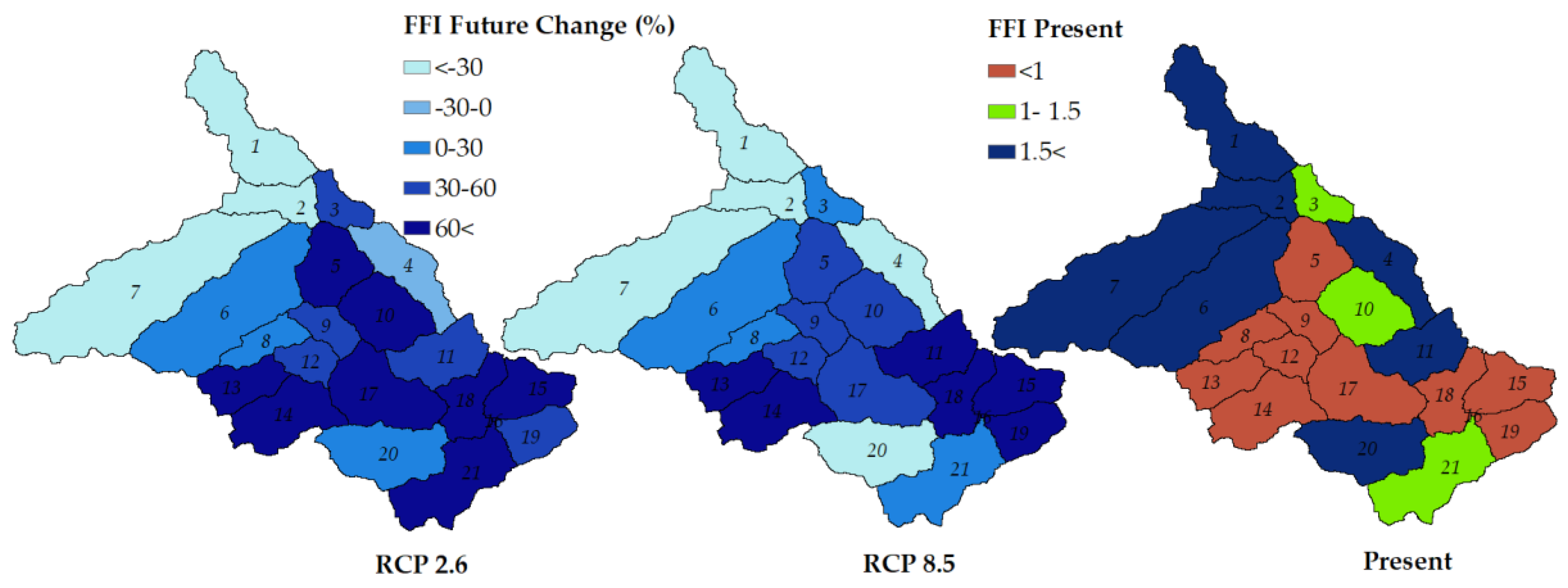
3.5. Flood Frequency Index (FFI)

Figure 11 illustrates the spatial distribution of Flood Frequency Index (FFI) for the present period and percent change in the near future. According to the figure, Subbasins 1, 2, 6, 7, 4, 11, and 20 show a greater FFI as compared to other subbasins for the present period. The comparably high FFI may be because these subbasins are highly populated and the majority of the land is urbanized rather than other subbasins. In principle, the flood risk in the northern, i.e., Subbasins 1, 2, 6, 7, and 4 are higher than other parts of the basin for the present period. This is probably related to the high urbanization rate and deforestation for expanding agricultural land in this region.

The percent change of FFI will likely increase by more than 60% relative to the present period in the eastern parts considering both RCPs. The per cent change of FFI will likely decrease relative to the present period in northern subbasins, i.e., 1, 2, 7, and 4, for both RCPs.

It can be seen that the central parts that have the lowest FFI in the present climate (<1) will likely increase in the future. On the contrary, the northern region that has higher FFI will likely experience a decrease or slight increase in the future.

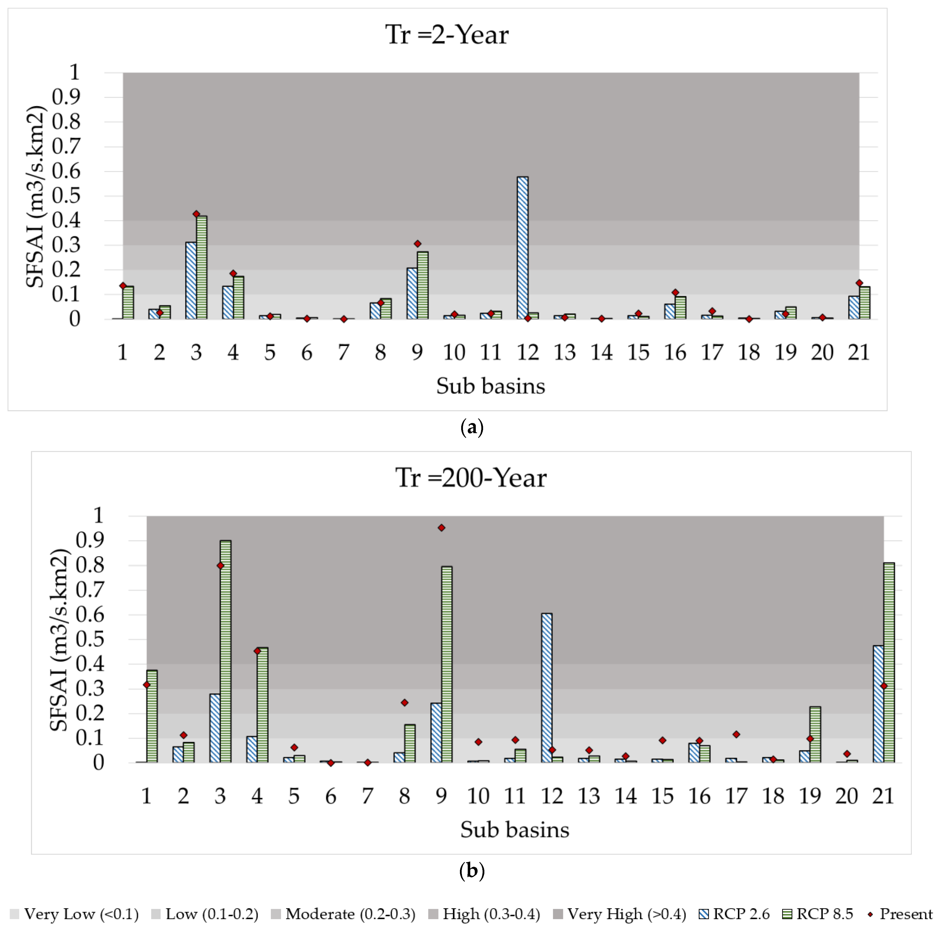
3.6. Subbasin Flood Source Area Index (SFSAI)

Figure 12 shows the results of the Subbasin Flood Source Area Index (SFSAI) according to the SFSAI classification including very low (<0.1), low (0.1–0.2), moderate (0.2–0.3), high (0.3–0.4), and very high (>0.4) for different return periods (2 to 200 years). This classification approach was used to rank the subbasins with regard to their contribution to flood generation at the main outlet of the studied basin for the present and near future period. According to these results, for a 2-year return period, Subbasins 3, 9, and 4 show very high, high, and moderate SFSAI for the present climate. In other words, these subbasins and their upstream subbasins have the largest effect on the main outflow discharge. For example, Subbasin 3 has the highest SFSAI for the present period, 0.41 and 0.8 for 2- and 200-year return period, respectively. This indicates a major contribution of Subbasins 4, 5, and 10, to the recorded discharge at the Talar Basin’s outlet. Subbasin 12, 3, and 9 indicated very high, high, and moderate SFSAI for RCP 2.6, which shows that more significant floods relative to the present period can be expected in the near future. For Subbasin 12, the SFSAI changed from very low (0.02) to very high (0.6), and in Subbasin 3, SFSAI changed from very high (0.41) to high (0.31) for RCP 2.6 and a 2-year return period. Based on RCP 2.6, Subbasin 12 indicates an increase from very low at present to very high SFSAI in the near future. This means that this area could be expected to face a major flood event in the near future considering RCP 2.6. Based on our findings, high flood source subbasins are mostly located in the central and northeastern parts of the Talar Basin, which are characterized by high mountains and urban areas.

4. Summary and Conclusions

This study addressed the temporal and spatial impact of climate change on flood frequency and source area in subbasins of the Talar River Basin in northern Iran under low and high RCP scenarios (2.6 and 8.5). For this purpose, the model was firstly calibrated and validated during the 2010–2013 and 2014–2016 periods, respectively, at a daily time scale. Then, the future projected climate variables (precipitation and maximum and minimum temperature) from CMIP5 GCM models were downscaled in LARS-WG and fed into the Soil and Water Assessment Tool (SWAT) to investigate the potential impact of climate change on the flood properties. The SWAT model has previously been applied for monthly simulation of flow in the studied basin [27]. However, in this study we calibrated and validated the model at a daily time step using a large range of input parameters. Results show that the agreement between observed and simulated daily discharge is acceptable and that the calibrated SWAT can be used to evaluate the flood response to climate change. Further, in this study we also applied future climate scenarios and assessed flood properties in the near future using a calibrated SWAT model. For the climate change modeling, an ensemble of twenty CMIP5 GCMs based on IPCC Fifth Assessment Report under two climate change scenarios (2.6 and 8.5) was used. The period 2020–2040 was selected as near future period for the analysis. Four IPF estimation methods were tested for the present period and the best method, the Fuller method, was chosen as it showed the best agreement between observed and estimated IPF for the present period. The empirical method was then used for the near future IPF estimation. To project the flood condition in the near future for the studied basin, Flood Frequency Index (FFI) and Sub Basin Flood Source Area (SFSA) were applied.

Regarding the CMIP5 GCMs uncertainty, the BNU-ESM model showed a maximum increase of precipitation for both RCPs during July and August and the CCSM4 in projecting maximum temperature. The MICRO-ESM-CHEM showed a higher decrease of minimum temperature projected for July, August, June, and September, respectively, and a higher increase for the remaining months. Generally, the median for all twenty CMIP5 GCMs showed an increasing range of precipitation from 0.9 to 1.08 and 0.82 to 1.02 for RCP 2.6 and 8.5, respectively. For maximum temperature, values ranged from 0.9 to 1.6 and 1.01 to 1.91 for RCP 2.6 and 8.5, respectively. Minimum temperature ranged from 0.77 to 1.50 and 0.92 to 1.8 for RCP 2.6 and 8.5, respectively. Therefore, the range of uncertainty in precipitation and temperature is not expected to change much and only slightly increase as time progresses. These results regarding future projected temperature and precipitation are similar to studies conducted for the Neka River [72] and Darab Kola Forest [73] in the vicinity of our study basin.

Another study that assessed the impact of future climate change on stream flow in Gorganroud Basin in northern Iran, found a major increase in maximum temperature in May and June and minor increase in April and November. They also suggested a major increase for minimum temperature in August, September, and May and a minor increase in November. Further, that study concluded that climate change impact on streamflow in the future will likely result in a different temporal pattern relative to the present period at monthly scale depending on the individual model scenarios [74]. Although their results are slightly different compared to the present study, both studies confirm an increase in temperature, precipitation, and streamflow for river basins in the north of Iran.

Results revealed that the projected climate change impact could lead to an average discharge decrease in February, March, and January for both RCPs and increase in September and October for RCP 8.5. The maximum and minimum temperature will likely increase for all months in the near future. In principle, the annual precipitation could increase by more than 20% in the near future, which can be translated into an increase of IPF. Also, the flood frequency pattern for the present period showed that the southern and central parts of the basin have the lowest FFI (<1). This means that almost no change may occur from now to the near future. The eastern parts displayed an increase of FFI for both RCPs.

Results showed that in most subbasins, the RCP 8.5 displays higher SFSA rather than RCP 2.6. Subbasins 3 and 9 could be crucial subbasins due to the fact that they represent the most significant contribution to the total peak discharge at the basin outlet for the present and near future. The flood source area results indicate that SFSA will likely increase to very high in Subbasins 12 for RCP 2.6. Subbasins 3 and 9 for both RCP scenarios showed a higher rank for SFSA as compared to the present period.

The findings are useful for flood management considering the various sources of runoff in the upstream area rather than just taking into account the downstream flood-threatened areas. The results can be used to find the best location for establishing real-time flood forecasting and warning systems. However, the performance of the considered twenty CMIP5 GCMs did not show a high variation in projected precipitation and maximum and minimum temperature. We did not investigate uncertainties related to climate model outputs. Hence, downscaling approaches should be investigated in future studies. Future studies could investigate SWAT modeling for assessment of uncertainty using this model. Previous studies have reported that land use change can significantly affect the flood peak generation and flood source area [64]. Since previous studies in this basin have shown that effects of land use change on water flow and nitrate loads are significant [27], it is suggested that the effect of land use options on flood source area and flood frequency pattern in Talar River Basin can be investigated in further studies. Management practices can be applied using the calibrated model to understand their effect on reducing flood source area. It should be noted that the results of this study are important for water managers and policymakers to define mitigation and adaptation strategies in the Talar and similar river basins.

References

1. Asgharpour, S.E.; Ajdari, B. A case study on seasonal floods in Iran, watershed of Ghotour Chai Basin. Procedia Soc. Behav. Sci. 2011, 19, 556–566. [Google Scholar] [CrossRef]
2. The Core Writing Team; Pachauri, R.K.; Meyer, L. (Eds.) Climate Change 2014: Synthesis Report. Contribution of Working Groups I, II and III to the Fifth Assessment Report of the Intergovernmental Panel on Climate Change; IPCC: Geneva, Switzerland, 2014; p. 151. [Google Scholar] [CrossRef]
3. Duan, J.G.; Bai, Y.; Dominguez, F.; Rivera, E.; Meixner, T. Framework for incorporating climate change on flood magnitude and frequency analysis in the upper Santa Cruz River. J. Hydrol. 2017, 549, 194–207. [Google Scholar] [CrossRef]
4. Reynard, N.; Crooks, S.; Wilby, R.; Kay, A. Climate change and flood frequency in the UK. In Proceedings of the 39th Defra Flood and Coastal Flood Management Conference, York, UK, 29 June–1 July 2004; pp. 1–12. [Google Scholar]
5. Amiri, M.J.; Eslamian, S.S. Investigation of climate change in Iran. J. Environ. Sci. Technol. 2010, 3, 208–216. [Google Scholar] [CrossRef]
6. Das, S.; Simonovic, S.P. Assessment of Uncertainty in Flood Flows under Climate Change: The Upper Thames River Basin (Ontario, Canada); University of Western Ontario: London, ON, Canada, 2012. [Google Scholar]
7. Mallakpour, I.; Villarini, G. The changing nature of flooding across the central United States. Nat. Clim. Chang. 2015, 5, 250–254. [Google Scholar] [CrossRef]
8. Alfieri, L.; Burek, P.; Feyen, L.; Forzieri, G. Global warming increases the frequency of river floods in Europe. Hydrol. Earth Syst. Sci. 2015, 19, 2247–2260. [Google Scholar] [CrossRef]
9. Krysanova, V.; Vetter, T.; Eisner, S.; Huang, S.; Pechlivanidis, I.; Strauch, M.; Gelfan, A.; Kumar, R.; Aich, V.; Arheimer, B.; et al. Intercomparison of regional-scale hydrological models and climate change impacts projected for 12 large river basins worldwide—A synthesis. Environ. Res. Lett. 2017, 12, 105002. [Google Scholar] [CrossRef]
10. Hashemi, H. Climate change and the future of water management in Iran. Middle East Crit. 2015, 24, 307–323. [Google Scholar] [CrossRef]
11. Hashemi, H.; Uvo, C.B.; Berndtsson, R. Coupled modeling approach to assess climate change impacts on groundwater recharge and adaptation in arid areas. Hydrol. Earth Syst. Sci. 2015, 19, 4165–4181. [Google Scholar] [CrossRef]
12. Welde, K. Identification and prioritization of subwatersheds for land and water management in Tekeze dam watershed, Northern Ethiopia. Int. Soil Water Conserv. Res. 2016, 4, 30–38. [Google Scholar] [CrossRef]
13. Abbaspour, K.C.; Faramarzi, M.; Ghasemi, S.S.; Yang, H. Assessing the impact of climate change on water resources in Iran. Water Resour. Res. 2009, 45. [Google Scholar] [CrossRef]
14. Covey, C.; AchutaRao, K.M.; Cubasch, U.; Jones, P.; Lambert, S.J.; Mann, M.E.; Phillips, T.J.; Taylor, K.E. An overview of results from the Coupled Model Intercomparison Project. Glob. Planet. Chang. 2003, 37, 103–133. [Google Scholar] [CrossRef]
15. Miao, C.; Duan, Q.; Sun, Q.; Huang, Y.; Kong, D.; Yang, T.; Ye, A.; Di, Z.; Gong, W. Assessment of CMIP5 climate models and projected temperature changes over Northern Eurasia. Environ. Res. Lett. 2014, 9, 055007. [Google Scholar] [CrossRef]
16. Moss, R.H.; Edmonds, J.A.; Hibbard, K.A.; Manning, M.R.; Rose, S.K.; Van Vuuren, D.P.; Carter, T.R.; Emori, S.; Kainuma, M.; Kram, T.; et al. The next generation of scenarios for climate change research and assessment. Nature 2010, 463, 747–756. [Google Scholar] [CrossRef] [PubMed]
17. Quintero, F.; Mantilla, R.; Anderson, C.; Claman, D.; Krajewski, W. Assessment of Changes in Flood Frequency Due to the Effects of Climate Change: Implications for Engineering Design. Hydrology 2018, 5, 19. [Google Scholar] [CrossRef]
18. Pitta, S.K. A case study on flood frequency analysis. Int. J. Civ. Eng. Technol. 2017, 8, 1762–1767. [Google Scholar]
19. Argaw, Y. Flood Frequency Analysis for Lower Awash Subbasin (Tributaries from Northern Wollo High Lands) Using SWAT 2005 Model. Master’s Thesis, Addis Ababa University, Addis Ababa, Ethiopia, 2008. [Google Scholar]
20. Saghafian, B.; Golian, S.; Elmi, M.; Akhtari, R. Monte Carlo analysis of the effect of spatial distribution of storms on prioritization of flood source areas. Nat. Hazards 2013, 66, 1059–1071. [Google Scholar] [CrossRef]
21. Huang, X.; Wang, L.; Han, P.; Wang, W. Spatial and Temporal Patterns in Nonstationary Flood Frequency across a Forest Watershed: Linkage with Rainfall and Land Use Types. Forests 2018, 9, 339. [Google Scholar] [CrossRef]
22. Saghafian, B.; Ghermezcheshmeh, B.; Kheirkhah, M.M. Iso-flood severity mapping: A new tool for distributed flood source identification. Nat. Hazards 2010, 55, 557–570. [Google Scholar] [CrossRef]
23. Camici, S.; Brocca, L.; Melone, F.; Moramarco, T. Impact of climate change on flood frequency using different climate models and downscaling approaches. J. Hydrol. Eng. 2014, 19, 04014002. [Google Scholar] [CrossRef]
24. Almasi, P.; Soltani, S. Assessment of the climate change impacts on flood frequency (case study: Bazoft Basin, Iran). Stoch. Environ. Res. Risk Assess. 2016, 31, 1171–1182. [Google Scholar] [CrossRef]
25. Prudhomme, C.; Jakob, D.; Svensson, C. Uncertainty and climate change impact on the flood regime of small UK catchments. J. Hydrol. 2003, 277, 1–23. [Google Scholar] [CrossRef]
26. Gholami, V.; Khaleghi, M.; Zabardast Rostami, H. Hydrological impacts of Chashm dam on the downstream of Talar River Watershed, Iran. Int. J. Agric. Res. Crop Sci. 2017, 1, 9–20. [Google Scholar]
27. Kavian, A.; Mohammadi, M.; Gholami, L.; Rodrigo-Comino, J. Assessment of the spatiotemporal effects of land use changes on runoff and nitrate loads in the Talar River. Water 2018, 10, 445. [Google Scholar] [CrossRef]
28. Zare, M.; Panagopoulos, T.; Loures, L. Simulating the impacts of future land use change on soil erosion in the Kasilian Watershed, Iran. Land Use Policy 2017, 67, 558–572. [Google Scholar] [CrossRef]
29. Jahanshahi, A.; Golshan, M.; Afzali, A. Simulation of the catchments hydrological processes in arid, semi-arid and semi-humid areas. Desert 2017, 22, 1–10. [Google Scholar]
30. Azmoodeh, A.; Kavian, A.; Habib Nejad Roshan, M.; Zeinivand, H.; Goudarzi, M. Forecasting of land use changes based on land change modeler (LCM) using remote sensing: A case study of Talar Watershed, Mazandaran province, northern Iran. Adv. Biores. 2016, 8, 22–32. [Google Scholar] [CrossRef]
31. Jahad Engineering Services Company. Comprehensive Studies of Talar Watershed; Office of Watershed Studies Evaluation: Sari, Mazandaran, Iran, 2001. [Google Scholar]
32. Lutz, A.F.; ter Maat, H.W.; Biemans, H.; Shrestha, A.B.; Wester, P.; Immerzeel, W.W. Selecting representative climate models for climate change impact studies: An advanced envelope-based selection approach. Int. J. Climatol. 2016, 36, 3988–4005. [Google Scholar] [CrossRef]
33. Shrestha, S.; Shrestha, M.; Babel, M.S. Modelling the potential impacts of climate change on hydrology and water resources in the Indrawati River Basin, Nepal. Environ. Earth Sci. 2016, 75, 280. [Google Scholar] [CrossRef]
34. Tian, Y.; Xu, Y.-P.; Booij, M.J.; Cao, L. Impact assessment of multiple uncertainty sources on high flows under climate change. Hydrol. Res. 2015, 47, 61–74. [Google Scholar] [CrossRef]
35. Buser, C.M.; Kunsch, H.R.; Luthi, D.; Wild, M.; Schar, C. Bayesian multi-model projection of climate: Bias assumptions and interannual variability. Clim. Dyn. 2009, 33, 849–868. [Google Scholar] [CrossRef]
36. Knutti, R.; Sedláček, J. Robustness and uncertainties in the new CMIP5 climate model projections. Nat. Clim. Chang. 2013, 3, 369–373. [Google Scholar] [CrossRef]
37. Semenov, M.A.; Barrow, E.M. LARS-WG: A Stochastic Weather Generator for Use in Climate Impact Studies; User Manual; Rothamsted Research: Hertfordshire, UK, 2002; pp. 1–27. [Google Scholar]
38. Semenov, M.A. Simulation of extreme weather events by a stochastic weather generator. Clim. Res. 2008, 35, 203–212. [Google Scholar] [CrossRef]
39. Semenov, M.A.; Stratonovitch, P. Use of multi-model ensembles from global climate models for assessment of climate change impacts. Clim. Res. 2010, 41, 1–14. [Google Scholar] [CrossRef]
40. Vaighan, A.A.; Talebbeydokhti, N.; Bavani, A.M. Assessing the impacts of climate and land use change on streamflow, water quality and suspended sediment in the Kor River Basin, Southwest of Iran. Environ. Earth Sci. 2017, 76, 543. [Google Scholar] [CrossRef]
41. Praskievicz, S.; Chang, H. A review of hydrological modelling of basin-scale climate change and urban development impacts. Prog. Phys. Geogr. 2009, 33, 650–671. [Google Scholar] [CrossRef]
42. Amengual, A.; Romero, R.; Gómez, M.; Martín, A.; Alonso, S. A hydrometeorological modeling study of a flash-flood event over Catalonia, Spain. J. Hydrometeorol. 2006, 8, 282–303. [Google Scholar] [CrossRef]
43. Mehan, S.; Neupane, R.P.; Kumar, S. Coupling of SUFI 2 and SWAT for improving the simulation of streamflow in an agricultural watershed of South Dakota. Hydrol. Curr. Res. 2017, 8, 3. [Google Scholar] [CrossRef]
44. Arnold, J.G.; Srinivasan, R.; Muttiah, R.S.; Williams, J.R. Large area hydrologic modeling and assessment Part I: Model development. J. Am. Water Resour. Assoc. 1998, 34, 73–89. [Google Scholar] [CrossRef]
45. Abbaspour, K.C. SWAT-CUP: SWAT Calibration and Uncertainty Programs—A User Manual; Eawag: Dübendorf, Switzerland, 2015. [Google Scholar] [CrossRef]
46. Kiros, G.; Shetty, A.; Nandagiri, L. Performance evaluation of SWAT model for land use and land cover changes under different climatic conditions: A review. Hydrol. Curr. Res. 2015, 6, 3. [Google Scholar] [CrossRef]
47. Neitsch, S.L.; Arnold, J.G.; Kiniry, J.R.; Williams, J.R. Soil & Water Assessment Tool Theoretical Documentation Version 2009; Texas Water Resources Institute Technical Report: College Station, TX, USA, 2011; pp. 1–647. [Google Scholar] [CrossRef]
48. Faramarzi, M.; Abbaspour, K.C.; Schulin, R.; Yang, H. Modelling blue and green water resources availability in Iran. Hydrol. Process. 2009, 23, 486–501. [Google Scholar] [CrossRef]
49. Xu, X.; Wang, Y.C.; Kalcic, M.; Muenich, R.L.; Yang, Y.C.E.; Scavia, D. Evaluating the impact of climate change on fluvial flood risk in a mixed-used watershed. Environ. Model. Softw. 2017. [Google Scholar] [CrossRef]
50. Goyal, M.K.; Panchariya, V.K.; Sharma, A.; Singh, V. Comparative assessment of SWAT model performance in two distinct catchments under various DEM scenarios of varying resolution, sources and resampling methods. Water Resour. Manag. 2018, 32, 805–825. [Google Scholar] [CrossRef]
51. Abbaspour, K.C.; Rouholahnejad, E.; Vaghefi, S.; Srinivasan, R.; Yang, H.; Kløve, B. A continental-scale hydrology and water quality model for Europe: Calibration and uncertainty of a high-resolution large-scale SWAT model. J. Hydrol. 2015, 524, 733–752. [Google Scholar] [CrossRef]
52. Bajracharya, A.R.; Bajracharya, S.R.; Shrestha, A.B.; Maharjan, S.B. Climate change impact assessment on the hydrological regime of the Kaligandaki Basin, Nepal. Sci. Total Environ. 2018, 625, 837–848. [Google Scholar] [CrossRef] [PubMed]
53. Me, W.; Abell, J.M.; Hamilton, D.P. Effects of hydrologic conditions on SWAT model performance and parameter sensitivity for a small, mixed land use catchment in New Zealand. Hydrol. Earth Syst. Sci. 2015, 19, 4127–4147. [Google Scholar] [CrossRef]
54. Srinivas, G.; Gopal, M.N. Hydrological modeling of Musi River Basin, India and sensitive parameterization of streamflow using SWAT CUP. J. Hydrogeol. Hydrol. Eng. 2017, 6, 2–11. [Google Scholar] [CrossRef]
55. Yang, J.; Reichert, P.; Abbaspour, K.C.; Xia, J.; Yang, H. Comparing uncertainty analysis techniques for a SWAT application to the Chaohe Basin in China. J. Hydrol. 2008, 358, 1–23. [Google Scholar] [CrossRef]
56. Moriasi, D.N.; Arnold, J.G.; Van Liew, M.W.; Bingner, R.L.; Harmel, R.D.; Veith, T.L. Model evaluation guidelines for systematic quantification of accuracy in watershed simulations. Trans. ASABE 2007, 50, 885–900. [Google Scholar] [CrossRef]
57. Dibike, Y.B.; Coulibaly, P. Downscaling of Global Climate Model Outputs for Flood Frequency Analysis in the Saguenay River System; Department of Civil Engineering/School of Geography and Geology, McMaster University: Hamilton, ON, Canada, 2004. [Google Scholar]
58. Chen, B.; Krajewski, W.F.; Liu, F.; Fang, W.; Xu, Z. Estimating instantaneous peak flow from mean daily flow. Hydrol. Res. 2017. [Google Scholar] [CrossRef]
59. Fuller, W.E. Flood flows. Trans. Am. Soc. Civ. Eng. 1914, 77, 564–617. [Google Scholar]
60. Sangal, B.P. Practical method of estimating peak flow. J. Hydraul. Eng. 1983, 109, 549–563. [Google Scholar] [CrossRef]
61. Saghafian, B.; Khosroshahi, M. Unit response approach for priority determination of flood source areas. J. Hydrol. Eng. 2005, 10, 23–38. [Google Scholar] [CrossRef]
62. Gharib, M.; Motamedvaziri, B.; Ghermezcheshmeh, B.; Ahmadi, H. Evaluation of ModClark model for simulating rainfall-runoff in Tangrah Watershed, Iran. Appl. Ecol. Environ. Res. 2018, 16, 1053–1068. [Google Scholar] [CrossRef]
63. Suriya, S.; Mudgal, B.V. Assessment of flood potential ranking of subwatersheds: Adayar Watershed a case study. Int. J. Innov. Res. Sci. Eng. Technol. 2014, 3, 14537–14548. [Google Scholar]
64. Saghafian, B.; Farazjoo, H.; Bozorgy, B.; Yazdandoost, F. Flood intensification due to changes in land use. Water Resour. Manag. 2008, 22, 1051–1067. [Google Scholar] [CrossRef]
65. Tuo, Y.; Marcolini, G.; Disse, M.; Chiogna, G. Calibration of snow parameters in SWAT: Comparison of three approaches in the Upper Adige River basin (Italy). Hydrol. Sci. J. 2018, 63, 657–678. [Google Scholar] [CrossRef]
66. Vilaysane, B.; Takara, K.; Luo, P.; Akkharath, I.; Duan, W. Hydrological stream flow modelling for calibration and uncertainty analysis using SWAT model in the Xedone River Basin, Lao PDR. Procedia Environ. Sci. 2015, 28, 380–390. [Google Scholar] [CrossRef]
67. Neitsch, S.L.; Arnold, J.G.; Kiniry, J.R.; Srinivasan, R.; Williams, J.R. Soil and Water Assessment Tool User’s Manual, Version 2000; Texas Water Resources Institute: College Station, TX, USA, 2002; p. 412. [Google Scholar]
68. Moriasi, D.N.; Gitau, M.W.; Pai, N.; Daggupati, P. Hydrologic and Water Quality Models: Performance Measures and Evaluation Criteria. Trans. ASABE 2015, 58, 1763–1785. [Google Scholar] [CrossRef]
69. Boithias, L.; Sauvage, S.; Lenica, A.; Roux, H.; Abbaspour, K.C.; Larnier, K.; Dartus, D.; Sánchez-Pérez, J.M. Simulating flash floods at hourly time-step using the SWAT model. Water 2017, 9, 929. [Google Scholar] [CrossRef]
70. Tejaswini, V.; Sathian, K.K. Calibration and validation of SWAT model for Kunthipuzha Basin using SUFI-2 algorithm. Int. J. Curr. Microbiol. Appl. Sci. 2018, 7, 2162–2172. [Google Scholar] [CrossRef]
71. Khazaei, M.R.; Zahabiyoun, B.; Saghafian, B. Assessment of climate change impact on floods using weather generator and continuous rainfall-runoff model. Int. J. Climatol. 2012, 32, 1997–2006. [Google Scholar] [CrossRef]
72. Joorabian Shooshtari, S.; Shayesteh, K.; Gholamalifard, M.; Azari, M.; Serrano-Notivoli, R.; López-Moreno, J.I. Impacts of future land cover and climate change on the water balance in northern Iran. Hydrol. Sci. J. 2017, 62, 2655–2673. [Google Scholar] [CrossRef]
73. Soleimani, A.; Mohsen, S.; Reza, A.; Bavani, M.; Jafari, M.; Francaviglia, R. Simulating soil organic carbon stock as affected by land cover change and climate change, Hyrcanian forests (northern Iran). Sci. Total Environ. 2017, 599–600, 1646–1657. [Google Scholar] [CrossRef] [PubMed]
74. Azari, M.; Moradi, H.R.; Saghafian, B. Climate change impacts on streamflow and sediment yield in the North of Iran. Hydrol. Sci. J. 2016, 61, 123–133. [Google Scholar] [CrossRef]
Figure 1. (a) Location of the Talar River Basin in northern Iran, (b) temperature, rainfall and discharge stations, and stream network.
Water 11 00273 g001
Figure 2. (a) Land use and (b) slope (%) of the Talar River Basin.
Water 11 00273 g002aWater 11 00273 g002b
Figure 3. Schematic of applied methodology in this study.
Water 11 00273 g003
Figure 4. Variation of monthly mean precipitation and maximum and minimum temperature for twenty CMIP5 GCMs using RCP 2.6 and RCP 8.5. The lower end of the bar represents the 5th percentile, the upper end represents the 95th percentile, and the gray box represents the 50th percentile.
Water 11 00273 g004
Figure 5. Spatial precipitation pattern at present and precipitation change in percent in the near future (RCP 2.6 and RCP 8.5).
Water 11 00273 g005
Figure 6. Comparison between observed and simulated streamflow during the calibration and validation periods.
Water 11 00273 g006
Figure 7. Discharge at the main outlet of the studied basin for 2- to 200-year return period for the present and near future based on the estimated IPF (m3 s−1) using the Fuller method.
Water 11 00273 g007
Figure 8. (a) Monthly and (b) seasonal average discharge simulation for present and near future periods.
Water 11 00273 g008aWater 11 00273 g008b
Figure 9. Monthly maximum discharge simulation for present and near future periods.
Water 11 00273 g009
Figure 10. Spatial map of maximum IPF (m3 s−1) estimation in each subbasin in the present period and the percent change of maximum IPF (m3 s−1) projection in each subbasin in the near future.
Water 11 00273 g010
Figure 11. Flood Frequency Index (FFI) for the present period in each subbasin and percent change of FFI in each subbasin in the near future.
Water 11 00273 g011
Figure 12. Comparison of SFSAI in each subbasin for the present and near future periods, RCP 2.6 and RCP 8.5, for 2 (a) and 200 (b) year return periods.
Water 11 00273 g012