Consistent Particle Method Simulation of Solitary Wave Interaction with a Submerged Breakwater


1
State Key Laboratory of Hydraulics and Mountain River Engineering, Sichuan University, Chengdu 610065, China
2
Zienkiewicz Centre for Computational Engineering, College of Engineering, Swansea University, Swansea SA1 8EN, UK
*
Author to whom correspondence should be addressed.
Water 2019, 11(2), 261; https://doi.org/10.3390/w11020261
Submission received: 3 January 2019
/
Revised: 24 January 2019
/
Accepted: 26 January 2019
/
Published: 2 February 2019
(This article belongs to the Special Issue Advances in Hydraulics and Hydroinformatics)
Abstract
:This paper presents a numerical study of the solitary wave interaction with a submerged breakwater using the Consistent Particle Method (CPM). The distinct feature of CPM is that it computes the spatial derivatives by using the Taylor series expansion directly and without the use of the kernel or weighting functions. This achieves good numerical consistency and hence better accuracy. Validated by published experiment data, the CPM model is shown to be able to predict the wave elevations, profiles and velocities when a solitary wave interacts with a submerged breakwater. Using the validated model, the detailed physics of the wave breaking process, the vortex generation and evolution and the water particle trajectories are investigated. The influence of the breakwater dimension on the wave characteristics is parametrically studied.
1. Introduction
Tsunamis possess tremendous destructive power and are among the most horrible natural hazards in coastal regions. For example, the catastrophic tsunami disaster in Indonesia in September 2018 caused more than 2100 deaths, more than 4400 people seriously wounded and more than 67,000 houses destroyed or damaged [1]. The most recent tsunami disaster triggered by the collapse of the volcano in Indonesia has also caused heavy casualties and damaged thousands of properties [2]. To protect the coastal communities, breakwaters are extensively constructed along the coast for reflecting waves and/or dissipating wave energy. Among the various types of breakwaters, the submerged breakwater has been frequently used because it has less effect on the ecosystem and is cheaper to construct [3]. However, the wave-structure interaction induces complex flows, which can be dangerous for underwater craft navigations and swimmers as well as transport excessive sediments and hence cause the erosion of the structure foundation. In this context, the present study aims to investigate the detailed physics of the tsunami wave-submerged breakwater interaction. The wave breaking process, vortex generation and evolution and fluid particle trajectory will be focused.
Solitary waves have resemblances to tsunami waves and hence are frequently used as the substitute in tsunami studies [4,5], although some studies looked into the differences between a solitary wave and a tsunami wave [6,7]. The review here discusses the works on both solitary and tsunami waves without emphasizing their differences. An early study of the solitary wave-structure interaction is Grilli et al. [8] who investigated the breaking characteristics of solitary waves over submerged and emerged trapezoidal breakwaters by experimental measurements of the wave profiles and a fully nonlinear potential model. Lin et al [9] studied the solitary wave runup and rundown on sloping beaches by using a RANS (Reynolds Average Navier-Stokes) model that was able to reproduce the breaking wave and the associated turbulence. Chang et al [10] studied the solitary wave interaction with a submerged rectangular obstacle and particularly measured the velocity field near the obstacle by the Particle Image Velocimetry (PIV). Huang and Dong [11] numerically studied the viscous interaction between a solitary wave and a submerged rectangular dike by a finite-analytical method and found that the primary vortex generated at the leeward of the dike and the secondary vortex at the right toe of the dike may scour the bottom of the dike. Based on laboratory experiments and the numerical model developed in Lin et al [9], Liu and Al-Banaa [12] studied the action of non-breaking solitary waves on a vertical surface-piercing barrier with the emphasis on wave runup and forces. Lin [13] systematically explored the wave reflection, transmission and dissipation of a solitary wave interacting with submerged rectangular obstacles using his RANS model. More recently, Hsiao and Lin [14] experimentally and numerically studied the solitary wave impinging and overtopping on a seawall, and Wu et al [15] investigated the propagation of solitary waves over a rectangular breakwater. In both studies, the characteristics of breaking waves and the accompanied vortexes were analyzed numerically based on the COBRAS model (COrnell BReaking And Structure), which is a cognate of Lin’s numerical model.
All the numerical studies mentioned above are based on the mesh-based methods. In recent years, another category of numerical method has obtained significant developments, i.e., the particle method. Two typical methods belonging to this category are the Smoothed Particle Hydrodynamics (SPH) [16,17] and Moving Particle Semi-implicit (MPS) method [18]. Without predefined meshes, the particle methods are advantageous in dealing with the large deformations (e.g., fluid merging and splitting) and tracking the free surface or fluid interface, and hence have been extensively applied to study free surface flows [19,20] and wave-structure interaction problems [21,22,23]. The most up-to-date developments of particle methods are reviewed in [24]. The pioneer particle method study of solitary wave-structure interaction is Monaghan and Kos [25], who studied the run-up and return of a solitary wave on a beach. Shao [26] is the pioneer of using the incompressible SPH (ISPH) for solitary wave interaction with structure. Specifically, this work investigated the characteristics of wave reflection, transmission, and dissipation of solitary waves impinging on a vertical surface-piercing barrier. Zhang and Tang [27] employed the MPS method to study the interaction between the solitary wave and a flat plate. Huang and Zhu [28] investigated the tsunami actions on a seawall.
Although a large number of researches have investigated the solitary wave interaction with submerged structures, some key phenomena associated with the breaking wave generation and evolution in the wave-structure interaction process are not fully understood. The present study aims to reveal the physical process of these phenomena. Particularly for the particle methods such as SPH and MPS, although having the advantage of being able to capture large deformations, they suffer from spurious pressure fluctuations [29]. One major cause is that the derivative approximation schemes introduce numerical errors particularly for irregular particle distributions [30]. To overcome this issue, the Consistent Particle Method (CPM) has been developed [30]. Different from the kernel approximation schemes in SPH and the weighted-average particle interaction models in MPS, the CPM computes the first- and second-order derivatives simultaneously based on the Taylor series expansion [30]. In this way, the numerical consistency that is a key issue in the derivative approximation of particle methods can be achieved and hence the numerical accuracy is improved. The performance of CPM in alleviating spurious pressure fluctuation has been well demonstrated by the cases of violent free surface flow [30,31] and fluid-structure interaction [32]. Another issue that has restricted the application of particle methods in large-scale problems is the relatively low computational efficiency. CPM adopts the OpenMP parallel computing to accelerate the computation [33], and the Graphics Processing Unit parallel computing is ongoing.
In this paper, the CPM is used to study the solitary wave interaction with a submerged breakwater. The numerical accuracy is validated by the published experimental results of wave elevation, wave profile and wave velocity distributions at three sections. Using the validated model, the characteristics of the breaking wave process and the associated vortex structure will be discussed in detail. The water particle trajectories will be analyzed to get insights into the possible sediment transport. And a parametric study will be conducted to explore the influences of the breakwater dimension on the fluid fields. It is expected that the research findings can provide some guidance for the engineering design.
2. CPM Methodology
2.1. Governing Equations
The governing equations of CPM are the conservations of mass and momentum, i.e., the Navier-Stokes equations, as follows:
where ρ is the density of a fluid, v the particle velocity vector, p the fluid pressure, v the kinematic viscosity of a fluid, g the gravity acceleration and t the time. The fluid domain is discretized by non-connecting particles. Each particle has a fixed mass and moves under the external forces arising from the gravity, pressure difference and viscosity as in Equation (2).
2.2. Two-Step Projection Method
CPM solves the governing equations by a two-step projection method [34]. In the predictor step, the intermediate particle velocities and positions are computed by neglecting the pressure gradient term as follows:
where and are the particle velocity and position in the k-th (previous) time step respectively, and are the temporary particle velocity and position, respectively, and ∆t is the time step size.
In the corrector step, a pressure Poisson equation (PPE) is derived as:
The fluid incompressibility condition is enforced by setting the fluid density at the current time step () to the initial value (). The intermediate fluid density () of a particle is computed by evaluating the relative distances of this particle to its neighbor particles within the influence domain (the influence radius re = 2.1L0, where L0 the initial particle spacing) [31].
Applying a proper derivative computation scheme to the left-hand side of Equation (5), a linear equation system with sparse and non-symmetric coefficients can be obtained and solved efficiently. With the solved pressure, particle velocities and positions in the entire computational domain are corrected as:
and
The computational time step size ∆t is governed by the Courant condition as
where is the maximum particle velocity at the k-th time step and the coefficient Cmax is selected to be 0.25.
2.3. Derivative Computation Based on Taylor Series Expansion
The Taylor series expansion for a smooth function f(x, y) in the vicinity of a reference particle (x0, y0) can be expressed as:
where h = x − x0, k = y − y0, f0 = f(x0, y0), f,x0 is the first order derivative of function f with respect to x at (x0, y0), and f,xy0 the second-order derivative of function f with respect to x and y at (x0, y0). By writing Equation (9) for each of the neighboring particles, the following equation system can be obtained:
where [A] is a function of relative particle positions (i.e., h and k), {f} is a combination of the variable differences between the reference particle and its neighboring particles, (i.e., f − f0), and {Df} is a vector including the five derivatives in Equation (9). Theoretically, five neighboring particles are enough to solve Equation (10). In practice, more particles, (typically 12–18 for 2D problems), are involved and hence Equation (10). is over-determined. The over-determined equation system is solved by the weighted-least-squares scheme [35], giving the first- and second-order derivatives simultaneously as follows [30]:
and
where wj is the weighting function used in the weighted-least-squares approximation to solve an overdetermined equation system. Note that this weighting function is essentially different from the kernel in SPH and the weighting function in the particle interaction model of MPS, both of which serve as the weighting in the weighted average calculation of function value or derivatives. pi in Equations (11) and (12) is the pressure on particle i, and a and c the coefficients generated by the weighted-least-squares scheme (refer to Equation (21) in [30]).
2.4. Free Surface and Solid Boundaries
In CPM, the free surface particles are recognized by the “arc” method [35]. If any arcs of a circle around a reference particle are not covered by the circles of its neighbors, this reference particle is a free surface particle, (the reader is referred to [30] for more details). The essential boundary condition, i.e., p = 0, is enforced on the free surface particles. The impermeable walls are modeled by the mirror particle approach [26,36], i.e., generating fictitious particles outside the physical boundary by mirroring real fluid particles along the boundary line. Particularly, a moving wall can be simulated by updating the axis (in accordance with the physical wall motion) along which mirror particles are generated. This is an intrinsic advantage compared to the mesh-based methods. The submerged structure is simulated by fixed particles. On all the solid boundaries, the Neumann boundary condition is applied, where n is the outward unit vector of the solid boundary.
3. Parameters of the Studied Problem
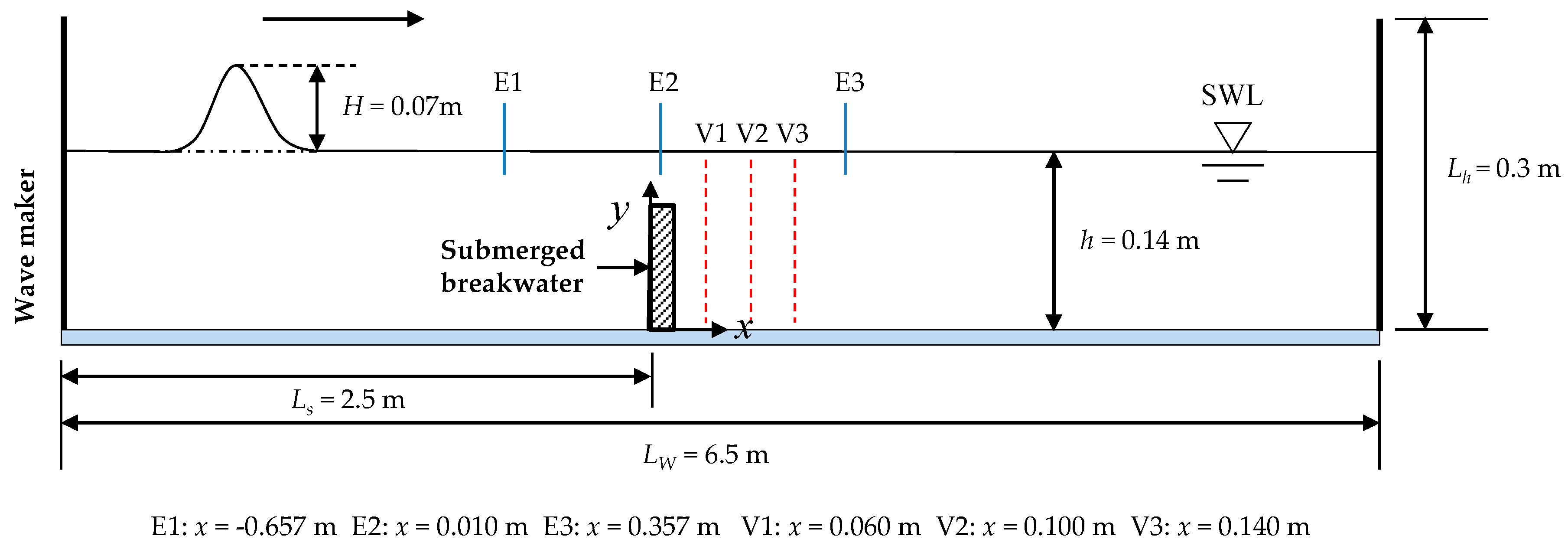
The CPM model is used to study the experimental case of solitary wave interaction with a submerged bottom-mounted breakwater in Wu et al. [15]. Figure 1 is the schematic view of this example, in which the length of the wave flume is 6.5 m, the water depth h = 0.14 m and the rectangular structure (dimension 0.1 m × 0.02 m) located 2.5 m from the home position of the wave maker. Wu’s experimental study was conducted in the wave flume at Tainan Hydraulics Laboratory, National Cheng Kung University. Wave heights at E1 (x = −0.657 m), E2 (x = 0.010 m) and E3 (x = 0.357 m) were measured by wave gauges. The wave profile and velocity filed in a certain area at the leeward of the breakwater were measured by a PIV system. The solitary wave was produced by a translational wave maker, whose motion was generated by the procedure presented in Goring [37]. In CPM simulations, stationary particles of initial particle distance L0 = 0.0025 m are generated in the whole domain. Using the approach introduced in Section 2.3 to move the wave maker in the described way, a solitary wave can be produced. A fixed time step ∆t = 0.0005 s is adopted to satisfy the Courant condition. The CPM results of wave elevations at E1, E2 and E3, wave profiles and wave velocities at three sections (V1-x = 0.06 m, V2-x = 0.10 m and V3-x = 0.14 m, as shown in Figure 1) are compared with the experimental results of Wu et al. [15].
4. Results and Discussions
4.1. Wave Transmission and Reflection
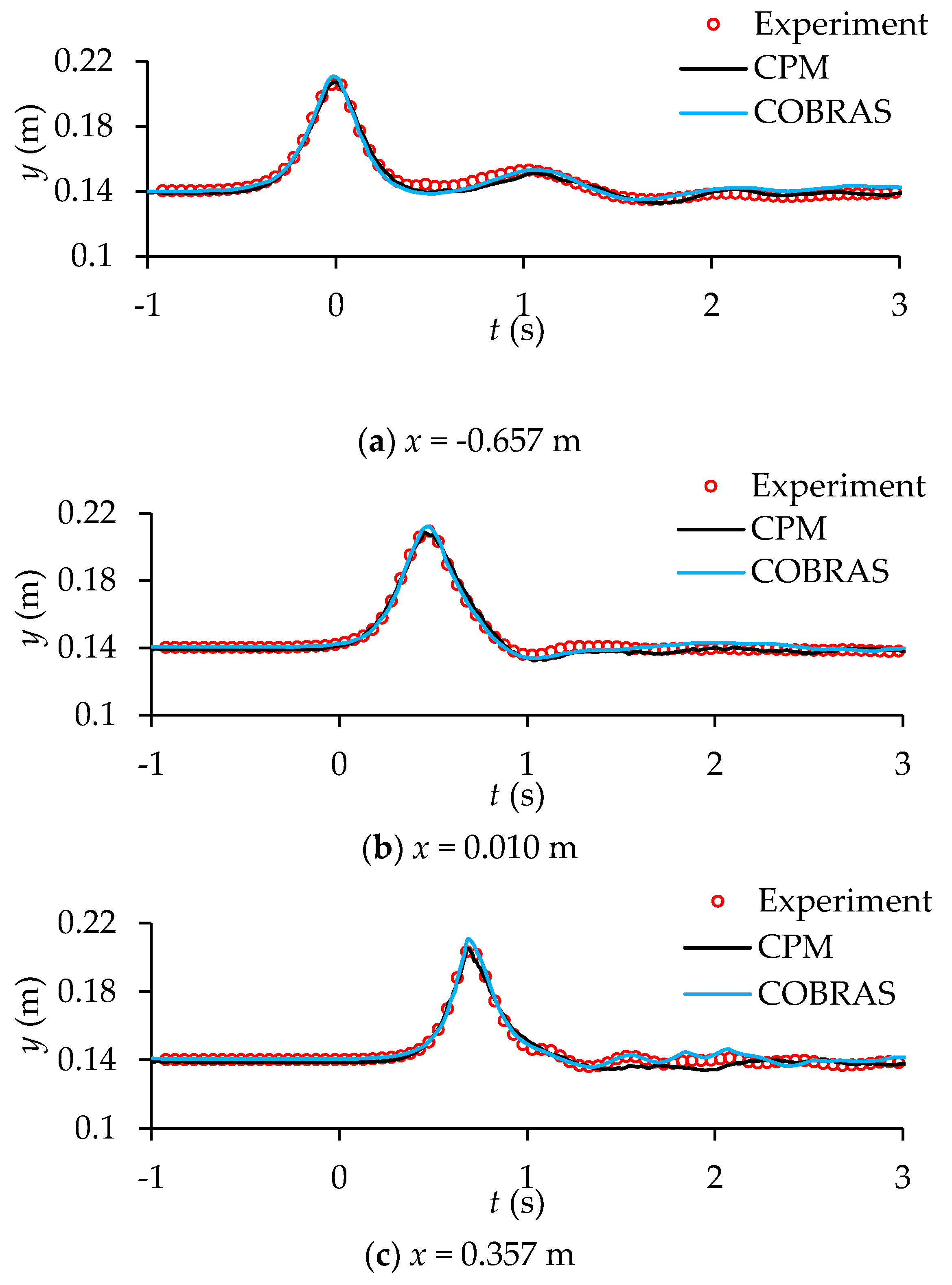
The wavemaker generates a solitary wave of wave height of H = 0.07 m, which propagates forward. The wave elevations just in front of (E1), at the location of (E2) and just behind of (E3) the breakwater is presented in Figure 2. The time when the solitary wave crest occurs at E1 is t = 0 s. In general, the CPM results and the COBRAS numerical results of Wu et al. [15] match quite well and are in a good agreement with Wu’s experimental data [15]. The relative differences of these two sets of numerical wave crests against the experimental data are presented in Table 1. The maximum difference is 3.1% for COBRAS and 0.4% for CPM. Both numerical models are very accurate in predicting the wave elevations. From the next section on, the capability of CPM in reproducing the wave breaking process and tracking the particle trajectories will be demonstrated.
The solitary wave-breakwater interaction happens when the wave approaches the structure. The wave crests at E1 and E3 are treated as the amplitudes of the incident and transmitted waves. Since most of the energy of a solitary wave concentrates on the bulge part of the wave, the ratio of the transmitted and incident wave heights, i.e., Ht/Hi, is used as an indicator of the wave transmission. Based on this, the wave transmission coefficient of this case is 92.6%. The breakwater also reflects part of the wave, which is manifested in the second crest of wave elevation at E1 that occurs at around t = 1 s. With the same argument for the wave transmission, the wave reflection coefficient is evaluated by the ratio of the reflected and incident wave heights, i.e., Hr/Hi. It is computed to be 17.7% for this case. Analytical solutions have been derived for estimating the wave transmission (Equation 4.8 in [38]) and reflection (Equation (11) in [13]) coefficients of a solitary wave propagating rectangular submerged obstacles. Based on these equations, the wave transmission and reflection coefficients of this case are 95.3% and 18.1%, the relative differences between which and the CPM solutions are 2.8% and 2.2%, respectively.
4.2. Fluid Characteristics of Wave-Structure Interaction
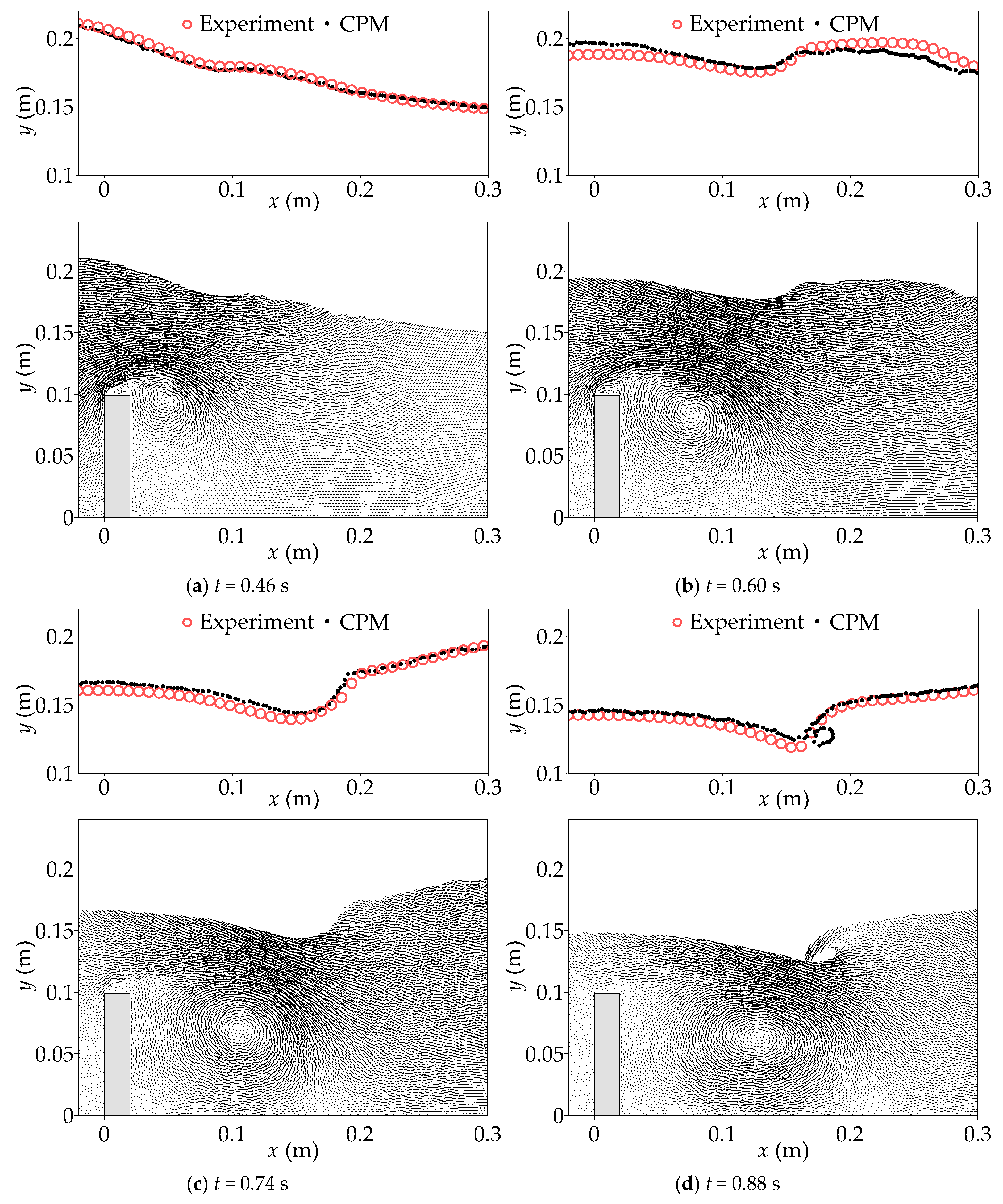
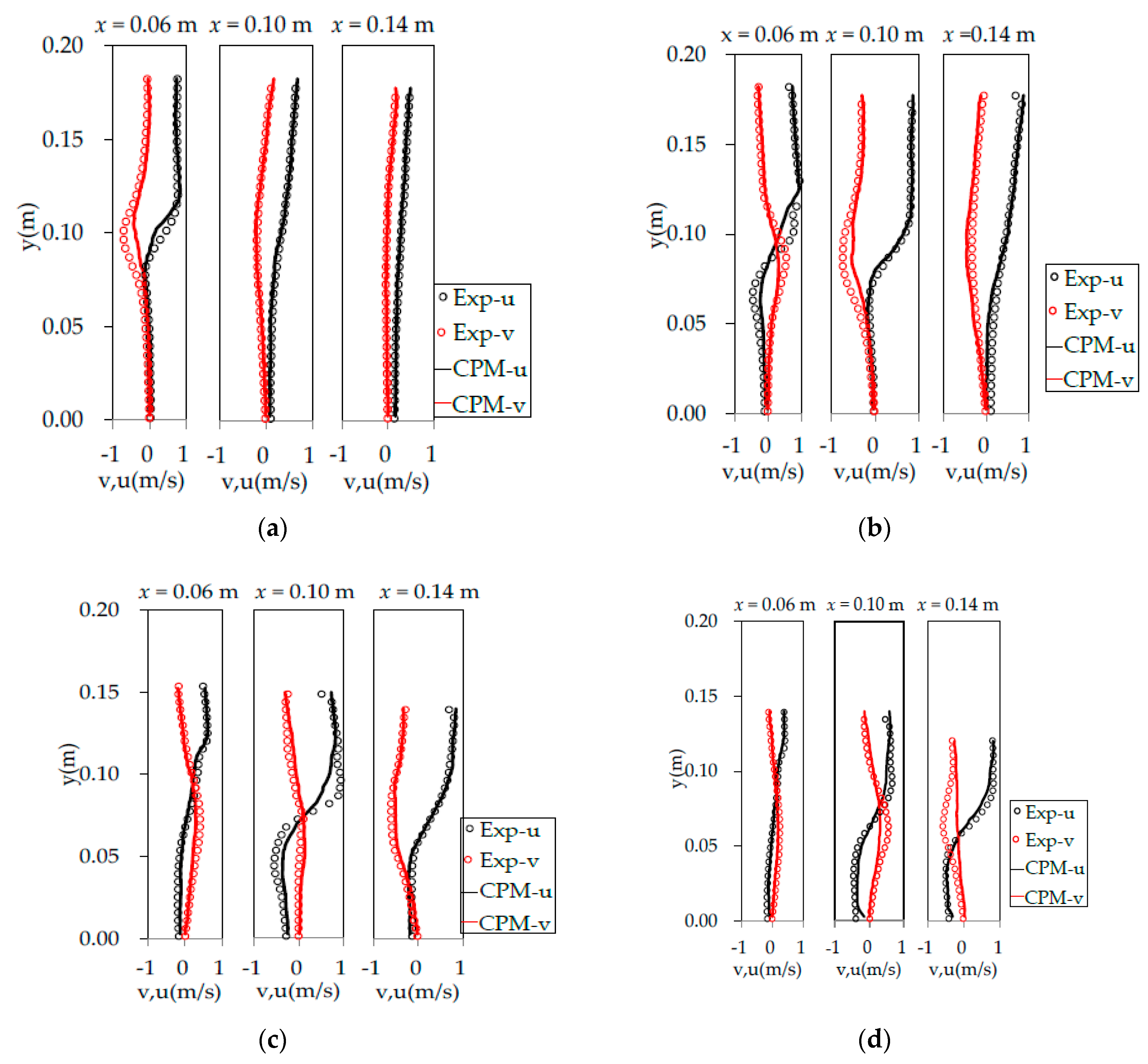
When the wave approaches the breakwater, the wave accelerates due to the blockage of part of the flume section. This leads to a jet flow toward the leeward side of the breakwater. Accompanied is a clockwise vortex behind and at an elevation near the crest of the breakwater. These phenomena can be clearly seen from the velocity profile at t = 0.46 s as shown in Figure 3a. The jet flow impinges the main water body behind the breakwater. Due to the velocity of the main water body being smaller than that of the impinging flow, the elevation of the water body is raised (see Figure 3b). The raised water body and the crest of the incoming jet flow form the double crests. This is the so-called crest-crest exchange phenomenon [15,39]. As the main crest of the solitary wave propagates downstream, the jet flow impingement increases the steepness of the tail of the transmitted wave (see the wave profile at t = 0.74 s). The impinging flow continuously reduces the water elevation of the impinging location and causes the tail surface to break in the direction opposite to that of the main wave direction (Figure 3d). In this process, the vortex develops in size and moves downstream with the wave. Specifically, the vortex occupies the area of 0.2 m × 0.1 m behind the breakwater at t = 0.88 s. It is noteworthy that the CPM model has accurately reproduced the experimental wave profiles at the time instants discussed above. And the predicted velocity distributions at sections V1, V2 and V3 are in a reasonably good agreement with the experimental results as shown in Figure 4. Although some discrepancies exist near the center of the vortex region, the numerical model is able to capture the key phenomena during this process. This shows the satisfactory accuracy of CPM.
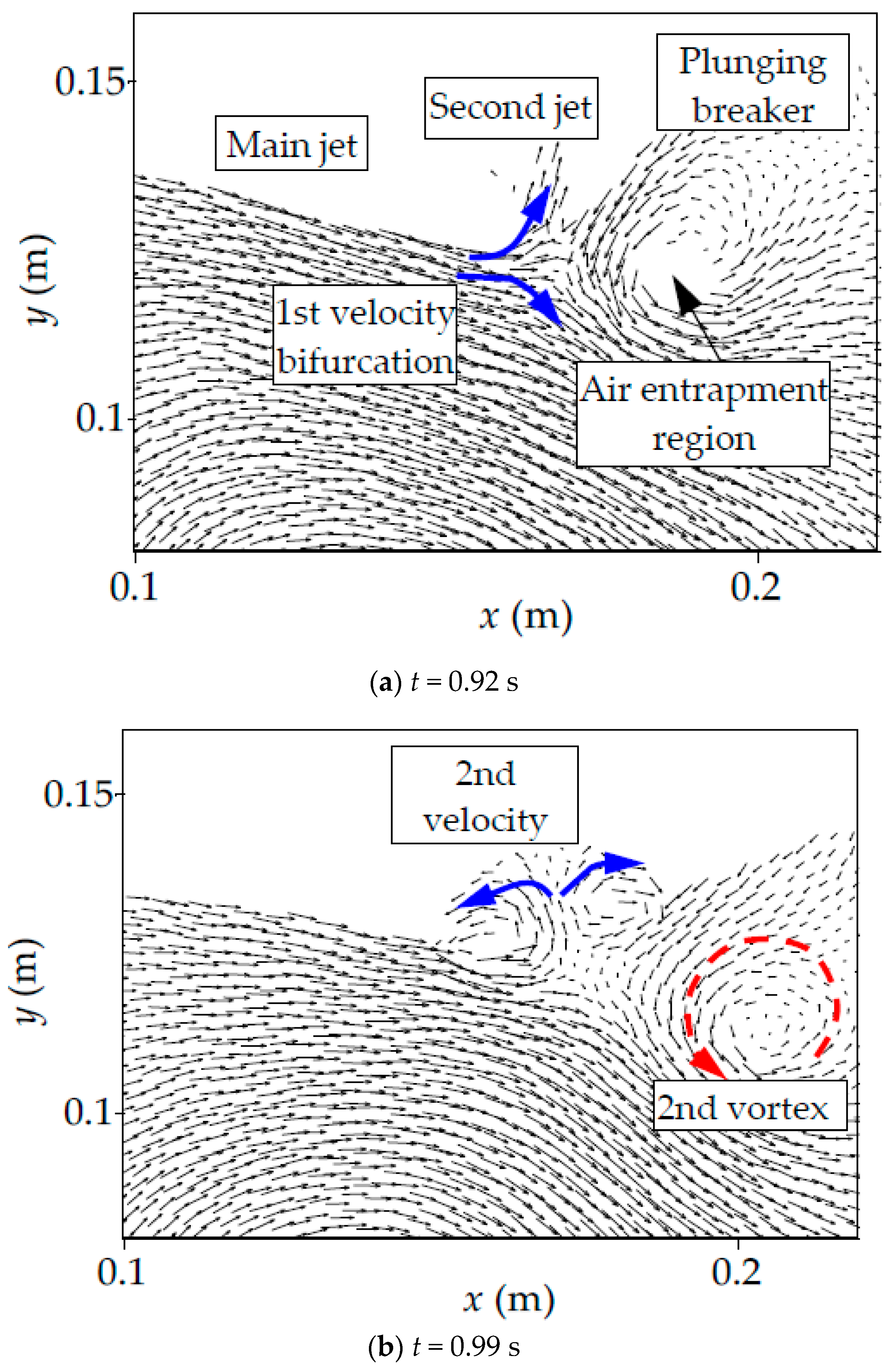
The backward (in terms of the main wave direction) plunging breaker interacts with the forward main jet flow, inducing energetic and complicated local fluid motion. Specifically, the impingement of the plunging breaker on the main jet causes a velocity bifurcation, as shown by the bent arrows in Figure 5a. The fluid with an upward velocity component forms a second jet, while the majority of the main jet maintains the original moving direction and merges into the main water body. The second jet rises to an elevation higher than the crest of the plunging wave because the wave kinetic energy is converted to the potential energy, and then splits into two parts (see Figure 5b). The leftward part overturns and impinges on the main jet flow again, and the rightward part impinges on the plunging breaker. All violent wave-breaking scenarios during this process dissipate wave energy. Another interesting phenomenon accompanying this process is the air entrapment as shown in Figure 5a. Since the present CPM model does not include the air phase, the effects of the air entrapment on the local fluid characteristics are not simulated. To capture this in detail, a two-phase simulation that allows for the compressible air necessitates and is left for the future work. The air entrapment region is occupied by water very quickly because of gravity. The fluid that surrounds this region forms an anti-clockwise vortex as shown in Figure 5b.
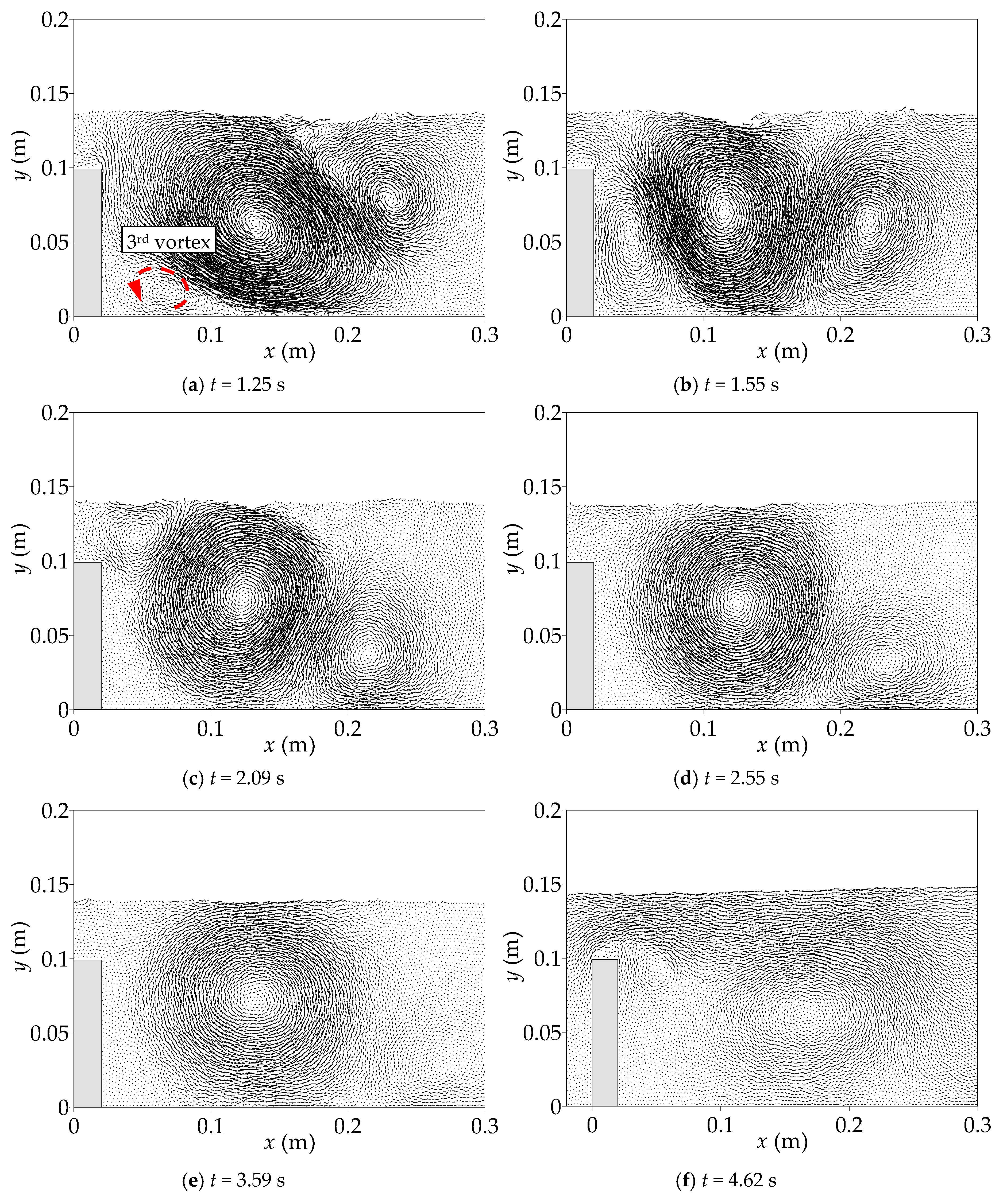
The main vortex induced by the main jet flow and the second vortex initiated by the plunging breaker keep on developing after the main body of the solitary wave passes by this region. While the second vortex is rotating itself, it rotates around the main vortex, liking the movement relationship between a satellite and a planet. When the water at the leeward starts to flow back to the seaward at around t = 1.2 s (manifested in the wave elevation at E2 in Figure 2), a third vortex is initiated near the leeward toe of the breakwater (see Figure 6a). By rotating around the main vortex, this vortex subsequently goes up to the free surface (Figure 6b,c). Due to the energy dissipation induced by fluid viscosity, the third and second vortex disappear at t = 2.55 s (Figure 6d) and t = 3.59 s (Figure 6e), respectively. The backflow goes to the wave paddle and is reflected again. This new incident wave that has a much smaller amplitude pushes the remaining main vortex onshore and generates a small vortex near the crest of the breakwater at the leeward (Figure 6f). These vortexes will disappear eventually under the action of fluid viscous force.
4.3. Trajectories of the Fluid Particles
The vortex transports sediment particles and can cause the failure of structure foundations or excessive sediment deposition, both of which will affect the proper functioning of a submerged breakwater. Since the sediment motion is closely related to fluid motion, this section discusses the trajectories of fluid particles at typical locations, to provide some insights into the possible sediment transportations. Note that, because of the Lagrangian description, the particle method offers convenience for this analysis.
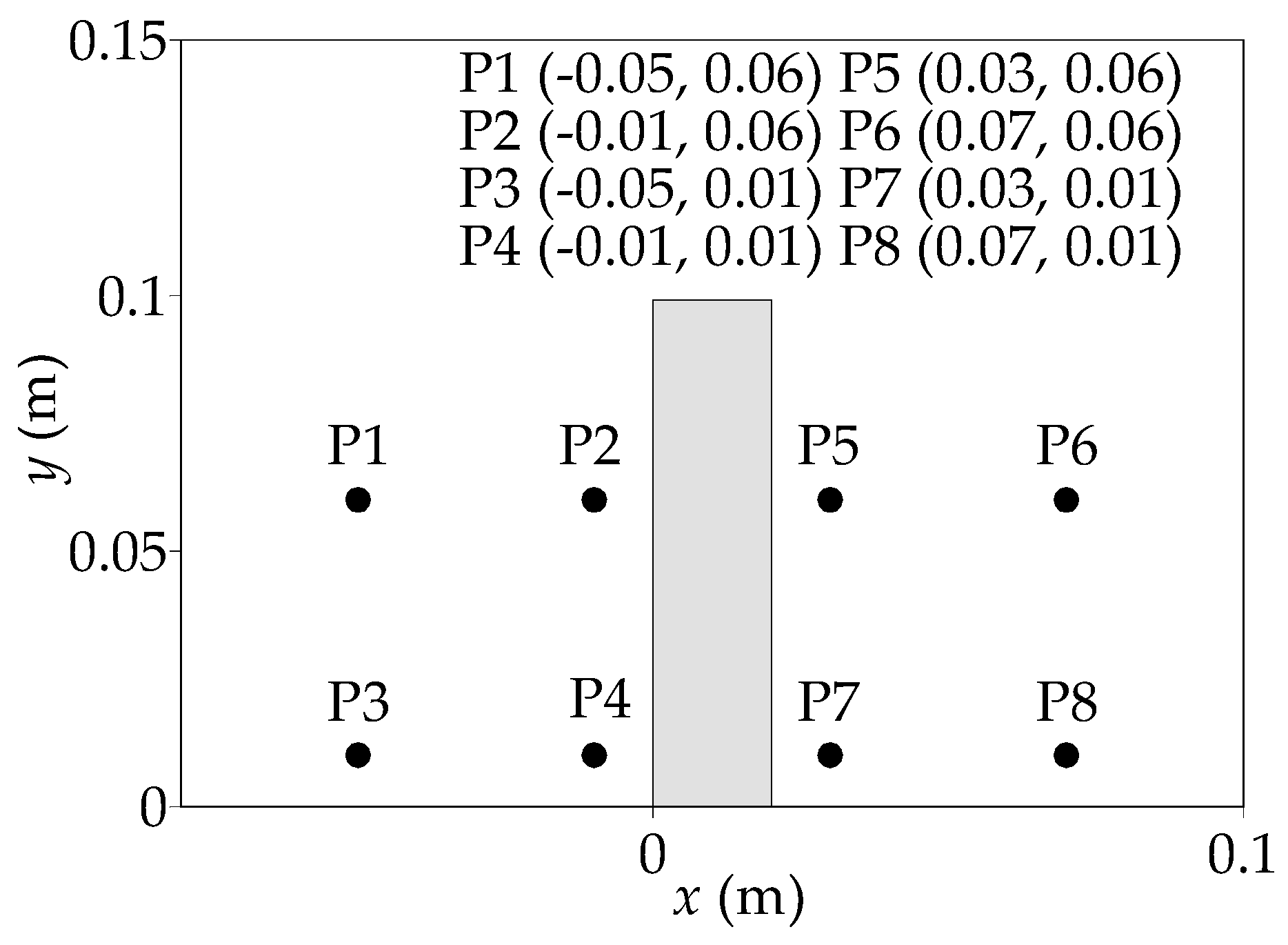
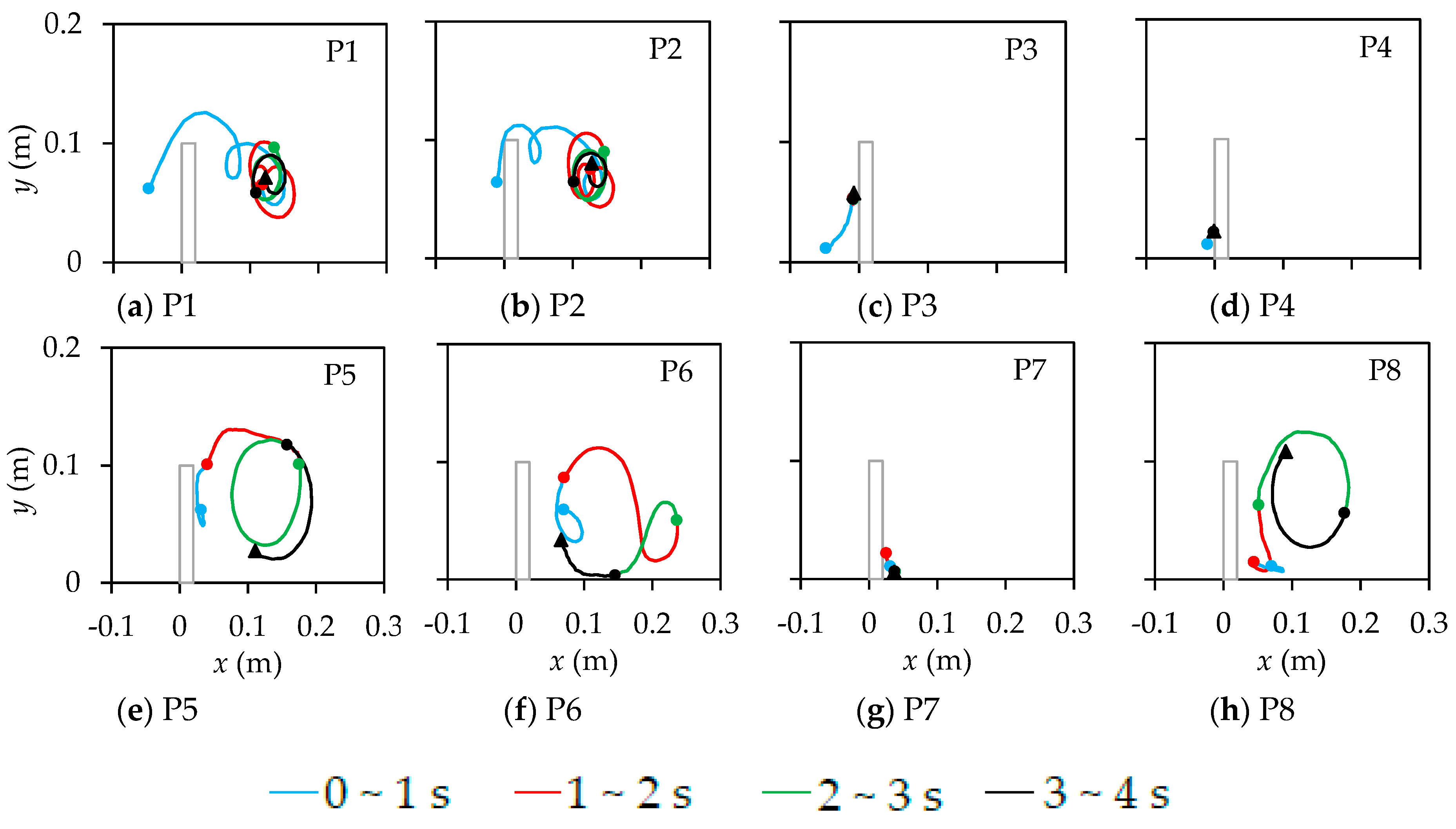
Eight particles (the initial positions shown in Figure 7) at the seaward and leeward sides of the breakwater are traced and the trajectories are shown in Figure 8. Particles 1 and 2, which are initially located at the seaward and at an elevation of half of the breakwater height, go along the onshore direction with the main jet flow because of the vortex and their trajectories display spirals, as shown in Figure 8a,b. Particle 3 moves from a position near the flume bed to an elevation more than half of the breakwater (Figure 8c). The seaward bottom corner of the structure is a stagnation point. Hence, particle 4 that is near to structure toe has a small velocity during this period. However, this particle does move up a distance (Figure 8d). It can be anticipated that, with the actions of some more waves, particles 3 and 4 will go up further and eventually move to the leeward of the breakwater. The trajectories of particles 1 to 4 imply that the running-up component of the wave upon the interaction with the breakwater has the power to move the sediment particles near the seaward toe to the leeward. This will induce the erosion of the breakwater foundation.
The particles originally located at the leeward and at an elevation of half of the breakwater height (i.e., particles 5 and 6) move with the main vortex, and the trajectories are spirals (Figure 8e,f). Particle 8 that initially locates near the flume bed is easily “transported” by the main vortex (Figure 8h). Similar to particle 4, particle 7 (near to the leeward toe of the breakwater) does not have a long trajectory as shown in Figure 8g. The main feature of the water particle trajectories at the lee side of the breakwater is that the vortex flow initiates the sediment particles. With the combined actions of vortexes and incident waves, the sediment particles will be transported onshore and the foundation of the breakwater will be eroded. Therefore, these factors should be considered carefully in practical designs.
5. Influence of Breakwater Dimension on Fluid Characteristics
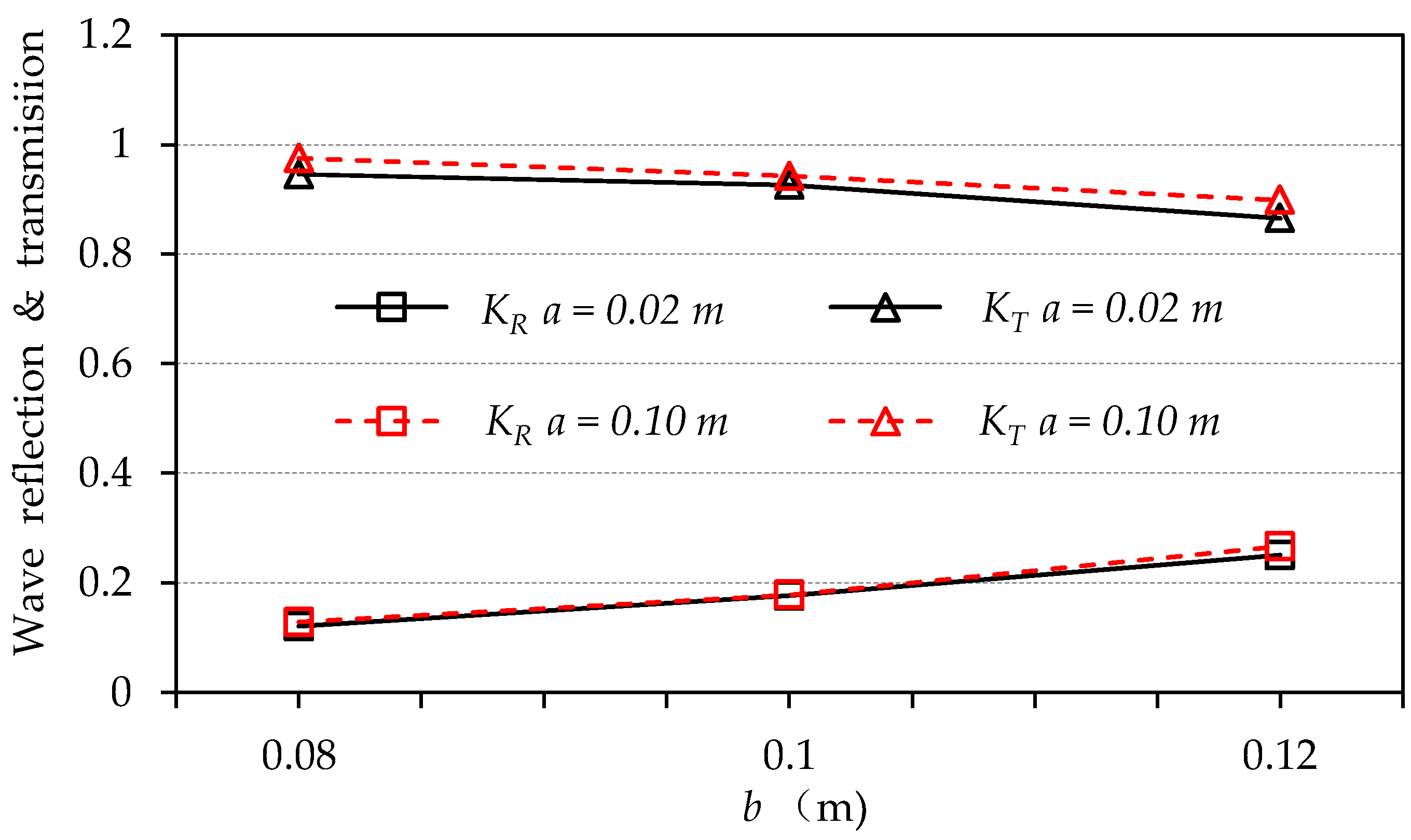
In practical applications, the dimension of a breakwater and the wave conditions are important factors that affect the effectiveness of the breakwater in preventing incident waves and dissipating wave energy. To provide some insights, this section conducts a parametric study by analyzing the wave characteristics of the abovementioned solitary wave interacting with six rectangular submerged breakwaters, whose dimensions are shown in Table 2. The wave transmission (KT) and reflection coefficients (KR) with breakwaters of different dimensions are shown in Figure 9. As can be seen, increasing the breakwater height increases the wave reflection and reduces the wave transmission, while the breakwater width has little effect on wave reflection and transmission.
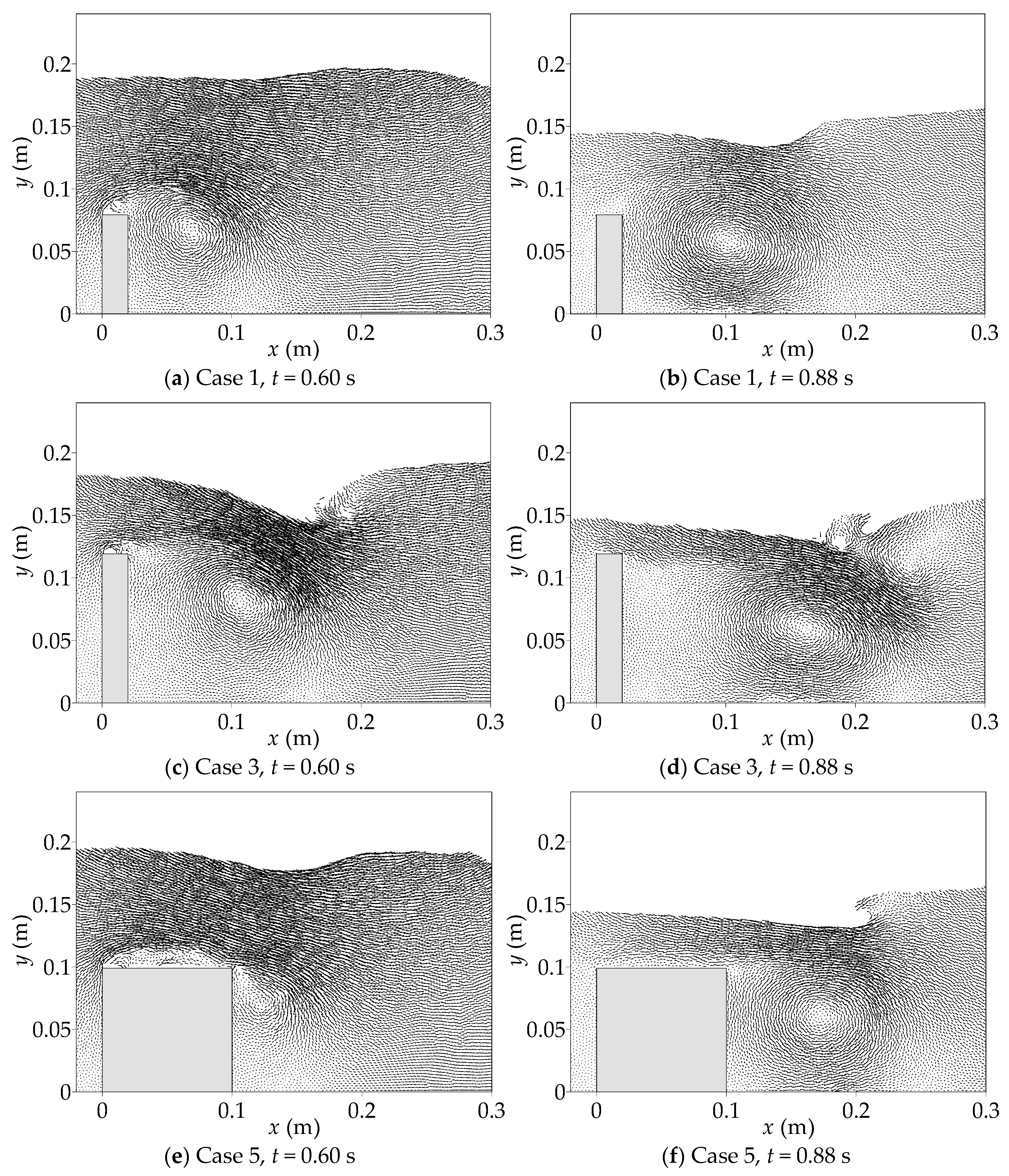
When the breakwater width is fixed, a higher breakwater causes more wave reflections and hence less transmitted waves. However, because of the reduction of the section that the wave goes through, the jet flow that impinges towards the lee side has a larger velocity. This induces breaking waves and vortexes of higher intensity. Besides, the main vortex is further away from the structure because the jet flow ejects further from the crest of the breakwater. These phenomena are manifested by the velocity fields of cases 1 (Figure 10a,b), 2 (Figure 3b,d) and 3 (Figure 10c,d) at t = 0.60 s and 0.88 s. The strong vortex induces more sediment transportations and hence erosions. In practical designs, therefore, one needs to consider the balance between reflecting more waves and the severity of the erosion at the lee side of the breakwater. The effect of the breakwater width on the flow field is demonstrated by comparing cases 2 and 5 (Figure 10e,f). The key difference is that the main vortex in the case with a wider breakwater is closer to the lee side toe of the breakwater. The practical implementation is that more sediment particles near the structure toe will be initiated and transported away, causing the attached scour as termed in Young and Testik [40]. For a narrow breakwater, since the main vortexes are relatively far from the toe of the breakwater, the sediment particles underneath of the main vortexes are initiated. Some sediments are transported closer to the breakwater and deposited at the lee side toe. This causes the detached scour [40].
6. Conclusions
In this work, the CPM is used to study the solitary wave interaction with rectangular submerged breakwaters. The distinct feature of CPM is that it computes the gradient and Laplacian operators in the governing equations in a way consistent with the Taylor series expansion. This addresses the issue of numerical consistency that exists in some other particle methods and hence enhances the numerical accuracy. The CPM model is used to study a documented experimental case. The wave elevation, wave profile and velocity distributions are in good agreement with the experimental data.
Using the validated numerical model, the process of solitary wave-breakwater interaction is studied in detail. The incident solitary wave turns into a jet flow when passing through the breakwater. The jet flow moves onshore and impinges on the water body at the lee side of the breakwater. Subsequently, a backward plunging wave is generated, the interaction between which and the jet flow induces a second jet. The second jet goes up and then splits into two parts. One part re-impinges on the main jet flow and the other part impinges on the plunging breaker, both of which induce splashes. The wave splitting and merging during the wave breaking process cause the dissipation of wave energy.
The main jet flow induces a big vortex behind the breakwater and the plunging breaker induces a secondary vortex. While both vortexes cause the spin of fluid particles, the second vortex, as a whole, rotates around the main vortex. The vortexes play key roles in transporting sediment particles and dissipating wave energy. The potential or capability of the wave flows around the breakwater to transport sediment particles are further studied by analyzing the trajectories of fluid particles. In general, the waves tend to move the seaward sediment particles near the breakwater to the leeward, and transport the sediment leeward particles further onshore.
The influence of the breakwater dimension on the fluid flow around the breakwater is studied. It is found that a higher breakwater causes more wave reflection and hence fewer waves go through the structure. Although the breakwater width has a negligible effect on wave reflection and transmission, the vortex distribution and the associated toe scour pattern are closely related to the width of a breakwater. Specifically, the detached scour is more likely to happen for a narrow breakwater and the attached scour for a wide breakwater.
Author Contributions
Conceptualization, Y.R., M.L. and P.L.; methodology, Y.R., M.L. and P.L.; simulation and data analysis, Y.R. and M.L.; writing—original draft preparation, Y.R. and M.L.; writing—review and editing, Y.R. and M.L.
Funding
This research work is supported by the Open Funding SKHL1710 and SKHL1712 from the State Key Laboratory of Hydraulics and Mountain River Engineering in Sichuan University, China.
Acknowledgments
The authors thank Yun-ta Wu at Tamkang University and Shih-Chun Hsiao in National Cheng Kung University for providing the experimental data as presented in Section 4.
Conflicts of Interest
The authors declare no conflict of interest.
References
- Relief Web. Available online: https://reliefweb.int/disaster/eq-2018-000156-idn (accessed on 20 November 2018).
- MSF. Available online: https://www.msf.org.uk/country/indonesia-tsunami-response (accessed on 20 November 2018).
- CoastalWiki. Available online: http://www.coastalwiki.org/wiki/Detached_breakwaters#Reasons_for_selecting_a_submerged.2Flow_breakwater (accessed on 20 November 2018).
- Synolakis, C.E. The runup of solitary waves. J. Fluid Mech. 2006, 185, 523–545. [Google Scholar] [CrossRef]
- Briggs, M.J.; Synolakis, C.E.; Harkins, G.S.; Green, D.R. Laboratory experiments of tsunami runup on a circular island. Pure Appl. Geophys. 1995, 144, 569–593. [Google Scholar] [CrossRef]
- Madsen, P.A.; Fuhrman, D.R.; Schäffer, H.A. On the solitary wave paradigm for tsunamis. J. Geophys. Res. 2008, 113. [Google Scholar] [CrossRef] [Green Version]
- Qu, K.; Ren, X.Y.; Kraatz, S. Numerical investigation of tsunami-like wave hydrodynamic characteristics and its comparison with solitary wave. Appl. Ocean Res. 2017, 63, 36–48. [Google Scholar] [CrossRef]
- Sté Grilli, P.T.; Losada, M.A. Characteristics of solitary wave breaking induced by breakwaters. J. Waterway Port Coast. Ocean Eng. 1994, 120, 74–92. [Google Scholar] [CrossRef]
- Lin, P.Z.; Chang, K.A.; Liu, L.F. Runup and rundown of solitary waves on sloping beaches. J. Waterway Port Coast. Ocean Eng. 1999, 125, 247–255. [Google Scholar] [CrossRef]
- Chang, K.A.; Hsu, T.J.; Liu, L.F. Vortex generation and evolution in water waves propagating over a submerged rectangular obstacle: Part II: Cnoidal waves. Coast. Eng. 2005, 52, 257–283. [Google Scholar] [CrossRef]
- Huang, C.J. On the interaction of a solitary wave and a submerged dike. Coast. Eng. 2001, 43, 265–286. [Google Scholar] [CrossRef]
- Liu, P.L.F.; Albanaa, K. Solitary wave runup and force on a vertical barrier. J. Fluid Mech. 2004, 505, 225–233. [Google Scholar] [CrossRef]
- Lin, P.Z. A numerical study of solitary wave interaction with rectangular obstacles. Coast. Eng. 2004, 51, 35–51. [Google Scholar] [CrossRef]
- Hsiao, S.C.; Lin, T.C. Tsunami-like solitary waves impinging and overtopping an impermeable seawall: Experiment and RANS modeling. Coast. Eng. 2010, 57, 1–18. [Google Scholar] [CrossRef]
- Wu, Y.T.; Hsiao, S.C.; Huang, Z.C. Propagation of solitary waves over a bottom-mounted barrier. Coast. Eng. 2012, 62, 31–47. [Google Scholar] [CrossRef]
- Monaghan, J.J. Simulating free surface flows with SPH. J. Comput. Phys. 1994, 110, 399–406. [Google Scholar] [CrossRef]
- Liu, G.R.; Liu, M.B. Smoothed Particle Hydrodynamics: A Meshfree Particle Method; World Scientific: Singapore city, Singapore, 2003. [Google Scholar]
- Koshizuka, S.; Nobe, A.; Oka, Y. Numerical analysis of breaking waves using the moving particle semi-implicit method. Int. J. Numerical Methods Fluids 1998, 26, 751–769. [Google Scholar] [CrossRef]
- Marrone, S.; Antuono, M.; Colagrossi, A.; Colicchio, G.; le Touzé, D.; Graziani, G. δ-SPH model for simulating violent impact flows. Comput. Methods Appl. Mech. Eng. 2011, 13–16, 1526–1542. [Google Scholar] [CrossRef]
- Lind, S.J.; Xu, R.; Stansby, P.K.; Rogers, B.D. Incompressible smoothed particle hydrodynamics for free-surface flows: A generalised diffusion-based algorithm for stability and validations for impulsive flows and propagating waves. J. Comput. Phys. 2012, 231, 1499–1523. [Google Scholar] [CrossRef]
- Liu, X.; Lin, P.; Shao, S. An ISPH simulation of coupled structure interaction with free surface flows. J. Fluids Struct. 2014, 48, 46–61. [Google Scholar] [CrossRef]
- Ren, B.; He, M.; Li, Y.; Dong, P. Application of smoothed particle hydrodynamics for modeling the wave-moored floating breakwater interaction. Appl. Ocean Res. 2017, 67, 277–290. [Google Scholar] [CrossRef]
- Amicarelli, A.; Albano, R.; Mirauda, D.; Agate, G.; Sole, A.; Guandalini, R. A Smoothed Particle Hydrodynamics model for 3D solid body transport in free surface flows. Comput. Fluids 2015, 116, 205–228. [Google Scholar] [CrossRef]
- Gotoh, H.; Khayyer, A. On the state-of-the-art of particle methods for coastal and ocean engineering. Coast. Eng. J. 2018, 60. [Google Scholar] [CrossRef]
- Monaghan, J.J.; Kos, A. Solitary waves on a cretan beach. J. Waterway Port Coast. Ocean Eng. 1999, 125, 145–155. [Google Scholar] [CrossRef]
- Shao, S.; Lo, E.Y.M. Incompressible SPH method for simulating newtonian and non-newtonian flows with a free surface. Adv. Water Resour. 2003, 26, 787–800. [Google Scholar] [CrossRef]
- Zhang, Y.L.; Tang, Z.Y.; Wan, D.C. Simulation of solitary wave interacting with flat plate by MPS method. Chin. J. Hydrodyn. 2016, 31, 395–401. [Google Scholar]
- Huang, Y.; Zhu, C. Numerical analysis of tsunami-structure interaction using a modified MPS method. Nat. Hazards 2015, 75, 2847–2862. [Google Scholar] [CrossRef]
- Khayyer, A.; Gotoh, H.; Shao, S. Enhanced predictions of wave impact pressure by improved incompressible SPH methods. Appl. Ocean Res. 2009, 31, 111–131. [Google Scholar] [CrossRef] [Green Version]
- Koh, C.G.; Gao, M.; Luo, C. A new particle method for simulation of incompressible free surface flow problems. Int. J. Numerical Methods Eng. 2012, 89, 1582–1604. [Google Scholar] [CrossRef]
- Luo, M.; Koh, C.G.; Gao, M.; Bai, W. A particle method for two-phase flows with large density difference. Int. J. Numerical Methods Eng. 2015, 103, 235–255. [Google Scholar] [CrossRef]
- Koh, C.G.; Luo, M.; Gao, M. Modelling of liquid sloshing with constrained floating baffle. Comput. Struct. 2013, 122, 270–279. [Google Scholar] [CrossRef]
- Luo, M.; Koh, C.G. Shared-Memory parallelization of consistent particle method for violent wave impact problems. Appl. Ocean Res. 2017, 69, 87–99. [Google Scholar] [CrossRef]
- Chorin, A.J. The numerical solution of the Navier-Stokes equations for an incompressible fluid. Bull. Am. Math. Soc. 1967, 73, 928–931. [Google Scholar] [CrossRef]
- Dilts, G.A. Moving least-squares particle hydrodynamics II: Conservation and boundaries. Int. J. Numerical Methods Eng. 2000, 48, 1503–1524. [Google Scholar] [CrossRef]
- Liu, X.; Xu, H.; Shao, S. An improved incompressible SPH model for simulation of wave–structure interaction. Comput. Fluids 2013, 71, 113–123. [Google Scholar] [CrossRef]
- Goring, D.G. Tsunamis—The Propagation of Long Waves onto a Shelf. Ph.D. Thesis, California Institute of Technology, Pasadena, CA, USA, 1978. [Google Scholar]
- Sugimoto, N.; Nakajima, N.; Kakutani, T. Edge-layer theory for shallow-water waves over a step–reflection and transmission of a soliton. J. Phys. Soc. Jpn. 1987, 56, 1717–1730. [Google Scholar] [CrossRef]
- Cooker, M.J.; Peregrine, D.H.; Vidal, C.; Dold, J.W. The interaction between a solitary wave and a submerged semicircular cylinder. J. Fluid Mech. 1990, 215, 1–22. [Google Scholar] [CrossRef]
- Young, D.M.; Testik, F.Y. Onshore scour characteristics around submerged vertical and semicircular breakwaters. Coast. Eng. 2009, 56, 868–875. [Google Scholar] [CrossRef]
Figure 1.
Schematic view of the solitary wave propagating over a submerged breakwater.

Figure 2.
Wave elevations at E1, E2 and E3: (a) x = −0.657 m; (b) x = 0.010 m; (c) x = 0.357 m.

Figure 3.
Wave profiles and velocity fields at typical time instants: (a) t = 0.46 s; (b) t = 0.60 s; (c) t = 0.74 s; (d) t = 0.88 s.
Figure 3.
Wave profiles and velocity fields at typical time instants: (a) t = 0.46 s; (b) t = 0.60 s; (c) t = 0.74 s; (d) t = 0.88 s.

Figure 4.
Horizontal and vertical velocity distributions at the sections of x = 0.06 m, x = 0.10 m and x = 0.14 m at typical time instants: (a) t = 0.46 s; (b) t = 0.60 s; (c) t = 0.74 s; (d) t = 0.88 s.
Figure 4.
Horizontal and vertical velocity distributions at the sections of x = 0.06 m, x = 0.10 m and x = 0.14 m at typical time instants: (a) t = 0.46 s; (b) t = 0.60 s; (c) t = 0.74 s; (d) t = 0.88 s.

Figure 5.
The interaction between the backward plunging breaker and the main jet flow: (a) t = 0.92 s; (b) t = 0.99 s.
Figure 5.
The interaction between the backward plunging breaker and the main jet flow: (a) t = 0.92 s; (b) t = 0.99 s.

Figure 6.
Snapshots of backward plunging breaker and forward jet flow interaction: (a) t = 1.25 s; (b) t = 1.55 s; (c) t = 2.09 s; (d) t = 2.55 s; (e) t = 3.59 s; (f) t = 4.62 s.
Figure 6.
Snapshots of backward plunging breaker and forward jet flow interaction: (a) t = 1.25 s; (b) t = 1.55 s; (c) t = 2.09 s; (d) t = 2.55 s; (e) t = 3.59 s; (f) t = 4.62 s.

Figure 7.
Initial positions of the traced particles.

Figure 8.
Trajectories of eight particles from 0 ~ 4 s: Blue line (0 ~ 1 s), red line (1 ~ 2 s), green line (2 ~ 3 s) and black line (3 ~ 4 s)
Figure 8.
Trajectories of eight particles from 0 ~ 4 s: Blue line (0 ~ 1 s), red line (1 ~ 2 s), green line (2 ~ 3 s) and black line (3 ~ 4 s)

Figure 9.
Wave transmission and reflection coefficients with breakwaters of difference dimensions.

Figure 10.
Velocity fields of cases 1, 3 and 5 at t = 0.60 s and t = 0.88 s: (a) Case 1, t = 0.60 s; (b) Case 1, t = 0.88 s; (c) Case 3, t = 0.60 s; (d) Case 3, t = 0.88 s; (e) Case 5, t = 0.60 s; (f) Case 5, t = 0.88 s.
Figure 10.
Velocity fields of cases 1, 3 and 5 at t = 0.60 s and t = 0.88 s: (a) Case 1, t = 0.60 s; (b) Case 1, t = 0.88 s; (c) Case 3, t = 0.60 s; (d) Case 3, t = 0.88 s; (e) Case 5, t = 0.60 s; (f) Case 5, t = 0.88 s.


Table 1.
Relative differences between the numerical and experimental results of wave crests at E1, E2 and E3.
Table 1.
Relative differences between the numerical and experimental results of wave crests at E1, E2 and E3.
| Numerical models | Relative Errors Against Experimental Data in [15] | ||
|---|---|---|---|
| E1 | E2 | E3 | |
| COBRAS in [15] | 2.0% | 1.4% | 3.1% |
| CPM | 0.2% | 0.4% | 0.2% |
Table 2.
Dimensions of six rectangular breakwaters.
| Dimension | Case 1 | Case 2 | Case 3 | Case 4 | Case 5 | Case 6 |
|---|---|---|---|---|---|---|
| Width a (m) | 0.02 | 0.02 | 0.02 | 0.1 | 0.1 | 0.1 |
| Height b (m) | 0.08 | 0.1 | 0.12 | 0.08 | 0.1 | 0.12 |
© 2019 by the authors. Licensee MDPI, Basel, Switzerland. This article is an open access article distributed under the terms and conditions of the Creative Commons Attribution (CC BY) license (http://creativecommons.org/licenses/by/4.0/).
Share and Cite
MDPI and ACS Style
Ren, Y.; Luo, M.; Lin, P. Consistent Particle Method Simulation of Solitary Wave Interaction with a Submerged Breakwater. Water 2019, 11, 261. https://doi.org/10.3390/w11020261
AMA Style
Ren Y, Luo M, Lin P. Consistent Particle Method Simulation of Solitary Wave Interaction with a Submerged Breakwater. Water. 2019; 11(2):261. https://doi.org/10.3390/w11020261
Chicago/Turabian StyleRen, Yaru, Min Luo, and Pengzhi Lin. 2019. "Consistent Particle Method Simulation of Solitary Wave Interaction with a Submerged Breakwater" Water 11, no. 2: 261. https://doi.org/10.3390/w11020261
Note that from the first issue of 2016, this journal uses article numbers instead of page numbers. See further details here.