Spectral Decomposition and a Waveform Cluster to Characterize Strongly Heterogeneous Paleokarst Reservoirs in the Tarim Basin, China

Abstract

The main components of the Ordovician carbonate reservoirs in the Tahe Oilfield are paleokarst fracture-cavity paleo-channel systems formed by karstification. Detailed characterization of these paleokarst reservoirs is challenging because of heterogeneities in characteristics and strong vertical and lateral non-uniformities. Traditional seismic analysis methods are not able to solve the identification problem of such strongly heterogeneous reservoirs. Recent developments in seismic interpretation have heightened the need to describe the fracture-cavity structure of a paleo-channel with more accuracy. We propose a new prediction model for fracture-cavity carbonate reservoirs based on spectral decomposition and a waveform cluster. By the Matching Pursuit decomposition algorithm, the single-frequency data volumes are obtained. The specific frequency data volume that is the most sensitive to the reservoir is chosen based on seismic synthesis traces of well-logging data and geological interpretability. The waveform cluster is then applied to delineate the complex paleokarst systems, particularly the fracture-caves in the runoff zone. This method was applied to the area around Well T615 in the Tahe oilfield, and a paleokarst fracture-cavity system with strong heterogeneity in the runoff zone was delineated and characterized. The findings of this research provide insights for predicting other similar karst systems, such as karstic groundwater and karst hydrogeological systems.

1. Introduction

The Ordovician carbonate paleo-water system in the Tahe Oilfield was mainly formed during the Hercynian period. Influenced by multi-phase tectonic movement and multiple sea-level rises and falls, the karst superposition reformation was developed. Along the faults, cracks, and weathering crusts, a pale karst reservoir with large caves as the main reservoir space was formed. The karst paleo-channel in the karst water system area is the core of the entire karst reservoir system. The caves, with different scales and forms, are closely related to the ancient river channel.

It is generally thought that the Ordovician fracture-cavity carbonate reservoir was formed by dissolution, with an extremely heterogeneous internal structure and non-uniform lithological properties [1,2,3]. Because of the burial depth of the Ordovician carbonate strata, which exceeds 5500 m [1,2,3,4], the seismic reflection signals of the non-conformable surface are weak and discontinuous, with a relatively low signal-to-noise ratio. Due to the irregular geometry, the associated extreme reservoir heterogeneity, and the low resolution of seismic data, it is difficult to predict the distribution of carbonate reservoirs by single-factor geophysical or geological methods.

Geophysicists have carried out a series of research works on characterizing carbonate reservoirs. Yang used well-driven seismic data reprocessing to improve the seismic images of various karst features, such as caves, cave passages, sinkholes, and eroded valleys and hills at different scales [5]. Zeng et al. used an integrated approach to interpret coalesced and collapsed paleo-cave systems from the unique circular pattern of faults that are associated with seismic bright spots [6]. Dou et al. described a seismic characterization approach integrating core, well-log, and rock physics analyses to reveal a complex subsurface paleokarst system in the San Andres Formation, Permian Basin, West Texas [7]. Li et al. used high-frequency anomalies to identify and describe carbonate fracture-cavity reservoirs, and considered that high-frequency anomalies are a more reliable indicator of hydrocarbon bearing [8]. Taherdangkoo and Abdideh applied a discrete wavelet transform (DWT) to decompose water saturation log data to detect fractured zones and calculate the number of fractures. A relationship was obtained between the signal energy of the water saturation log and the number of fractures [9]. Li et al. combined spectral decomposition with coherence methods to process three-dimensional seismic data in the Tarim Basin to characterize channel characteristics in order to quantify geographical discontinuities at different scales [10]. Li et al. proposed the residual signal Matching Pursuit algorithm by improving the traditional Matching Pursuit algorithm with effective reservoir thickness as a constraint to identify the top boundary of a small-scale carbonate reservoir [11]. Parchkoohi introduced an image-processing workflow to enhance selective edges in seismic attribute volumes stemming from karst sinkholes and locate them in high-quality three-dimensional (3D) seismic images by using circular Hough transforms [12]. Liu et al. proposed a sequential characterization procedure including fault and fracture detection, seismic facies classification, seismic impedance inversion, and lithofacies classification [13]. Lu analyzed a series of outcrops, seismic data, and structures to characterize the spatial geometry of these major faults and their surrounding fractures in detail [14]. Taherdangkoo and Abdideh used a regression analysis to estimate the fracture density in the fractured zone from well-log data [15]. Liu integrated observations from outcrop analogs and concepts from modern karst theory for the mapping and modeling of fractured-cavity reservoirs [16].

However, these methods have their limitations. Some studies ignored the resolution and quality of seismic data when describing fractured-cavity reservoirs in the post-stack profile. Some others did not consider the fact that the responses of different sizes of the fracture-cavity system to frequency components is not the same [5,6,7,11,12,13,16]. Conventional broadband data are good at revealing large-scale stratigraphic information on structural patterns, especially medium-to-large scale features, such as faults, and strata with strong reflection. However, broadband data do not always provide the best insight into a seismic attribute analysis. The seismic response of a given geologic feature is expressed differently at different spectral bands. Often, a particular frequency component carries the information regarding structure and stratigraphy [10,11]. The low-frequency component mainly describes the information on large caves; the high-frequency component highlights the information on small caves controlled by large caves. Even though some studies have considered and used frequency information [10], due to the lack of the constraints on well logs and special depositional environments, the selected sensitive frequency is unreliable. In other studies on the further analysis of sensitive data [8], the portrayal of the reservoir distribution is intermittent and discontinuous. Therefore, at the current stage, there is a lack of accurate and effective methods for the study of fracture-cavity reservoirs.

With the further development of oil and gas, the well-constructed and large-scale karst reservoirs have been drilled, and the relatively small-scale fracture-cavity reservoirs have become the new target for increasing production. In order to quantify small-scale fractured-cavity reservoirs, the frequency unrelated to the target scale should be eliminated to reveal subtle features that may be otherwise buried in the broadband seismic response.

This paper proposes a new model for predicting fracture-cavity carbonate reservoirs based on spectral decomposition and a waveform cluster. Firstly, the spectral decomposition algorithm based on Matching Pursuit is used to extract the different single-frequency data volumes. Then, the single-frequency data volume that is sensitive to the reservoirs is determined by the seismic synthesis records obtained by the well logs and the resolution and continuity of the target layer. Finally, the waveform cluster algorithm is applied to characterize the distribution of the fracture-cavity paleo-channels system on the sensitive single-frequency data. This method was applied to the area around Well T615, and the paleokarst fracture-cavity reservoirs with strong heterogeneity around the karst paleo-channels were delineated and characterized.

2. Geological Background

One-fourth of the karst area on Earth is distributed in China, and one-half of the karst bare area is in northern China [16,19]. The Tahe Oilfield is the largest Paleozoic marine oilfield in China [1,2,3,14,16,20,21,22], covering an area of 2400 square kilometers. The Tahe Oilfield is located on the southwestern slope of the South-Central Akekule Arch (shown in Figure 1b) in the North Uplift (Shaya Uplift) of the Tarim Basin (shown in Figure 1a) [17]. Hydrocarbon reservoirs have been identified in Triassic, Carboniferous, Devonian, and Ordovician strata. The Ordovician paleokarst reservoirs account for approximately 73% of total oil and gas production [23]. From the bottom to the top, the Ordovician strata are divided into the Penglaiba Formation, the Yingshan Formation and the Yijianfang group, the Querbake Formation, the Lianglitage Formation, and the Santamu Formation (shown in Figure 1c) [24].

Large, deep faults and associated folds in the Akekule Arch, forming a large karst slope, have experienced a series of erosion events from Caledonia to the Hercynian period [25]. Due to its long duration, widespread distribution, and great intensity, the early Hercynian karstification event was the most significant karstification phase in the formation of the paleokarst systems in the Tahe oilfield [3]. Groundwater dynamics in karst slopes have vertical infiltration and horizontal movement, and a fracture-cavity system has thus developed. The remaining Ordovician formations are uneven, and the contact relationship is complex. The strata in the northern Tahe Oilfield were denuded, and the Carboniferous Bachu Formation unconformably overlies the Yingshan Formation [14]. These events produced the morphological diversity of the karst cave system, resulting in a large-scale karst geomorphology and underground ancient caves, all of which represent the type of karst landforms observed in Guilin today [2,6].

It is this geological environment that provides a broad reservoir space for the accumulation of oil and gas, guaranteeing the high and stable production of the Tahe Oilfield [26]. Hydrocarbons were first generated in the Manjiaer depression before migrating through a series of deep-seated faults and accumulating within large karstic fault systems, which form the current deep-fracture-cavity reservoirs in the north region of the Tarim Basin [14]. The ancient karst reservoir developed near the unconformity in the Middle and Lower Ordovician strata, with a burial depth that exceeds 5500 m [2,3]. The rock matrix has no reservoir permeability, and the accumulation of oil and gas mainly depends on the development degree of the fracture-cavity system in the strata. Previous studies have shown that paleokarst reservoirs are usually located less than 150 m below the unconformity [27,28]. Being the core of the entire karst system, the karst paleo-channels of multiple scales and different orientations are intertwined with various sizes of fracture-cavity reservoirs [14,26,29]. The fracture-cavity reservoirs are distributed in a random and scattered manner with great complexity [30,31], having an extremely heterogeneous internal structure and non-uniform lithological properties [32,33,34,35].

3. Materials and Methods

3.1. Spectral Decomposition

Morlet is the pioneer in applying spectral decomposition (time-frequency) for seismic interpretation [36]. Partyka used a Short Time Fourier Transform to analyze seismic data to describe the distribution of a reservoir [37]. From then on, spectral decomposition has been widely used in the processing and interpretation of seismic data. Spectral decomposition can be used to evaluate changes in bed thickness and lateral heterogeneity with higher resolution than the traditional quarter-wavelength theory [38]. Decomposing a seismic trace into time-variant frequency spectra allows us to draw inferences about seismic events in terms of layer thickness, rock properties, and stratification [39].

Spectral decomposition can generate time-dependent amplitude data as a function of instantaneous frequencies and phases [37,40,41]. In 1946, the British physicist Dennis Gabor proposed the Gabor transform, laying the foundation for time-frequency analysis. The Gabor transform is a special form of the short-time Fourier transform (STFT) when it has a Gaussian window. In 1974, J. Morlet proposed the Wavelet transform, leading the application of time-frequency analysis. The Wavelet transform is a time-frequency localization method with a variable window shape and variable time and frequency windows. It is suitable for detecting abrupt signals in a normal signal [9].

The advantage of time-frequency analysis over the traditional Fourier transform is that time-frequency analysis can obtain the trend of frequency as it changes with time, which means the instantaneous frequency and phase with their amplitudes at each moment. The Fourier transform is a global transformation that only knows what frequency components are included in a signal instead of the time of occurrence of each frequency. The signals that are greatly different in the time-domain may have exactly the same frequency spectrum when transformed by a Fourier analysis.

The current popular spectral decomposition algorithms can be categorized into two classes: (1) simple projection methods; and (2) computationally intensive least-squares methods [42]. Common projection methods include the short-time Fourier transform (STFT) [37,43], the continuous wavelet transform (CWT) [40,44,45], and the S-transform (ST) [46,47,48]. The least-squares approaches include Matching Pursuit (MP) algorithms [42,49] and other sparsity promoting inversion methods [50]. The least-squares methods are intended to overcome the windowing effect of the projection approaches. Spectral decomposition is a non-unique process, and different spectral decomposition methods produce time-frequency spectra with different time and frequency resolutions.

STFT is the most basic form of spectral decomposition. Although STFT has many successful applications [37,51,52], it has insufficient capacity to analyze signals with different structures and sizes because the time and frequency resolution of STFT is determined by the size of the sliding window [53]. Another disadvantage of a short window is that the side lobes of arrivals appear as distinct events in the time-frequency analysis. If the time window is lengthened to improve the frequency resolution, multiple events in the window will introduce notches that dominate the spectrum. Long windows thus make it very difficult to ascertain the spectral properties of individual events [49].

In the following part of this section, we will discuss and compare the time-frequency results obtained by the Continuous Wavelet Transform, the S Transform, and Matching Pursuit to choose the most suitable method for our project.

3.1.1. Continuous Wavelet Transform

A Wavelet analysis replaces the infinitely long triangular function base of the Fourier transform with a finite-length attenuated wavelet base. When the scaling and shift parameters in a wavelet analysis take continuous changes, it is called a continuous wavelet transform (CWT). Compared to the traditional method of short-time Fourier transform, the CWT method does not require pre-selection of the window length and has no fixed time-frequency resolution in the time-frequency plane [44].

The expression of the CWT is [40]:

$$C\left(a,b;s\left(t\right),\psi \left(t\right)\right)={{\displaystyle \int }}_{-\infty }^{+\infty }s\left(t\right)\frac{1}{\sqrt{a}}{\psi }^{*}\left(\frac{t-b}{a}\right)dt,$$

(1)

where $s$ is the signal; $a$ is a scale factor (corresponding to frequency information); $b$ is a shift factor (corresponding to spatiotemporal information); $\psi$ is wavelet basis; and ‘$\ast$’ is complex conjugate.

Intuitively, by multiplying the signal and the wavelet basis of different scales and shifts, the result of a certain scale at a certain shift time can be considered as to how much frequency component corresponding to the current scale is contained in the signal at this moment. In the CWT, wavelets dilate in such a way that the time support changes for different frequencies. A smaller time support increases the frequency support, which shifts toward higher frequencies. Similarly, a larger time support decreases the frequency support, which shifts toward lower frequencies [44]. Thus, when the time resolution increases, the frequency resolution decreases, and vice versa [54]. The CWT has a high-frequency resolution and low time resolution in the low-frequency part, and a high time resolution and a low-frequency resolution in the high-frequency part.

The workflow of the CWT shown in [38] consists of three steps. First, the seismic trace is decomposed into wavelet components. Then, the complex spectrum of each wavelet is multiplied by the coefficients of its CWT, and the results are added to generate an instantaneous frequency gather. Finally, the set of frequency gathers is classified into a constant frequency cube, a time slice, a horizon slice, and/or a vertical portion. The CWT does not produce a time-frequency spectrum, but instead a time-scale map [55]. A scale represents a frequency band and not a single frequency. The time-scale map does not provide a direct intuitive interpretation of the frequency. To interpret the time-scale map, in terms of a time-frequency map, a number of approaches can be taken [44]. Some researchers have converted a time-scale map into a time-frequency spectrum using the center frequency of the wavelet as the frequency [56,57].

3.1.2. S-Transform

The S-transformation (ST), proposed by the geophysicist Stockwell, is a time-frequency analysis method that combines the characteristics of STFT and CWT. The S-transform has some desirable aspects and good computation speed and is easy to implement [48,58]. ST is an extension of CWT [46], and can be expressed as a “phase correction” of CWT. ST has the ability to adjust the time-frequency resolution according to the frequency level at each time position in an adaptive way. The width of the ST’s window function changes inversely with frequency; that is, the low-frequency time window is wider and has a higher frequency resolution, while the high-frequency time window is narrower and has a higher time resolution.

ST is defined as [58]:

$$\mathrm{S}\left(\tau ,f\right)={{\displaystyle \int }}_{-\infty }^{+\infty }s\left(t\right)\frac{\left|f\right|}{\sqrt{2\pi }}\exp \left[-\frac{{\left(t-\tau \right)}^2{f}^2}{2}\right]\exp \left(-i2\pi ft\right)dt,$$

(2)

where $s$ is the signal, $t$ and $\tau$ are times, $\tau$ is the center point of the window that controls the position of the window on the time axis; and $f$ is the frequency. In the S-transform, the Gaussian window function and the wavelet basis are defined as:

$$g_f\left(t\right)=\frac{\left|f\right|}{\sqrt{2\pi }}\exp \left(-\frac{t^2{f}^2}{2}\right),$$

(3)

$${\omega }_f\left(t\right)=g_f\left(t\right)\exp \left(-i2\pi ft\right).$$

(4)

It can be seen that the wavelet basis in the S-transform is composed of the product of the simple harmonic wave and the Gaussian function. The simple harmonics in the wavelet basis are scaled in the time domain, while the Gaussian function is scaled and shifted. This is different from the continuous wavelet transform, in which the simple harmonics perform the same scaling and shifting as the Gaussian function [46]. The calculation flow of the S-transform is similar to the continuous wavelet transform. The output is also a time-scale map, making it necessary to convert the scale factor to frequency information, such as the dominant frequency [42].

3.1.3. Matching Pursuit

Matching Pursuit Decomposition (MPD) is an adaptive search method based on the principle of maximizing the projection energy. It can decompose any signal into a linear extension of an over-complete wavelet dictionary to obtain sparse components of time series [59]. The over-complete wavelet dictionary is a collection of wavelets covering the full ranges of time, frequency, scale, and phase, which is generated by shifting, scaling, and modulating an original wavelet function [60].

The development of MPD aims to overcome the shortcoming of both the window Fourier transform and the wavelet transform [61]. A window Fourier transform cannot describe signal structures with a varying size, because all wavelets have a constant scale that is proportional to the window size. On the contrary, a wavelet transform decomposes a signal over time-frequency atoms of varying scales. However, because a wavelet family is built by restricting its frequency parameters to be inversely proportional to the scale, the expansion coefficients in a wavelet frame do not provide precise estimates of the frequency content of waveforms whose Fourier transform is well-localized, especially at high frequencies [53]. In MPD, signal structures are represented by wavelets that match their time-frequency signature, with better local adaptation and a better time-frequency resolution [62,63,64,65].

The mathematical representation of MPD is [59]:

$$f\left(t\right)={\displaystyle \sum }_{n=0}^{N-1}{a}_n{g}_{{\gamma }_n}\left(t\right)+R^{N}f,$$

(5)

where $a_n$ is the weight of the nth wavelet $m_{{\gamma }_n}$, $R^{N}f$ is the residual with $R^{\left(0\right)}f=f$, and ${\left(g_{{\gamma }_n}\left(t\right)\right)}_{n\in N}$ is a complex-valued Gabor wavelet defined as [53]:

$$g_{\gamma }\left(t\right)=\omega \left(\frac{t-\mu }{\sigma }\right)\exp \left[\mathrm{i}\left(\mathsf{\omega }\left(\mathrm{t}-u\right)+\varnothing \right)\right],$$

(6)

where $w\left(t\right)$ is a Gaussian window, $u$ is the time delay, $\sigma$ is the spread in the time axis(scale), $\mathsf{\omega }$ is the center frequency, and $\varnothing$ is the phase shift. Thus, a Gabor wavelet is characterized by four parameters $\gamma =\left\{\mu ,\sigma ,\omega ,\varnothing \right\}.$

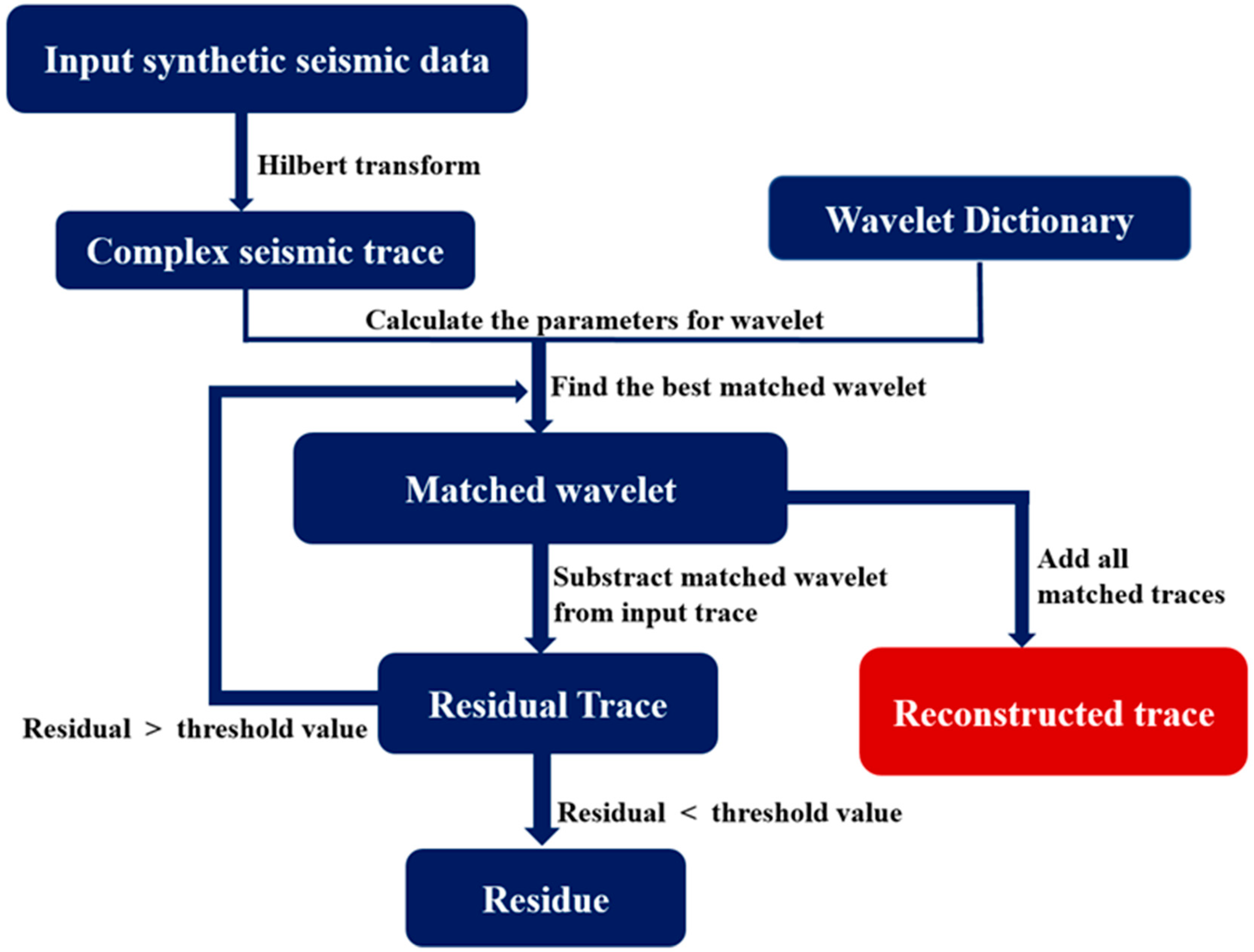
Castagna and S. Sun summarized the flow of MPD as follows [66] (shown in Figure 2). The wavelet dictionary is cross-correlated with the seismic trace, and then the projection of the best-correlated wavelet on the seismic trace is subtracted from the seismic trace. The wavelet dictionary is then cross-correlated with the residual, and the best-correlated wavelet projection is subtracted again. This process is iteratively repeated until the energy of the residual falls below an acceptable threshold. The process will converge as long as the wavelet dictionary satisfies the simple admissibility condition. The output is a list of wavelets with their respective arrival times and amplitudes. With the superposition of wavelet spectra, the wavelet list can be easily converted to a time-frequency analysis.

The process above is computation-intensive. In order to improve the efficiency, we modify the details of the decomposition. In every iteration, we estimate the four parameters ${\gamma }_n=\left\{{\mu }_n,{\sigma }_n,{\omega }_n,{\varnothing }_n\right\}$ efficiently, but approximately.

(1)

Set the time of the maximum envelope of the complex trace to be the time delay ${\mu }_n$, the instantaneous frequency to be the center frequency ${\omega }_n$, and the instantaneous phase to be the phase ${\varnothing }_n$.

(2)

Then, use Equation (7) to search for the optimal parameter ${\sigma }_n$ over a group of preselected, uniformly distributed $\mathsf{\sigma }$ values with fixed ${\mu }_n,{\omega }_n,{\varnothing }_n$ values.

$$g_{{\sigma }_n}\left(t\right)=arg \underset{{\sigma }_n\in \sigma }{\max }\frac{|\langle R^{\left(n\right)}f,g_{{\sigma }_n}\rangle |}{\Vert g_{{\sigma }_n}\Vert }$$

(7)

where $\langle R^{\left(n\right)}f,g_{{\sigma }_n}\rangle$ denotes the inner product of functions $R^{\left(n\right)}f$ and $g_{{\sigma }_n}$, and $\Vert g_{{\sigma }_n}\Vert =\sqrt{\langle g_{{\sigma }_n},g_{{\sigma }_n}\rangle }$.

(3)

Update these four parameters for an optimal wavelet $g_{{\gamma }_n}$ by searching within a range D using Equation (8). The searching range around a parameter $\mathsf{\xi }$ is $\left[\mathsf{\xi }-\Delta \mathsf{\xi }, \mathsf{\xi }+\Delta \mathsf{\xi }\right]$; for instance, $\Delta \mathsf{\mu }$ is the time-sampling interval.

$$g_{{\gamma }_n}\left(t\right)=arg \underset{{\gamma }_n\in D}{\max }\frac{|\langle R^{\left(n\right)}f,g_{{\gamma }_n}\rangle |}{\Vert g_{{\gamma }_n}\Vert }$$

(8)

(4)

After 3, the amplitude of the optimal wavelet $g_{{\gamma }_n}$ is

$$a_n=\frac{|\langle R^{\left(n\right)}f,g_{{\gamma }_n}\rangle |}{\Vert g_{{\gamma }_n}\Vert }.$$

(9)

For comparison, Figure 3 displays the time-frequency spectra generated by CWT, ST, and MP with Morlet Wavelets, defined as [27]:

$$m\left(t\right)=exp\left(-(\frac{ln2}{{\pi }^2}\frac{{\omega }^2{\left(t-\mu \right)}^2}{{\sigma }^2}\right)\exp \left[\mathrm{i}\left(\mathsf{\omega }\left(\mathrm{t}-u\right)+\varnothing \right)\right].$$

(10)

The resolution of both time and frequency, presented in Figure 3a or Figure 3b, is lower than the one in Figure 3c. In our matching pursuit scheme, the scale parameter $\mathsf{\sigma }$ that controls the width of a wavelet is selected adaptively. Therefore, it can even extract narrow wavelets in the signal. For example, a wavelet of 35 Hz around about 260 ms can be clearly identified from the spectrum. In addition, we can also see that the SF can achieve a better frequency resolution than the CWT, especially at a low frequency. This is because the low-frequency time window of ST is wider and has a higher frequency resolution.

Based on the above analysis, we can make a provisional summary. The CWT has the advantage over the STFT because the hidden windows in the wavelet dictionary are frequency-dependent and easy to implement. However, the CWT is a linear time-frequency analysis method and the windowing effect brings about spectral tailing, as shown in Figure 3a. The wavelet function is difficult to select and must be orthogonal. ST combines the advantages of the STFT and the CWT. ST is capable of adaptively adjusting the resolution and its inverse transform is lossless and reversible. However, being also a linear time-frequency analysis method, ST adds spectral tailing and an inaccurate frequency resolution in the high-frequency range, as shown in Figure 3b. MPD does not need to have orthogonal wavelets, but still achieves a superior time and spectral resolution without side-lobe effects, as shown in Figure 3c. Although MP is nonlinear, much like orthogonal expansion, it maintains energy conservation, which guarantees its convergence. The only drawback of common MP is the computational complexity. However, after our detailed modification of the classic MP method, this problem can be solved.

These three methods have been widely used in practical applications of seismic data processing, such as the detection of reservoir shadows [44,53], thin-layer estimation [46], and seismic inversion in attenuating media [67]. More examples for applications of time-frequency decomposition can be found in [10,11,49,68,69,70,71,72,73,74,75]. In particular, Wang developed a multi-channel MP that uses lateral coherence to improve the horizontal consistency [53]. Taherdangkoo and Abdideh applied the discrete wavelet transform to decompose water saturation log data to detect fractured zones and calculate the number of fractures [9].

3.2. Waveform Cluster

The Waveform cluster is a pattern recognition technique often used to analyze seismic waveforms [76,77]. Within a certain interval, the variation in seismic facies gives rise to changes in the amplitude, phase, and frequency of the seismic reflection. The objective of the automatic clustering algorithm is to use such seismic reflections as input and extract the natural clustering of the underlying facies. Within a certain time window, the seismic waveforms belonging to one cluster share the same characteristics and are distinct from those in other clusters [78]. A Waveform cluster can help to visualize the variation in rock properties and the possible relationships between these depositional facies and their seismic response [79,80].

There are many different supervised and unsupervised machine learning algorithms. In supervised training, the labels are predefined and patterns are assigned to them in subsequent training iterations. Examples for applying the supervised method to seismic data can be found in [81,82,83,84,85]. Unsupervised learning is a data-driven method without any a priori information.

The fuzzy C-means cluster (FCM) method is one of the most effective unsupervised clustering algorithms. It learns to discover the natural grouping of patterns without a priori information concerning the membership of a seismic response to a given cluster [86,87]. In most of the classic cluster algorithms, each object is assigned to only one cluster. FCM relaxes this restriction and the object can belong to all of the clusters with a certain degree of membership. This is particularly useful when the boundaries among the clusters are not well-separated and ambiguous. Moreover, the memberships may help us to discover more sophisticated relations between a given object and the disclosed clusters. FCM attempts to find c fuzzy clusters for a set of data points $x_j\in {ℛ}^d, j=1,\dots , N$ while minimizing the cost function [87]:

$$\mathrm{J}\left(\mathrm{U},\mathrm{M}\right)={\displaystyle \sum }_{i=1}^c{\displaystyle \sum }_{j=1}^N{\left({\mu }_{i,j}\right)}^m{D}_{ij}$$

(11)

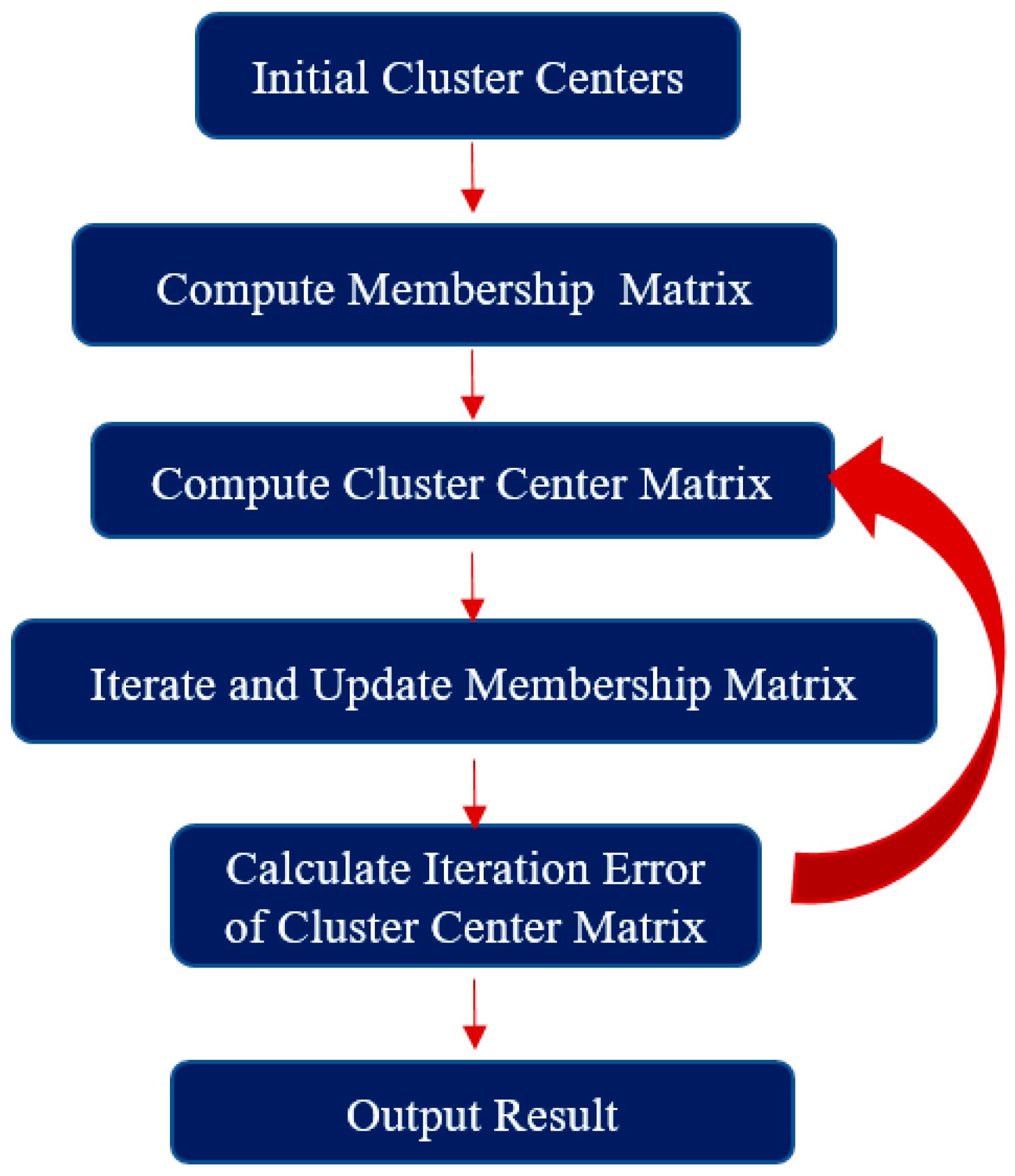
where $\mathrm{U}={\left[{\mu }_{i,j}\right]}_{c\times N}$ is the fuzzy partition matrix and ${\mu }_{i,j}\in \left[0,1\right]$ is the membership coefficient of the jth object in the ith cluster; $\mathrm{M}=\left[m_1,m_2,\dots , m_c\right]$ is the cluster prototype (mean or center) matrix; $\mathrm{m}\in \left[1,\infty \right)$ is the fuzzification parameter and usually is set to 2; and $D_{ij}=D\left(x_j, m_i\right)$ is the distance measure between $x_j$ and $m_i$, for instance, the Euclidean $L_2$ norm distance function. The basic flow of the fuzzy C-means cluster for the waveform is as follows (shown in Figure 4):

(1)

Select the time window to extract the waveforms, $x_j\in {ℛ}^d, j=1,\dots , N$ where $x_j$ is the $j$th waveform in the time window, $d$ is the time sampling number, and $N$ is the number of waveforms;

(2)

Select appropriate values for $m$ and $c$ and a small positive number $\mathsf{\epsilon }$. Initialize the prototype matrix M randomly and set the step variable t = 0.

(3)

Calculate (at t = 0) or update (at t > 0) the membership matrix $\mathrm{U}$ by:

$${\mu }_{ij}{}^{\left(t+1\right)}=1/({\displaystyle \sum }_{l=1}^c{\left(D_{lj}/D_{ij}\right)}^{1/\left(1-m\right)}), for i=1,\dots ,c and j=1,\dots , N.$$

(12)

(4)

Update the prototype matrix M by:

$$m_i{}^{\left(t+1\right)}=({\displaystyle \sum }_{j=1}^N{\left({\mu }_{ij}{}^{\left(t+1\right)}\right)}^m{x}_j)/{\displaystyle \sum }_{j=1}^N{\left({\mu }_{ij}{}^{\left(t+1\right)}\right)}^m), for i=1,\dots ,c.$$

(13)

(5)

Repeat steps 2–3 until $M^{\left(t+1\right)}-M^{\left(t\right)}<\epsilon$. The $j$th waveform is assigned to the $l$th cluster if ${\mu }_{l,j}$ is the maximum of all ${\mu }_{i,j}, i=1,\dots ,c.$

The result is a map of the seismic facies. The clusters of seismic facies provide interpreters with meaningful insights into the structure underlying the seismic data. The natural cluster structure can be related to stratigraphic features or reservoir properties by extracting information about changes in strata, faults, fluid, fractures, lithology, and lithofacies. These stratigraphic features and reservoir properties, when further combined with drilling and logging data, can improve the prediction accuracy in exploration and development in oilfields.

4. Results and Discussions

The study area locates in Block 7 of the Tahe Oilfield, centered on the T615 Well (shown in Figure 1b). The seismic data used is a 3D post-stack dataset with a grid size of 15 × 15 m covering 15.5 square kilometers (4.125 km long and 3.75 km wide). Well-logging data from 10 vertical wells helps to provide sufficient information to characterize fractures and caves in the target strata. Our goal is to use the proposed methods to analyze the spatial distribution of a fracture-cavity paleo-channel reservoir.

4.1. Choose the Reservoir-Sensitive Single-Frequency Data

In the conventional spectral decomposition process, the considered appropriate single-frequency data are generally chosen by experience, and lack geological constraints. The reliability of the suitable single-frequency data has a complex relationship with the surrounding environment of the target reservoir, the strength of the reflection events, and the size of the target reservoir. As for geomorphology, the fracture-cave varies in size, distributes in a random, dispersed, and discontinuous manner, and intertwines with paleo-channels of different scales and different strikes [32,33,34,35]. In addition, the lithological characteristics of the study area are mainly controlled by dissolution with extremely strong heterogeneity. Most importantly, the Ordovician carbonate strata are deeply buried, the seismic response of the non-conformable surface is weak and discontinuous, and the main frequency and signal-to-noise ratio (SNR) are relatively low [1,2,3,4]. Therefore, it is preliminarily speculated that the sensitive frequency we selected should be slightly higher than the main frequency of the seismic data, but not too high because of the limitation of signal quality and strength.

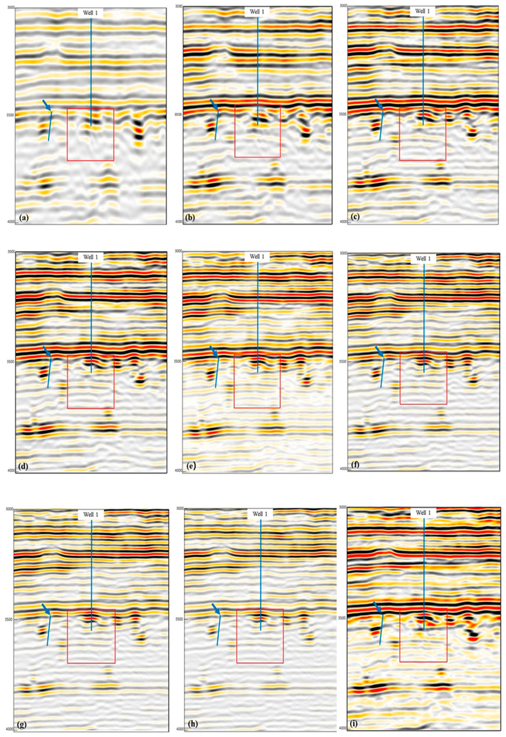
Figure 5i shows a full-band seismic profile in which the target reservoir is between 3.4 and 3.7 s in time with strong heterogeneity. The geomorphological features around the target reservoir show that the reflection of the paleo-channel has a “pull-down” feature, the channel exhibits strong lateral heterogeneity, and the reflection characteristics of the “beads” develop longitudinally. Although controlled by the diving datum and hydrodynamic changes, the paleo-channel’s morphological structure and scale formed along the layers and fracture zones are very different, but the common feature is the layered reflection structure of the cave (shown in the red box in Figure 5i). All of the seismic profiles that have been cut vertically along the river direction have the above characteristics. The statistical results show that the average depth of the paleo-channel is 63 m and the width is between 45 and 500 m. This indicates that, during the development of the paleo-channel system, the hydrodynamic conditions were strong, resulting in deep undercuts and a large width.

Now, we apply the adaptive Matching Pursuit algorithm to a real seismic data example with a target carbonate gas reservoir. The main frequency of the seismic data in the target reservoir is about 30 Hz. We take 15 Hz as the initial, 5 Hz as the interval, and 55 Hz as the end frequency to extract the single-frequency data from the decomposition result of MP. We have considered the energy of the seismic response, the continuity of the strata, and the resolution of fractures and caves (or “beads”) on different cross-section data profiles to decide a geologically sensitive single frequency. A group of single-frequency sections of different frequencies for one data profile in the study area is shown in Figure 5.

It can be seen that sections below 35 Hz (shown in Figure 5a–d) mainly reflect large sets of formation information, and some small formation details are ignored; profiles above 35 Hz (shown in Figure 5f–h) seem to have a higher resolution than the full-band data (shown in Figure 5i), but the accuracy of recognizing the caves and small fractures has not been significantly improved. This is due to the attenuation of high-frequency energy and the reduction of the signal-to-noise ratio.

The 35 Hz single-frequency section has the following advantages over the full-band data and other single-frequency sections:

(1)

The signal-to-noise ratio is significantly improved;

(2)

The recognition of small-scale caves and fractures is obviously improved, the energy is more concentrated, and the cave’s edge is much clearer (shown in the red box in Figure 5e);

(3)

Small fractures, such as the one marked by the blue arrow in Figure 5e, are clearer; and

(4)

The continuity of strata around the fracture-cavity reservoir is greatly increased.

Therefore, we initially believe that the 35 Hz single-frequency data are more conducive to the fine characterization of the morphology of the fracture-cavity reservoir, which is consistent with the preliminary speculation above.

4.2. Verification of the Sensitive Single-Frequency Data

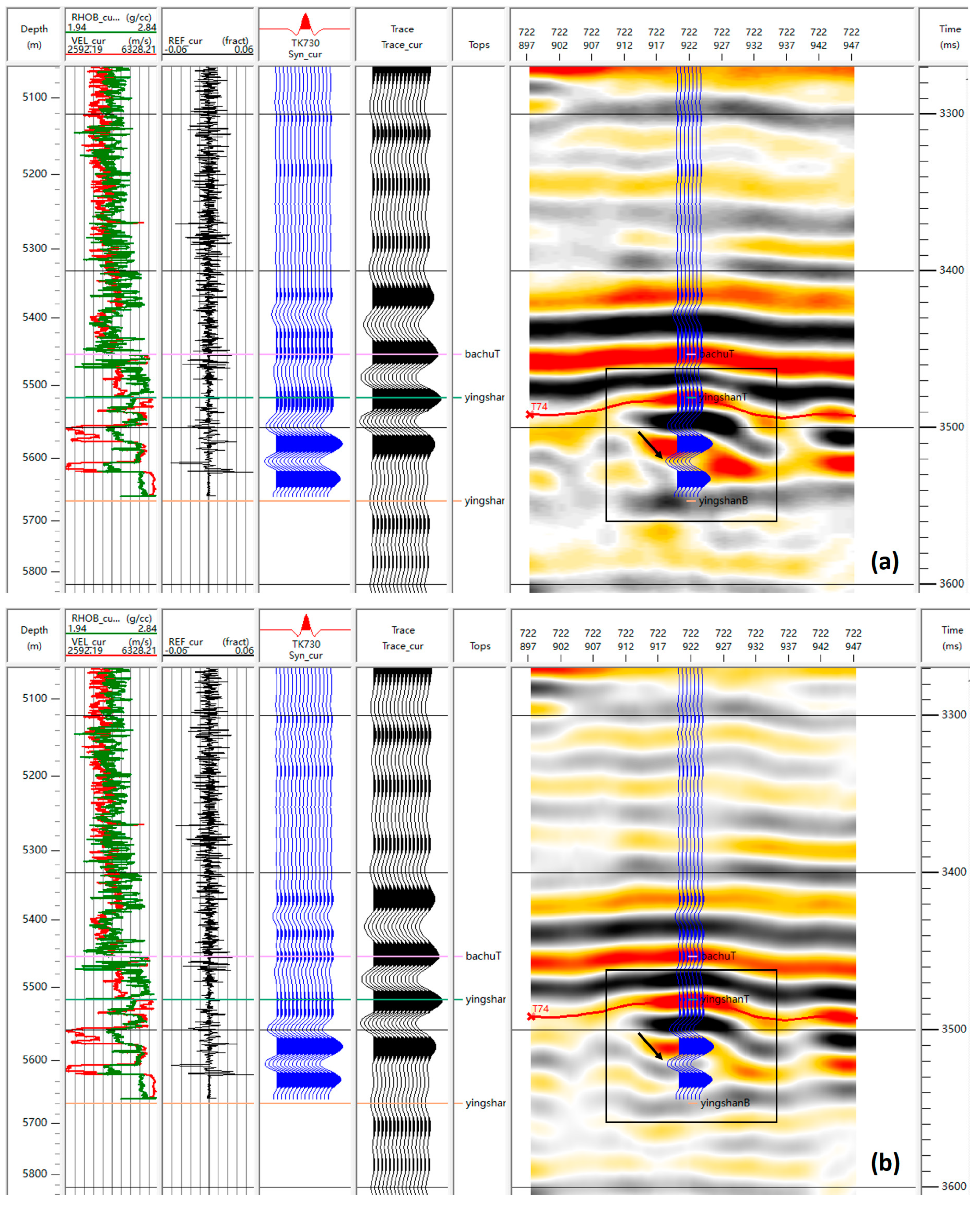
What we are attempting to investigate here is whether the single-frequency data selected in the previous section are consistent with the real strata. We select the logging data acoustic velocity (AC) and lithological density (DEN) of 10 wells to synthesize the seismic traces, which are compared to the single-frequency traces around the wells. The wavelet selected is the Ricker wavelet, the main frequency of which refers to the main frequency of the seismic data around the well. The synthetic traces with a Ricker Wavelet of 30 Hz as the dominant frequency and synthetic traces with a Ricker Wavelet of 35 Hz as the dominant frequency are shown in blue color in Figure 6a,b, respectively.

The results from Figure 6 reveal that, in the black square frame, the well-side seismic traces in Figure 6b are highly consistent with the synthetic traces (look at the black arrow), and the caves (“bead” shape) in the target layer are distinguishable. The well-side seismic traces in Figure 6a are less consistent with the synthetic traces (look at the black arrow), the “beads” are not easy to distinguish, and the lateral continuity is poor. In terms of priority illumination, seismic events of the reservoir are preferentially illuminated by certain frequency components [49]. This well-constrained result further verifies that the 35 Hz single-frequency data volume can be used as the real reservoir response to characterize the distribution of the reservoir.

4.3. Characterization of the Reservoir Distribution by a Waveform Cluster

Before applying the waveform cluster method mentioned in Section 3.2, we perform the following two steps to prepare the waveform data. First, we select the seismic data slice within 50 ms below the T74 top (shown by the red horizon in Figure 6) that has been calibrated. Because we know where the gas reservoir is, we do expect to accurately characterize the fracture-cavity paleo-channel reservoir in this data slice. This means that the Carboniferous Bachu Formation overlying the top-bottom of the Middle-Lower Ordovician (T74 top) is leveled to characterize the paleo-geomorphology of the Hercynian period. Second, we normalize the 68,750 ($250\times 275$) waveforms of the seismic data slice.

The following factors should be considered before performing a waveform cluster: (1) when there is calibration of the underlying layers, the calibration of the stratum is suggested to be used as the geological constraint for selecting the time slice window; (2) when selecting the suitable number of typical waveforms, the prior geological understanding of the target layer, the existing well-logging data, and a trial-and-error method should be combined to make the best decision. In this project, we choose three clusters to represent the paleo-channel, the fractured caves, and the rock basis, respectively; (3) the results of the waveform cluster need further geological analysis to obtain more reliable reservoir prediction results.

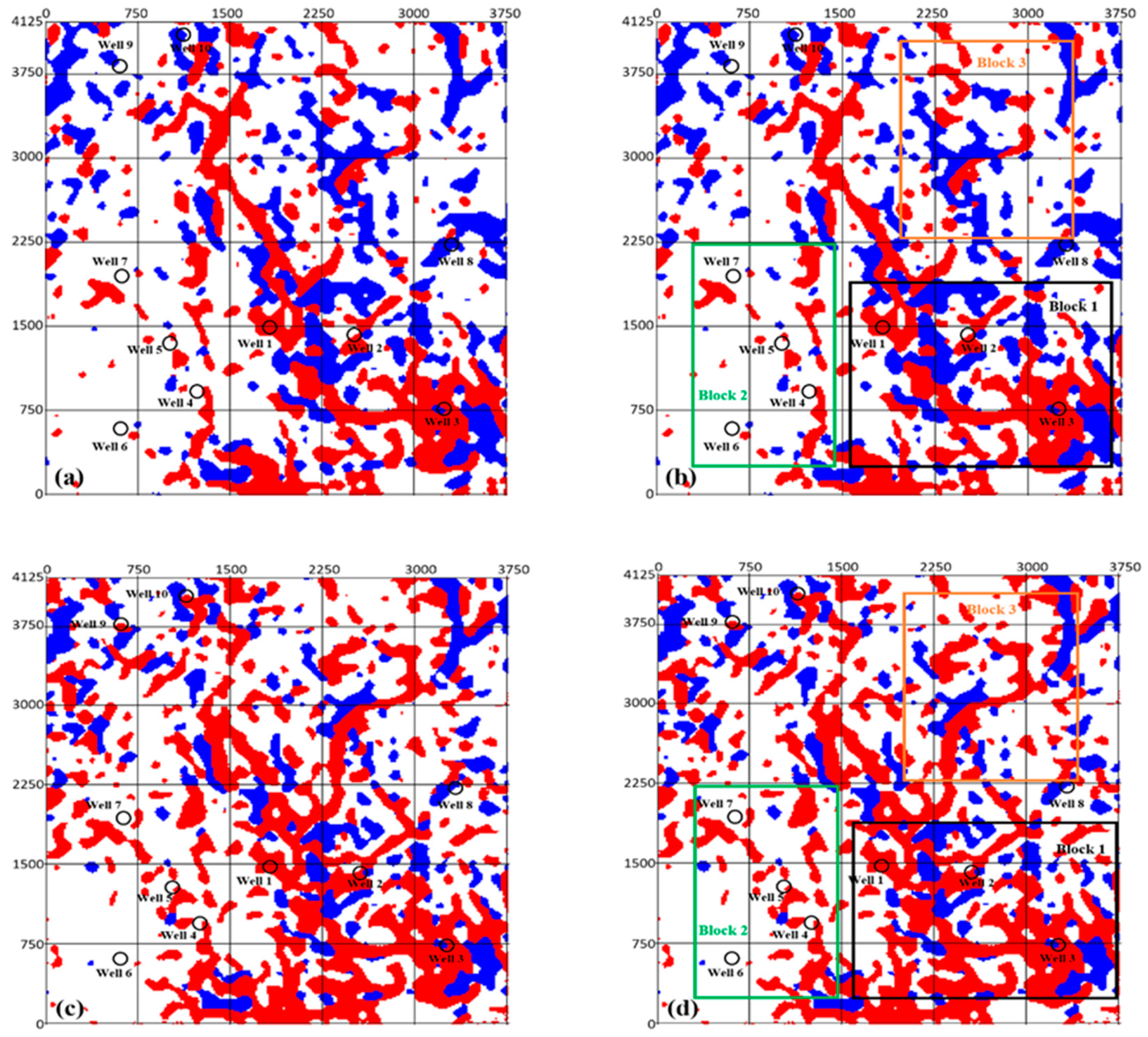
The waveform clustering results (Figure 7) of the Block 7 of the Tahe Oilfield show that the karst paleo-channels of multiple scales and different directions are intertwined with fractured caves of various sizes in the middle-upper depth of the Ordovician. In the north–south direction, a network-like paleo-channel with good connectivity has developed, which has a groove-like structural feature. The main paleo-river channel and branch paleo-river channel are clearly distributed, which is very similar to the modern river channel. The distribution of the surface paleokarst drainage system at the top of the Ordovician is similar to that of modern karst-drainage systems [6]. In the southern part of the study area, channels in the east–west direction have also developed (see black box 1). In the northwest, the channels are not developed, but “bead” shaped caves (shown in blue) are distributed in a scattered manner. The branch to the east side has a length of about 4 km and a width of 100 to 300 m. The length of the branch to the west side is about 3 km and the width is between 80 and 400 m. It can be inferred that the target reservoir has good inner diameter flow conditions with a continuous distribution of soluble rock masses.

Figure 7b,d are the results of waveform clustering on the original data and the 35-Hz frequency data, respectively. Although the results are substantially the same, the clustering results for the 35-Hz frequency data are significantly better than those for the full-band data. Comparing Figure 7b with Figure 7d, it can be seen that, on the 35-Hz frequency data:

(1)

The connectivity between wells is much better, such as the connection between Well 1, Well 2, and Well 3 in Block 1, and Well 4, Well 5, and Well 6 in Block 2. The river connectivity in Block 3 is significantly improved and the river width is widened. Previous studies on the karst development [2,3,14,46,88] and the actual drilling process show that Well 1 and Well 2 have a certain degree of connectivity (Figure 7d), which is not shown in the clustering results of the full-band data (Figure 7b). The near-shore karst platform and gentle karst slopes of the ancient channel were formed by strong hydrodynamic erosion, which can easily form a pipeline system “crossing the mountain”. The pipeline system is less damaged by the filling in the later stage, and the formed oil and gas reservoirs are larger. An increase in the connectivity of the paleo-channel may indicate a corresponding increase in reservoir connectivity.

(2)

The portrayed trend in channels is more obvious. Well 4, Well 5, and Well 7 in Block 2 of Figure 7b are randomly distributed, which suggests that there is no connection between them. The connectivity in Block 2 of Figure 7d is better and the trend in channels is more obvious, which indicate that a small channel branch may have formed. This provides a new perspective for understanding the crack caves in the Tahe Oilfield.

In summary, the 35-Hz frequency seismic data provide us with a better seismic data analysis, a more reliable geological description to understand the history of the reservoir’s formation and development, and more accuracy to predict potential well locations in the area. Other techniques for identifying paleo-channels include three-dimensional visual techniques, integrated interpretation of multiple attributes, including amplitude, and coherent techniques [45,52,72,73].

4.4. Geological and Geophysical Interpretation of the Reservoir

The Paleokarst of the Ordovician in the Tahe Oilfield is in the middle of the Akekule karst slope zone. It has been subjected to atmospheric freshwater dissolution for long periods, has a long exposure time, and has undergone multi-stage karst and tectonic movement reconstruction. The general characteristics of karst systems have been extensively published, and modern cave systems are well-studied [89,90,91,92,93,94,95]. The distribution of fracture-cavity channel systems formed by the action of paleo-karst water can be divided into network, dendritic, pinnate, single-pipe, individual, and other forms [88]. The karst platforms and gentle karst slopes near the ancient rivers are strongly hydro-dynamically eroded, forming karst landforms with a low degree of late filling and damage, and large reservoirs have formed around the karst landforms. Complex Ordovician oil and gas reservoirs are usually not structural fractures but depend on stratigraphic traps [6].

The connectivity and geological similarity of the ancient river channel can help us to understand the trapping of the reservoir. Therefore, if information on the reservoir’s connectivity can be mined from logging data and seismic data, it will provide us with a new understanding of reservoir prediction. As can be seen from Figure 7d, the main channel accounts for the largest part of the total volume of the region, which is about 55.3%. Branch channels account for 28.94%, indicating that branch channels are also important for oil and gas exploration. The more obvious trend of the branch channel in Figure 7d indicates that the “beads” (fractured caves) near the channels of Block 2 and Block 3 may be favorable Carbonate fracture-cavity reservoirs.

Carbonate fractures usually contain fluids (oil, gas, or water), causing a decrease in the seismic reflection frequency. However, sometimes, the reflection frequency may increase when the reservoir consists of a series of small holes and cracks. This is mainly because the scattered or diffracted waves generated by a series of small cracks and caves are superimposed on each other, causing the main frequency to rise. In fact, the amplitude component of a certain frequency associated with a cracked cave is still weakened [6]. Fractured-cavity reservoirs, on the other hand, are typically relatively thin. It is known from the tuning characteristics of the thin layer [37] and the characteristics of the low-pass frequency filtering that the reflection of the fracture-caves has a strong amplitude and the amplitude corresponding to a certain high-frequency component varies. Therefore, the time-frequency characteristics corresponding to a specific frequency can be used to predict the distribution of carbonate reservoirs. The sharpness of geological phenomena in different frequency data is significantly different. Our selection of reservoir-sensitive single-frequency data may be related to thin-layer tuning effects, which are not elaborated on in detail here due to constraints on the article’s length. For articles on the tuning characteristics of the thin layer, see [37,52,96].

5. Conclusions

The Ordovician carbonate strata in the Tahe oilfield are deeply buried. The irregular geometry and the associated extreme heterogeneity, when combined with the weak quality of the seismic data, make it difficult to accurately predict the distribution of reservoirs using the traditional full-band seismic data. We use Matching Pursuit and well-log data as geological constraints to extract the reservoir-sensitive single-frequency data, which are then used by a Waveform Cluster to characterize the reservoir distribution. The method is applied to an area in the Tahe Oilfield. The results show that the method can describe the distribution of fracture-cavity paleo-channel reservoirs more reliably. This indicates that the method is promising and can effectively guide oil and gas exploration in the Tahe Oilfield and other similar karstic groundwater and karst hydrogeological systems.

References

- Zhu, G.; Zhang, B.; Yang, H.; Su, J.; Liu, K.; Zhu, Y. Secondary alteration to ancient oil reservoirs by late gas filling in the Tazhong area, Tarim Basin. J. Pet. Sci. Eng. 2014, 122, 240–256. [Google Scholar] [CrossRef]
- Tian, F.; Jin, Q.; Lu, X.; Lei, Y.; Zhang, L.; Zheng, S.; Zhang, H.; Rong, Y.; Liu, N. Multi-layered ordovician paleokarst reservoir detection and spatial delineation: A case study in the Tahe Oilfield, Tarim Basin, Western China. Mar. Pet. Geol. 2016, 69, 53–73. [Google Scholar] [CrossRef]
- Tian, F.; Lu, X.; Zheng, S.; Zhang, H.; Rong, Y.; Yang, D.; Liu, N. Structure and filling characteristics of paleokarst reservoirs in the Northern Tarim basin, revealed by outcrop, core and borehole images. Open Geosci. 2017, 9, 266–280. [Google Scholar] [CrossRef]
- Zhang, B.; Liu, J. Classification and characteristics of karst reservoirs in china and related theories. Pet. Explor. Dev. 2009, 36, 12–29. [Google Scholar] [CrossRef]
- Yang, H.; Xue, F.; Pan, W.; Chen, L.; Yang, P.; Tong, Y. Seismic description of karst topography and caves of Ordovician carbonate reservoirs, Lungu area, Tarim Basin, West China. In SEG Technical Program Expanded Abstract 2010; Society of Exploration Geophysicists: Tulsa, OK, USA, 2010; pp. 1256–1260. [Google Scholar] [CrossRef]
- Zeng, H.; Loucks, R.; Janson, X.; Wang, G.; Xia, Y.; Yuan, B.; Xu, L. Three-dimensional seismic geomorphology and analysis of the Ordovician paleokarst drainage system in the central Taber Uplift, northern Tarim Basin, western China. AAPG Bull. 2011, 95, 2061–2083. [Google Scholar] [CrossRef]
- Dou, Q.; Sun, Y.; Sullivan, C.; Guo, H. Paleokarst system development in the san andres formation, permian basin, revealed by seismic characterization. J. Appl. Geophys. 2011, 75, 379–389. [Google Scholar] [CrossRef]
- Li, Y.; Zheng, X.; Zhang, Y. High-frequency anomalies in carbonate reservoir characterization using spectral decomposition. Geophysics 2011, 76, v47–v57. [Google Scholar] [CrossRef]
- Taherdangkoo, R.; Abdideh, M. Application of wavelet transform to detect fractured zones using conventional well logs data (Case study: Southwest of Iran). Int. J. Pet. Eng. 2016, 2, 125. [Google Scholar] [CrossRef]
- Li, F.; Lu, W. Coherence attribute at different spectral scales. Interpretation 2014, 2, SA99–SA106. [Google Scholar] [CrossRef]
- Li, C.; Gao, Y.; Zhang, H.; Wang, H. Identification of small-scale carbonate reservoir. In Proceedings of the CPS/SEG Beijing International Geophysical Conference, Beijing, China, 21–24 April 2014. [Google Scholar]
- Parchkoohi, M.H.; Farajkhah, N.K.; Delshad, M.S. Automatic detection of karstic sinkholes in seismic 3d images using circular hough transform. J. Geophys. Eng. 2015, 12, 764–769. [Google Scholar] [CrossRef]
- Liu, Y.; Wang, Y. Case History Seismic characterization of a carbonate reservoir in Tarim Basin. Geophysics 2017, 82, b177–b188. [Google Scholar] [CrossRef]
- Lu, X.; Wang, Y.; Tian, F.; Li, X.; Yang, D.; Li, T.; Lv, Y.; He, X. New insights into the carbonate karstic fault system and reservoir formation in the Southern Tahe area of the Tarim Basin. Mar. Pet. Geol. 2017, 86, 587–605. [Google Scholar] [CrossRef]
- Taherdangkoo, R.; Abdideh, M. Fracture density estimation from well logs data using regression analysis: Validation based on image logs (Case study: South West Iran). Int. J. Pet. Eng. 2016, 2, 289. [Google Scholar] [CrossRef]
- Liu, Y.; Hou, J.; Li, Y.; Dong, Y.; Ma, X.; Wang, X. Characterization of architectural elements of ordovician fractured-cavernous carbonate reservoirs, Tahe Oilfield, China. J. Geol. Soc. India 2018, 91, 315–322. [Google Scholar] [CrossRef]
- Zhang, T.; Yan, X.B. A study of the genetics of karst-type subtle reservoir in Tahe oilfield. Petrol. Sci. 2004, 2, 99–104, (In Chinese with English Abstract). [Google Scholar]
- He, Z.L.; Peng, S.T.; Zhang, T. Controlling factors and genetic pattern of the Ordovician reservoirs in the Tahe area, Tarim Basin. Oil Gas Geol. 2010, 31, 743–752, (In Chinese with English Abstract). [Google Scholar]
- Huang, D.; Liu, Z.; Wang, W. Evaluating the impaction of coal mining on Ordovician KarstWater through statistical methods. Water 2018, 10, 1409. [Google Scholar] [CrossRef]
- Zhu, G.; Zhang, S.; Su, J.; Zhang, B.; Yang, H.; Zhu, Y.; Gu, L. Alteration and multi-stage accumulation of oil and gas in the Ordovician of the Tabei Uplift, Tarim Basin, NW China: Implications for genetic origin of the diverse hydrocarbons. Mar. Pet. Geol. 2013, 48, 111–112. [Google Scholar] [CrossRef]
- Dou, Z.L. Description and reserves calculation of fractured-vuggy carbonate reservoirs. Pet. Geol. Exp. 2014, 36, 9–15, (In Chinese with English Abstract). [Google Scholar]
- Meng, M.; Fan, T.; Yin, S.; Gao, Z.; Jiang, L.; Yu, C.; Jiang, L. Characterization of carbonate microfacies and reservoir pore types based on formation microImager logging: A case study from the Ordovician in the Tahe Oilfield, Tarim Basin, China. Interpretation 2017, 6, T71–T82. [Google Scholar] [CrossRef]
- Tian, F.; Di, Q.; Jin, Q.; Cheng, F.; Zhang, W.; Lin, L.; Wang, Y.; Yang, D.; Niu, C.; Li, Y. Multiscale Geological-Geophysical Characterization of the Epigenic Origin and Deeply Buried Paleokarst System in Tahe Oilfield, Tarim Basin. Mar. Pet. Geol. 2019, 102, 16–32. [Google Scholar] [CrossRef]
- Chen, Z.; Deng, Y.; Xu, B.; Dong, J. Bottom water breakthrough prediction in fractured-vuggy reservoirs with bottom water-an example from the well s48 in block 4 of Tahe oilfield. Oil Gas Geol. 2012, 33, 791–795. [Google Scholar] [CrossRef]
- Li, C.; Wang, X.; Li, B.; He, D. Paleozoic fault systems of the Tazhong uplift, Tarim basin, China. Mar. Pet. Geol. 2013, 39, 48–58. [Google Scholar] [CrossRef]
- Yun, L.; Cao, Z. Hydrocarbon enrichment pattern and exploration potential of the ordovician in Shunnan area, Tarim basin. Oil Gas Geol. 2014, 35, 788–797, (In Chinese with English Abstract). [Google Scholar]
- Qi, L.X.; Gu, H.; Li, Z.M.; Lu, X.B. Theoretical discussion on resolution of maximum height of cavity in the Tahe oil field based on seismic amplitude. Prog. Geophys. 2008, 23, 1499–1506, (In Chinese with English Abstract). [Google Scholar]
- Sun, S.Z.; Zhou, X.; Yang, H.; Wang, Y.; Wang, D.; Liu, Z. Fractured reservoir modeling by discrete fracture network and seismic modeling in the Tarim basin, China. Pet. Sci. 2011, 8, 433–445. [Google Scholar] [CrossRef]
- Jin, Q.; Tian, F. Investigation of fracture-cavity constructions of Ordovician karst reservoirs in the Tahe Oilfield, Tarim Basin, Western China. J. China Univ. Pet. 2013, 37, 15–21, (In Chinese with English Abstract). [Google Scholar]
- Yue, P.; Xie, Z.; Liu, H.; Chen, X.; Guo, Z. Application of water injection curves for the dynamic analysis of fractured-vuggy carbonate reservoirs. J. Petrol. Sci. Eng. 2018, 169, 220–229. [Google Scholar] [CrossRef]
- Li, K.; Cai, C.; Cai, L.; Jiang, L.; Xiang, L. Origin of sulfides in the middle and lower ordovician carbonates in Tahe oilfield, Tarim basin. Acta Petrol. Sin. 2012, 28, 806–814. [Google Scholar] [CrossRef]
- Kerans, C. Karst-controlled reservoir heterogeneity in Ellenburger group carbonates of west Texas. AAPG Bull. 1988, 72, 1160–1183. [Google Scholar] [CrossRef]
- Jia, C.; Pang, X. Research processes and main development directions of deep hydrocarbon geological theories. Acta Pet. Sin. 2015, 36, 1457–1469. [Google Scholar] [CrossRef]
- Kuang, L.; Guo, J.; Huang, T. Forming mechanism of hydrocarbon reservoirs in Yingshan Formation of Yuqi block in Akekule arch, Tarim Basin. J. Cent. South Univ. Technol. 2008, 15, 244–250, (In Chinese with English Abstract). [Google Scholar] [CrossRef]
- Liu, C.Y.; Lin, C.S.; Wang, Y.; Wang, M.B. Burial dissolution of Ordovician granule limestone in the Tahe Oilfield of the Tarim Basin, NW China, and its geological significance. Acta Geol. Sin. Engl. Ed. 2008, 82, 520–529. [Google Scholar] [CrossRef]
- Morlet, J.; Arens, G.; Fourgeau, E.; Giard, D. Wave propagation and sampling theory—Part II: Sampling theory and complex waves. Geophysics 1982, 47, 222–236. [Google Scholar] [CrossRef]
- Partyka, G.; Gridley, J.; Lopez, J. Interpretational applications of spectral decomposition in reservoir characterization. Lead. Edge 1999, 18, 353–360. [Google Scholar] [CrossRef]
- Chopra, S.; Marfurt, K.J. Seismic Attributes for Prospect Identification and Reservoir Characterization; Society of Exploration Geophysicists: Tulsa, OK, USA, 2007; ISBN 978-1-56080-141-2. [Google Scholar]
- Meza, R.; Sierra, A.; Castaqna, J.; Barbato, U. Joint time-variant spectral analysis, part II: A case study. Interpretation 2018, 6, T985–T999. [Google Scholar] [CrossRef]
- Chakraborty, A.; Okaya, D. Frequency-time decomposition of seismic data using wavelet-based methods. Geophysics 1995, 60, 1906–1916. [Google Scholar] [CrossRef]
- Castagna, J.; Oyem, A.; Portniaguine, O.; Aikulola, U. Phase decomposition. Interpretation 2016, 4, SN1–SN10. [Google Scholar] [CrossRef]
- Wang, X.; Zhang, B.; Li, F.; Qi, J.; Bai, B. Seismic time-frequency decomposition by using a hybrid basis-matching pursuit technique. Interpretation 2016, 4, T239–T248. [Google Scholar] [CrossRef]
- Lu, W.; Li, F. Seismic spectral decomposition using deconvolutive short-time Fourier transform spectrogram. Geophysics 2013, 78, V43–V51. [Google Scholar] [CrossRef]
- Sinha, S.; Routh, P.S.; Anno, P.D.; Castagna, J.P. Spectral decomposition of seismic data with continuous-wavelet transform. Geophysics 2005, 70, P19–P25. [Google Scholar] [CrossRef]
- Matos, M.C.; Davogustto, O.; Zhang, K.; Marfurt, K.J. Detecting stratigraphic discontinuities using time-frequency seismic phase residues. Geophysics 2011, 76, P1–P10. [Google Scholar] [CrossRef]
- Tian, F.; Chen, S.; Zhang, E.; Gao, J.; Chen, W.; Zhang, Z.; Li, Y. Generalized S transform and its applications for analysis of seismic thin beds. In SEG Technical Program Expanded Abstract 2002; Society of Exploration Geophysicists: Tulsa, OK, USA, 2002; pp. 2217–2220. [Google Scholar] [CrossRef]
- Ruthner, M.P.; Oliveira, A.S. Application of S transform in the spectral decomposition of seismic data. In Proceedings of the 9th International Congress of the Brazilian Geophysical Society & EXPOGEF, Salvador, Bahia, Brazil, 11–14 September 2005. [Google Scholar]
- Wu, L.; Castagna, J. S-transform and Fourier transform frequency spectra of broadband seismic signals. Geophysics 2017, 82, O71–O81. [Google Scholar] [CrossRef]
- Castagna, J.P.; Sun, S.; Siegfried, R.W. Instantaneous spectral analysis: Detection of low-frequency shadows associated with hydrocarbons. Lead. Edge 2003, 22, 120–127. [Google Scholar] [CrossRef]
- Puryear, C.I.; Portniaguine, O.N.; Cobos, C.M.; Castagna, J.P. Constrained least-squares spectral analysis: Application to seismic data. In SEG Technical Program Expanded Abstract 2012; Society of Exploration Geophysicists: Tulsa, OK, USA, 2012; pp. 1–5. [Google Scholar] [CrossRef]
- Peyton, L.; Bottjer, R.; Partyka, G. Interpretation of incised valleys using new 3-D seismic techniques: A case history using spectral decomposition and coherency. Lead. Edge 1998, 17, 1294–1298. [Google Scholar] [CrossRef]
- Marfurt, K.J.; Kirlin, R.L. Narrow-band spectral analysis and thin-bed tuning. Geophysics 1999, 66, 1274–1283. [Google Scholar] [CrossRef]
- Wang, Y. Seismic time-frequency spectral decomposition by matching pursuit. Geophysics 2007, 72, v13–v20. [Google Scholar] [CrossRef]
- Mallat, S. A Wavelet Tour of Signal Processing, Third Edition: The Sparse Way, 3rd ed.; Academic Press: Orlando, FL, USA, 2008; ISBN1 0123743702. ISBN2 9780123743701. [Google Scholar]
- Rioul, O.; Vetterli, M. Wavelets and Signal Processing. IEEE Signal Process. Mag. 1991, 8, 14–38. [Google Scholar] [CrossRef]
- Hlawatsch, F.; Boudreauxbartels, G.F. Linear and quadratic time-frequency signal representations. IEEE Signal Process. Mag. 1992, 9, 21–67. [Google Scholar] [CrossRef]
- Abry, P.; Gonçalvès, P.; Flandrin, P. Wavelet-based spectral analysis of 1/f processes. In Proceedings of the 1993 IEEE International Conference on Acoustics, Speech, and Signal Processing, Minneapolis, MN, USA, 27–30 April 1993. [Google Scholar]
- Stockwell, R.G.; Mansinha, L.; Lowe, R.P. Localization of the complex spectrum: The S transform. IEEE Trans. Signal Process. 2002, 44, 998–1001. [Google Scholar] [CrossRef]
- Mallat, S.G.; Zhang, Z. Matching pursuits with time-frequency dictionaries. IEEE Trans Signal Process. 1993, 41, 3397–3415. [Google Scholar] [CrossRef]
- Rojas, N.; Davis, T.L. Spectral Decomposition applied to time-lapse seismic interpretation, Rulison Field, Colorado. In SEG Technical Program Expanded Abstract 2009; Society of Exploration Geophysicists: Tulsa, OK, USA, 2009; pp. 3845–3849. [Google Scholar] [CrossRef]
- Qian, S.; Chen, D. Signal representation using adaptive normalized gaussian functions. Signal Process. 1994, 36, 1–11. [Google Scholar] [CrossRef]
- Rebollo-Neira, L.; Lowe, D. Optimized orthogonal matching pursuit approach. IEEE Signal Process. Lett. 2002, 9, 137–140. [Google Scholar] [CrossRef]
- Capobianco, E. Independent multiresolution component analysis and matching pursuit. Comput. Stat. Data Anal. 2003, 42, 385–402. [Google Scholar] [CrossRef]
- Andrle, M.; Rebollo-Neira, L. A swapping-based refinement of orthogonal matching pursuit strategies. Signal Process. 2006, 86, 480–495. [Google Scholar] [CrossRef]
- Andrle, M.; Rebollo-Neira, L.; Sagianos, E. Backward-Optimized Orthogonal Matching Pursuit Approach. IEEE Signal Process. Lett. 2004, 11, 705–708. [Google Scholar] [CrossRef]
- Castagna, J.P.; Sun, S. Comparison of spectral decomposition methods. First Break 2006, 24, 75–79. [Google Scholar]
- Djeffal, A. Enhancement of Margrave Deconvolution and Qestimation in Highly Attenuating Media Using the Modified S-Transform. Master’s Thesis, Michigan Technological University, Houghton, MI, USA, 2016. [Google Scholar]
- Pinnegar, C.R.; Mansinha, L. The S-transform with windows of arbitrary and varying shape. Geophysics 2003, 68, 381–385. [Google Scholar] [CrossRef]
- Pinnegar, C.R.; Eaton, D.W. Application of the s transform to prestack noise attenuation filtering. J. Geophys. Res. Solid Earth 2003, 108, 2422–2431. [Google Scholar] [CrossRef]
- Nguyen, T.; Castagna, J. Matching Pursuit of Two Dimensional Seismic Data and Its Filtering Application. In SEG Technical Program Expanded Abstract 2000; Society of Exploration Geophysicists: Tulsa, OK, USA, 2000; pp. 2067–2069. [Google Scholar] [CrossRef]
- Liu, J.; Wu, Y.; Li, X. Time-Frequency decomposition based on Ricker wavelet. In SEG Technical Program Expanded Abstract 2004; Society of Exploration Geophysicists: Tulsa, OK, USA, 2004; pp. 1937–1940. [Google Scholar] [CrossRef]
- Liu, J.; Marfurt, K.J. Matching pursuit decomposition using Morlet wavelets. In SEG Technical Program Expanded Abstract 2005; Society of Exploration Geophysicists: Tulsa, OK, USA, 2005; pp. 786–789. [Google Scholar] [CrossRef]
- Liu, J.; Marfurt, K.J. Instantaneous spectral attributes to detect channels. Geophysics 2007, 72, p23–p31. [Google Scholar] [CrossRef]
- Wang, Y. Multichannel matching pursuit for seismic trace decomposition. Geophysics 2010, 75, V61–V66. [Google Scholar] [CrossRef]
- Wen, X.; Zhang, B.; Pennington, W.; He, Z. Relative P-impedance estimation using a dipole-based matching pursuit decomposition strategy. Interpretation 2015, 3, T197–T206. [Google Scholar] [CrossRef]
- Arshin, B.M.; Ghazali, A.R.; Amin, Y.K.; Barnes, A.E. Hybrid Waveform Classification Applied to Delineate Compartments in a Complex Reservoir in the Malay Basin. In Proceedings of the International Petroleum Technology Conference, Kuala Lumpur, Malaysia, 10–12 December 2014. [Google Scholar]
- Basman, Y.V. Seismic waveform classification renewing the interest in Barrolka field, SW Queensland, Cooper Basin. In Proceedings of the ASEG Extended Abstracts 2015: 24th International Geophysical Conference and Exhibition, Perth, Australia, 15–18 February 2015; pp. 1–3. [Google Scholar]
- John, A.K.; Lake, L.W.; Torresverdin, C.; Srinivasan, S. Seismic facies identification and classification using simple statistics. SPE Reserv. Eval. Eng. 2008, 11, 984–990. [Google Scholar] [CrossRef]
- Roy, A.; Matos, M.; Marfurt, K.J. Automatic Seismic Facies Classification with Kohonen Self Organizing Maps—A Tutorial. Geohorizons J. Soc. Pet. Geophys. 2010, 6–14. [Google Scholar]
- Zeng, H. Seismic geomorphology-based facies classification. Lead. Edge 2004, 23, 644–688. [Google Scholar] [CrossRef]
- Ross, C.P.; Cole, D.M. A Comparison of Popular Neural Network Facies-Classification Schemes. Lead. Edge 2017, 36, 340–349. [Google Scholar] [CrossRef]
- Huang, K.-Y.; Weng, L.-S.; University, N.C.T.; Shen, L.-C. Well Log Data Inversion Using Radial Basis Function Network. In Proceedings of the 2011 IEEE International Geoscience and Remote Sensing Symposium, Vancouver, BC, Canada, 24–29 July 2011; Volume 5. [Google Scholar]
- Li, K.; She, B.; Liu, Z.; Su, M.; Hu, G. Supervised Seismic Facies Analysis Using Discrimination Dictionary. In SEG Technical Program Expanded Abstracts 2018; Society of Exploration Geophysicists: Anaheim, CA, USA, 2018; pp. 1585–1589. [Google Scholar]
- Huang, K.-Y.; Hsieh, W.-H. Cellular Neural Network for Seismic-Pattern Recognition. In SEG Technical Program Expanded Abstracts 2018; Society of Exploration Geophysicists: Anaheim, CA, USA, 2018; pp. 2221–2225. [Google Scholar]
- Taherdangkoo, R.; Taherdangkoo, M. Modified Stem Cells Algorithm-Based Neural Network Applied to Bottom Hole Circulating Pressure in Underbalanced Drilling. Int. J. Pet. Eng. 2015, 1, 178. [Google Scholar] [CrossRef]
- Halkidi, M.; Batistakis, Y.; Vazirgiannis, M. On clustering validation techniques. J. Intell. Inf. Syst. 2001, 17, 107–145. [Google Scholar] [CrossRef]
- Xu, R.; Wunsch, D. Survey of Clustering Algorithms. IEEE Trans. Neural Netw. 2005, 16, 645–678. [Google Scholar] [CrossRef]
- Tian, F.; Luo, X.; Zhang, W. Integrated Geological-Geophysical Characterizations of Deeply Buried Fractured-Vuggy Carbonate Reservoirs in Ordovician Strata, Tarim Basin. Mar. Pet. Geol. 2019, 99, 292–309. [Google Scholar] [CrossRef]
- Liu, W.; Zhang, L.; Liu, P.; Qin, X.; Shan, X.; Yao, X. FDOM conversion in karst watersheds expressed by three-dimensional fluorescence spectroscopy. Water 2018, 10, 1427. [Google Scholar] [CrossRef]
- Palmer, A.N. Origin and Morphology of Limestone Caves. Geol. Soc. Am. Bull. 1991, 103, 1–21. [Google Scholar] [CrossRef]
- Jebreen, H.; Banning, A.; Wohnlich, S.; Niedermayr, A.; Ghanem, M.; Wisotzky, F. The Influence of Karst Aquifer Mineralogy and Geochemistry on Groundwater Characteristics: West Bank, Palestine. Water 2018, 10, 1829. [Google Scholar] [CrossRef]
- Malenica, L.; Gotovac, H.; Kamber, G.; Simunovic, S.; Allu, S.; Divic, V. Groundwater Flow Modeling in Karst Aquifers: Coupling 3D Matrix and 1D Conduit Flow via Control Volume Isogeometric Analysis—Experimental Verification with a 3D Physical Model. Water 2018, 10, 1787. [Google Scholar] [CrossRef]
- Zhang, Z.; Wang, W.; Qu, S.; Huang, Q.; Liu, S.; Xu, Q.; Ni, L. A New Perspective to Explore the Hydraulic Connectivity of Karst Aquifer System in Jinan Spring Catchment, China. Water 2018, 10, 1368. [Google Scholar] [CrossRef]
- Yang, W.; Fang, Z.; Yang, X.; Shi, S.; Wang, J.; Wang, H.; Bu, L.; Li, L.; Zhou, Z.; Li, X. Experimental Study of Influence of Karst Aquifer on the Law of Water Inrush in Tunnels. Water 2018, 10, 1211. [Google Scholar] [CrossRef]
- Ford, D. Characteristics of Dissolutional Cave Systems in Carbonate Rocks. In Paleokarst; James, N.P., Choquette, P.W., Eds.; Springer: New York, NY, USA, 1988; pp. 25–57. [Google Scholar]
- Stark, T.J. Instantaneous Frequency Spectra. Lead. Edge 2015, 34, 72–78. [Google Scholar] [CrossRef]
Figure 1.
The location of the study area and an overview map of the Tarim Basin. (a) Tectonic components of the Tarim Basin, including three uplifts and four depressions with east–west orientations (modified from [17]). The Tahe oilfield is located in the Northern Uplift of the Tarim Basin. (b) The study area is in the center of the Tahe oilfield, which is located in the southwestern part of the Akekule Arch in the Northern Uplift of the Tarim Basin (modified from [18]). (c) Cross Section A-A’, showing the paleokarst system of the Tahe Oilfield. The main reservoirs are located in the northern part of the Tahe Oilfield in the Yingshan Formation (O1–2 years), which is at depths exceeding 5500 m (modified from [2]). See Figure 1b for the cross-section location.
Figure 2.
A flow chart of Matching Pursuit.
Figure 3.
The comparison of time-frequency spectra of a synthetic seismic trace. From left to right, the method used is (a) Continuous Wavelet Transform (CWT), (b) S-Transform (ST), and (c) Matching Pursuit (MP), respectively.
Figure 4.
A flow chart of the fuzzy C-means cluster.
Figure 5.
Seismic sections of different single-frequency data around Well 1. (a)–(d) represent 15 Hz, 20 Hz, 25 Hz, and 30 Hz, respectively. (e) represents 35 Hz. (f)–(h) represent 40 Hz, 45 Hz, 50 Hz, and 55 Hz, respectively. (i) represents the original full-band seismic section.
Figure 6.
A comparison of synthetic traces (blue) with (a) the full-band and (b) a selected 35-Hz frequency profile.
Figure 7.
A comparison of the reservoir distribution by the 35 Hz single-frequency data and the full-band data. (a) and (c) are the direct results of the waveform cluster, while (b) and (d) are the interpretation of the cluster results. (a) and (b) are the full-band data, while (c) and (d) are the 35 Hz single-frequency data.
© 2019 by the authors. Licensee MDPI, Basel, Switzerland. This article is an open access article distributed under the terms and conditions of the Creative Commons Attribution (CC BY) license (http://creativecommons.org/licenses/by/4.0/).
Share and Cite
MDPI and ACS Style
Shan, X.; Tian, F.; Cheng, F.; Yang, C.; Xin, W. Spectral Decomposition and a Waveform Cluster to Characterize Strongly Heterogeneous Paleokarst Reservoirs in the Tarim Basin, China. Water 2019, 11, 256. https://doi.org/10.3390/w11020256
AMA Style
Shan X, Tian F, Cheng F, Yang C, Xin W. Spectral Decomposition and a Waveform Cluster to Characterize Strongly Heterogeneous Paleokarst Reservoirs in the Tarim Basin, China. Water. 2019; 11(2):256. https://doi.org/10.3390/w11020256
Chicago/Turabian StyleShan, Xiaocai, Fei Tian, Fuqi Cheng, Changchun Yang, and Wei Xin. 2019. "Spectral Decomposition and a Waveform Cluster to Characterize Strongly Heterogeneous Paleokarst Reservoirs in the Tarim Basin, China" Water 11, no. 2: 256. https://doi.org/10.3390/w11020256
Note that from the first issue of 2016, this journal uses article numbers instead of page numbers. See further details here.