Comparison of Hydrodynamics Simulated by 1D, 2D and 3D Models Focusing on Bed Shear Stresses


1
Christian Doppler Laboratory for Sediment Research and Management, Institute of Hydraulic Engineering and River Research, Department of Water-Atmosphere-Environment, University of Natural Resources and Life Sciences, Muthgasse 107, A-1190 Vienna, Austria
2
Institute of Hydraulic Engineering and River Research, Department of Water-Atmosphere-Environment, University of Natural Resources and Life Sciences, Muthgasse 107, A-1190 Vienna, Austria
*
Author to whom correspondence should be addressed.
Water 2019, 11(2), 226; https://doi.org/10.3390/w11020226
Submission received: 20 December 2018
/
Revised: 25 January 2019
/
Accepted: 26 January 2019
/
Published: 29 January 2019
(This article belongs to the Special Issue The Application of Hydraulic and Sediment Transport Models in Fluvial Geomorphology)
Abstract
:For centuries, scientists have been attempting to map complex hydraulic processes to empirical formulas using different flow resistance definitions, which are further applied in numerical models. Now questions arise as to how consistent the simulated results are between the model dimensions and what influence different morphologies and flow conditions have. For this reason, 1D, 2D and 3D simulations were performed and compared with each other in three study areas with up to three different discharges. A standardized, relative comparison of the models shows that after successful calibration at measured water levels, the associated 2D/1D and 3D/1D ratios are almost unity, while bed shear stresses in the 3D models are only about 62–86% of the simulated 1D values and 90–100% in the case of 2D/1D. Reasons for this can be found in different roughness definitions, in simplified geometries, in different calculation approaches, as well as in influences of the turbulence closure. Moreover, decreasing 3D/1D ratios of shear stresses were found with increasing discharges and with increasing slopes, while the equivalent 2D/1D ratios remain almost unchanged. The findings of this study should be taken into account, particularly in subsequent sediment transport simulations, as these calculations are often based on shear stresses.

1. Introduction
The interaction between gravity and flow resistance is the mechanism underlying both fundamental hydraulic processes and river morphological changes [1,2].
Following Powell [2], flow resistance is composed of the boundary resistance, vegetation resistance [3,4,5,6,7], channel resistance [8,9,10,11,12], spill resistance [13,14,15,16,17,18] and sediment transport resistance [19,20,21,22,23,24,25] and affects bed shear stress and energy dissipation. The challenge in river hydraulics is to achieve the complexity of flow resistance through physical relationships and engineering approaches to gain knowledge about flow velocities, water depths, bed shear stresses and energy losses in channels [2].
Classical approaches for the calculation of flow variables under the influence of flow resistance are the equations of Darcy–Weisbach, Chezy and Manning–Strickler [26,27,28]. These are empirical methods, which were developed from observations in channels in which the flow resistance was determined almost exclusively from the boundary of the flow—much like a block sliding down a plane [29]. Attempts for modifications of these classical approaches are particularly found for relatively rough beds in numerous subsequent research works [7,25,30,31,32,33,34,35,36,37]. However, the Manning–Strickler equation and the related bed roughness values of Manning’s and Strickler’s are still used in engineering practice and particularly in numerical modelling.
For the determination of the bed roughness value, , Strickler [38] developed an equation considering the grain size distribution of the bed material. On the basis of this investigation Meyer-Peter and Müller [39] as well as Jäggi [40] proposed improved approaches by separately considering the surface layer of the bed material or the variable water depths in the channel, respectively. In addition, guidelines for the determination of -values [41,42,43] have been developed for different channel types. However, the Strickler equation was developed for simplified channel geometries without considering lateral heterogeneities. To address these differences in compound and composite cross sections different approaches were elaborated in various research works [44,45,46,47]. Of particular interest in this context was vegetation in riverine landscape, which has a significant impact on flow resistance [48,49,50].
Despite some uncertainties, including the water depth dependencies of -values, related to the use of Strickler’s value, this approach is employed in a substantial percentage of all numerical simulation studies for the definition of the flow resistance. Most well-known 1D numerical models based on the Saint Venant equations (e.g., HEC-RAS, MIKE 11, etc.) and also 2D numerical models employing the depth-averaged Reynolds-equations (e.g., Hydro_AS-2D, MIKE21, TELEMAC-2D, etc.) define the roughness by Strickler’s or Manning’s value. In contrast, most 3D numerical models (e.g., Delft3D, Fluent, RSim-3D, SSIIM) solving the fully three-dimensional Reynolds-equations with different turbulence closures, typically permit the application of the equivalent sand roughness [51], which is based on the sediment size and also allows accounting for the average height of bed forms. To date, numerous studies [52,53,54,55,56,57,58,59,60,61] have been published based on the mentioned numerical models to calculate hydrodynamic properties and their impacts on rivers.
Moreover, the modelled hydrodynamics are often used for predicting the sediment transport as well as morphological changes in rivers. In this context, the bed shear stress is of particular importance, due to the fact that well-known bed load transport equations [39,62,63,64,65] are based on this variable and are used both in analytical calculations [66,67] as well as numerical simulations [68,69,70,71].
These issues show the paramount importance of roughness values in the calculation of bed shear stresses in the context of numerical simulations. Independent of the dimensionality of the models this roughness value usually represents the main opportunity for parameterizing flow resistance in numerical simulations. Moreover, it is the main variable parameter of choice to achieve successful model calibration implying reasonable difference between measured and modelled water surface elevations as well as flow velocities.
Thus, the central research question of this paper is whether valid calculations of water surface elevations in different model dimensions (1D, 2D and 3D) imply a consistent depiction of flow velocities and near-bed flow forces. Of particular interest is a comparison of simulated bed shear stresses of different models, due to their substantial influence on the simulation of bed load transport. The influence of certain characteristic morphologies including artificial bathymetries, pool-riffle sections as well as river bends is investigated on the basis of three different case studies.
2. Materials and Methods
2.1. Case Studies
The locations of the different case studies are depicted in Figure 1a. Case study 1 (C.1) “S-Shaped Trapezoidal Channel” (Figure 1b) represents controlled conditions within a laboratory experiment and was selected to focus on the influence of river bends without any morphological structures. C.2 “Ybbs” (Figure 1c) was chosen to investigate the effects of a pool-riffle section in a stretched natural river site [72]. The complex morphology of the second natural river site C.3 “Sulm” (Figure 1d) combines the different characteristics representing a river meander with pool-riffle sections [72].
2.1.1. S-Shaped Trapezoidal Channel (C.1)
The laboratory experiment was developed at the Hydraulic Engineering Institute of the University of Innsbruck, consisting of a physical laboratory channel 3.0 m in length followed by two consecutive bends with a mean radius of 4.0 m and apex angle of 60 each, and finally an exit channel being 2.8 m long with a bed slope of 0.005. The banks are sloped by a ratio of 2:3. The bed sediments are characterized by a mean diameter of around 5 mm. One set-up of the physical experiment, with a discharge of 0.09 m3 s−1, was part of the validation study of the numerical model RSim-3D [73], which is also used within this research. Measurements of the water surface elevation gained during the experiment form the basis for calibrating the numerical models.
2.1.2. Ybbs (C.2)
The river site C.2 “Ybbs” (Figure 1c) has a total length of around 300 m with an average bed slope of 0.0055 and is classified as a straight river due to natural morphological constraints [74]. The bed sediments are characterized by a mean diameter of around 70 mm [72], excluding the riffle section (located between cross-section 21 and 31) with a of around 93 mm. The hydrology is defined by conditions during low flow (), mean flow (), and a flood with a return period of one year (). In the course of a monitoring campaign in 2006, the bathymetry as well as the water surface elevation were measured at low flow conditions in a local reference system and are the basis for calibrating the numerical models within this study. The calibrated models are further used in the course of the comparison study including the simulation of and . Due to the fact that the valley margins of C.2 are close to the river bed, the inundation areas are greatly reduced, thus this river site is particularly suitable for a sensitivity analysis of flow resistances during floods.
2.1.3. Sulm (C.3)
The river site C.3 “Sulm” (Figure 1d) has a total length of around 500 m with an average bed slope of 0.0010 and is classified as a meandering river [74] with a mean diameter of the surface layer of around 42 mm [72]. The hydrology is characterized by conditions during low flow (), mean flow () and a flood with a return period of one year (). During a monitoring campaign in 2002, the bathymetry as well as the water surface elevation were measured at low flow conditions and are the basis for calibrating numerical models within this study. Additionally, is simulated with the calibrated models in the course of the comparison study.
2.2. Basic Principles
2.2.1. Empirical Relationship between the Equivalent Sand Roughness ks and the Strickler Value kst
Strickler [38] established the eponymous roughness value considering the grain size distribution of the bed material, which is given by
where is an empirical parameter and is the equivalent sand roughness, which is a characteristic value of the grain size distribution. Following this approach Meyer-Peter and Müller [39] as well as USACE [43] adjusted and (Table 1). According to Table 1, ranges between grain size diameters of and , for which 50% and 90% of the cumulative mass are finer, respectively. Jäggi [40] retained the fundamental concept of Strickler, whereby he developed a new approach for calculating
which depends on the relative roughness —including and the water depth —and the bed slope , resulting in a range of possible values (Table 1).
2.2.2. Calculation of Bed Shear Stress
Before going into the details of any results, the numerical principles of bed shear stress calculations in different models are demonstrated. The classical approach in hydraulic engineering for determining the average bed shear stress in a cross-section is known as the Du Boys equation and is given by
where is the density of water, is the gravitational acceleration, is the hydraulic radius in a cross-section and is the friction (or energy) slope. Due to the fact that in very broad channels, characterized by a channel width higher than 30 times the water depth , the hydraulic radius can be replaced by the , the Du Boys equation is simplified to
1D numerical models usually employ the approach of Du Boys (Equation (3)).
This equation, however, is also applied in the case of 2D numerical models for determining bed shear stresses. Nevertheless, the calculation is improved due to the fact that hydraulic information (water depth , flow velocity ) is available in each computational node leading to a higher resolution of results. The friction slope is expressed by the Strickler-equation
Considering the simplification of replacing the hydraulic radius by the water depth and taking into account Equation (5), the approach for calculating bed shear stresses in the case of 2D numerical models is given by
A different approach to 1D and 2D modelling based on the law of the wall is usually employed in the case of 3D numerical models. A well-established method is given by [75]
where is an empirical constant of the k−ε model, denotes the turbulent kinetic energy (which can also be interpreted as turbulent flow velocity at the near-wall node), is the near-wall tangential velocity and is representative of the velocity profile at turbulent flow conditions, according to the law of the wall [76] given by
where is the Von Karman constant which takes the value of 0.41, is the wall distance and is a parameter dependent of the equivalent sand roughness of Nikuradse ():
Equations (8) and (9) describe the dependence of on the geometry as well as on the roughness.
Considering that the square root of results in a velocity depending on the turbulence and as near-wall tangential velocity, the similarity between Equation (6) and (7) becomes visible. However, the bed shear stress in the case of the applied 3D numerical model is dependent on the turbulence as well as on the tangential velocity, whereas only the tangential velocity is taken into account in the case of the 2D numerical model.
2.3. Numerical Setup
2.3.1. 1.D Numerical Model
As a representative of 1D step-backwater models, the software HEC-RAS Version 4.1 [77] was used within this study. The spatial discretization in this software is provided by cross-sections including information about bed elevations and distances between cross-sections. Manning’s value is used for the definition of roughness. The computational procedure for steady flow is based on the solution of the one-dimensional energy equation coupled with the momentum equation in situations where the water surface profile varies rapidly. For unsteady flow, the fully dynamic 1D Saint Vernant equation is solved using an implicit finite difference method.
2.3.2. 2D Numerical Model
The 2D numerical model Hydro_AS-2d [78], employing the depth-averaged Reynolds-equations, was applied in this study. The roughness is defined by Strickler’s or Manning’s value and the hydraulic conditions are calculated on a linear grid by a finite volume approach. The Surface-Water Modelling System (SMS) is used as a pre- and post-processing tool of the used 2D numerical model. The convective flow of the two-dimensional model is based on the Upwind-scheme by Pironneau [79] and the discretization of time is done by a second order explicit Runge Kutta method. The simulations were performed with the parabolic eddy viscosity model and a constant turbulent viscosity coefficient of 0.6.
2.3.3. 3D Numerical Model
The 3D river flow simulation model RSim-3D [73] was used for this comparative study. The spatial discretization in this software is provided by applying an unstructured computation grid consisting of polyhedral cells. Employing a generalized finite volume method, the Reynolds equations are approximated numerically. The SIMPLE method provides coupling of pressure and velocity fields, the standard k-ε model is implemented for turbulence closure, and the determination of the water surface elevation is achieved by evaluating the computed pressure at the water surface.
2.3.4. Spatial Discretization
An overview of the spatial discretization is given for all numerical models and all case studies in Table 2. The area of C.1 is covered by 109 cross-sections in the 1D model as well as 7980/47,880 computation nodes in 2D/3D, which are based on a horizontal, rectangular discretization of 0.1 × 0.03 m. For the numerical calculations of C.2, 43 cross-sections (1D), 18,918/59,220 (2D/3D) computation nodes were employed. The 2D computation mesh consists of rectangular cells with a node distance of 1.0 × 1.0 m, while in the case of 3D a polyhedral mesh of hexagonal cells (node distance: 1.0 × 1.0 m) was employed. The area of C.3 is covered by 22 cross-sections in the 1D model, 28,396/170,376 computation nodes in 2D/3D. The 2D computation mesh is based on triangular cells with a node distance of 1.0 × 1.0 m, while the 3D polyhedral mesh consists of 1.0 × 1.0 m hexagonal cells. Independent of the case study the water column was subdivided into six vertical layers. In general, several spatial discretizations of varying node distances (double and half the selected distance) were tested to ensure grid-independent solutions.
2.3.5. Boundary and Initial Conditions
The inflow and outflow boundary conditions are listed in Table 3 for all simulation scenarios. At the inflow the normal velocities are derived from the given discharge and prescribed as boundary conditions. The normal velocities are calculated from a division of the total discharge and the boundary area, resulting in the specific discharge for 1D and 2D and the cell-based velocities in 3D, which are assigned orthogonal to the inflow cell faces. At the outflows energy slopes (1D and 2D models) or water surface levels (3D models) are used.
The 1D and 2D numerical simulations were performed without particular initial conditions (dry channel), while in the case of 3D numerical simulations the initial free surface elevations were set based on the results of the 1D numerical simulations.
2.4. Comparison of Modelling Results
In order to ensure comparability between the different model dimensions as well as case studies, result ratios were considered,
where denotes the 2D or 3D simulated result (water depth, depth-averaged flow velocity or bed shear stress), while the 1D hydrodynamic result serves as reference in the calculation. The resulting ratio is the basis of the boxplot. The indices used point out the origin of individual sets distinguished by results (water depth, depth-averaged flow velocity or bed shear stress), dimensions (2D or 3D), case studies (C.1 to C.3) and discharges ( to ). Additionally used indices representing the cross-section and computational node sliced by the cross-section are necessary for the ratio calculations. The average value is calculated separately for each individual set .
3. Results
3.1. Calibration of Numerical Models
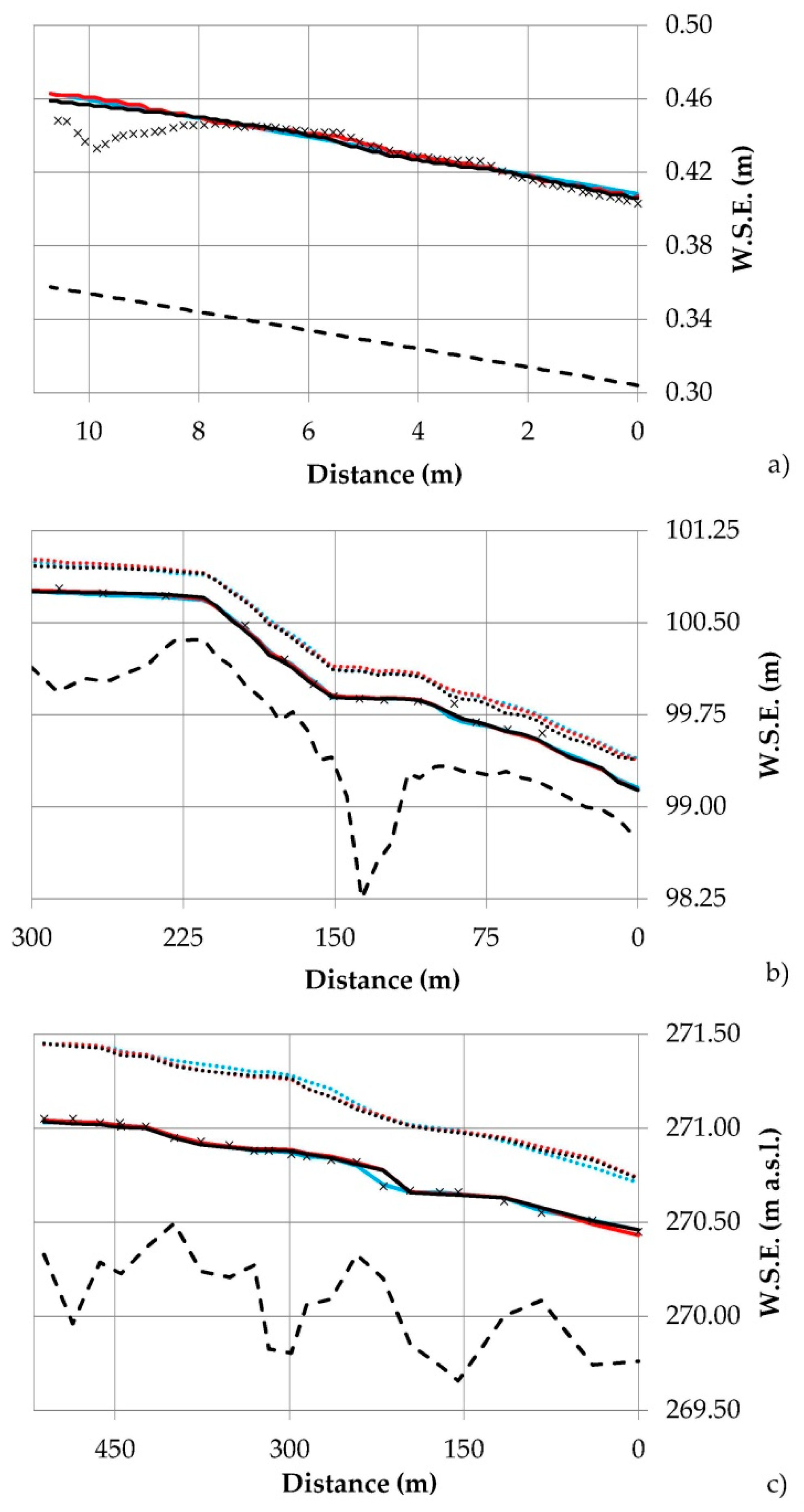
In the course of the calibration, the flow resistances were adjusted in the numerical models until a match with measured water surface elevations was achieved. Good agreements with average differences below 1 cm between measurements and simulations were obtained for C.1 (Figure 2a—solid lines) for all numerical models excluding the inlet area between distance 10.5 m and 9.5 m, where maximum differences of 3 cm occurred, which are related to issues of the physical model setup. The calibrated roughness values are = 52 m1/3 s−1 for the 1D and 2D model and = 0.005 m for the 3D model.
In C.2 (Figure 2b—solid lines), comparisons of measurements and numerical calculations show average differences of 2 cm excluding maximum outliers of 12 cm (1D) and 9 cm (2D and 3D) at a distance of 90 m. The single occurrence of the outlier indicates a local measurement issue. Best agreement was achieved by employing roughness values in section 215–150 m of = 9.1/9.0 m1/3 s−1 (1D/2D-model) and = 1.5 m (3D model), while the areas up- and downstream of this section (300–215 m and 150–0 m) received roughness values of = 18.2/18.0 m1/3 s−1 (1D/2D) and = 0.25 m (3D model). The higher flow resistance in section 215–150 m reflects the stronger turbulent flow conditions in this area, which is characterized by a steeper bed slope and coarser bed sediments.
The average differences in C.3 (Figure 2c) are below 1 cm except the comparison at distance 220 m, where outliers of 9 cm (2D) and 8 cm (3D) occur. The single occurrence of the outlier again indicates a local measurement issue. The calibrated roughness values in C.3 are = 25.0 m1/3 s−1 for the 1D and 2D model and = 0.20 m for the 3D model.
In the natural river sites (C.2 and C.3), additional discharge scenarios, defined by the mean discharge of each area (Table 3), have been simulated with the same roughness values and are depicted in Figure 2b,c with dotted lines. Due to lack of data, an evaluation with measurements was not possible, but the results were compared among each other. In C.2 (Figure 2b—dotted lines) the maximum average difference of 3 cm occurred between 2D and 3D simulations, while the maximum average difference in C.3 (Figure 2c—dotted lines) was 1 cm, determined between 1D and 3D simulations.
3.2. Sensitivity Analysis of Roughness Values in the Case of High Flow Conditions
The difficulties of using numerical simulations in cases of high flow conditions () without monitoring data is assessed in the form of a sensitivity analysis in C.2, demonstrating the differences between various models and the influences of changing roughness values. The water surface elevations simulated by 1D (blue solid line), 2D (red solid line) and 3D (black solid line) models is shown in Figure 3 including a bandwidth (dotted lines with corresponding colors) calculated with roughness values, which were changed by +/−20% referred to calibration (Section 3.1). Good agreements were found between 1D and 2D simulations, using roughness values of calibration resulting in average difference of around 5 cm, while the comparison to 3D simulations yields increasing differences starting with values of 1 cm at the outflow boundary (river section 0 m) up to 60 cm at the inflow boundary (river section 300 m). Following a roughness reduction of 20% in the case of 1D and 2D models, the highest differences compared to 3D simulations at reference conditions reduce to 40 cm, while a roughness increase of 20% in the case of 3D modelling leads to the smallest differences of 15 cm compared to 1D using roughness values of the calibration.
3.3. Analysis of Bed Shear Stresses
Bed shear stresses simulated in C.1 are depicted in Figure 4a for all numerical models. In the case of the 1D simulation, the bed shear stresses are 4.9 Nm−2 without any differences in the lateral or longitudinal direction. Along the thalweg, similar values are obtained in the higher dimensional models, but due to the two consecutive bends higher bed shear stresses up to 6.5 Nm−2 and 10.0 Nm−2 occur along the inner banks of the 2D and 3D simulations, respectively, while the outer banks are characterized by lower values of around 2.0/0.4 Nm−2 (2D/3D).
In C.2 at mean flow conditions (; Figure 4b), the highest bed shear stresses arise in the area between cross-sections 21 and 30, which is a riffle section [72] with low water depths, high flow velocities as well as high roughness values, resulting in values of 79/108/93 Nm−2 depending on the model dimension (1D/2D/3D). In the other sections, the bed shear stresses are substantially lower with values between 2 and 16 Nm−2 upstream the riffle section and between 2 and 41 Nm−2 downstream of this section in all models. Independent of the section, it is obvious that the 1D model is not able to predict any lateral variability, leading to higher values at the river banks and lower bed shear stresses in the main stream compared to higher dimensional models. In addition, it is shown that the values in the main stream of the 2D model tend to be larger in comparison to the 3D model, while at the banks a slight reverse trend occurs.
The modelling results of C.3 at mean flow conditions (; Figure 4c) also yield the highest bed shear stresses in the riffle sections, which are located between cross-sections 7 and 11 (21/33/44 Nm−2 for 1D/2D/3D) as well as cross-section 16 and 19 (13/16/19 Nm−2 for 1D/2D/3D), and are independent of the model dimension. While in the 2D simulations, the peaks occur in the main stream of the river, the highest values in the 3D simulation arise at the river banks. The reduced spatial discretization in the case of 1D simulations is again shown by constant values in the lateral direction.
3.4. Generalized Comparison of Numerical Models
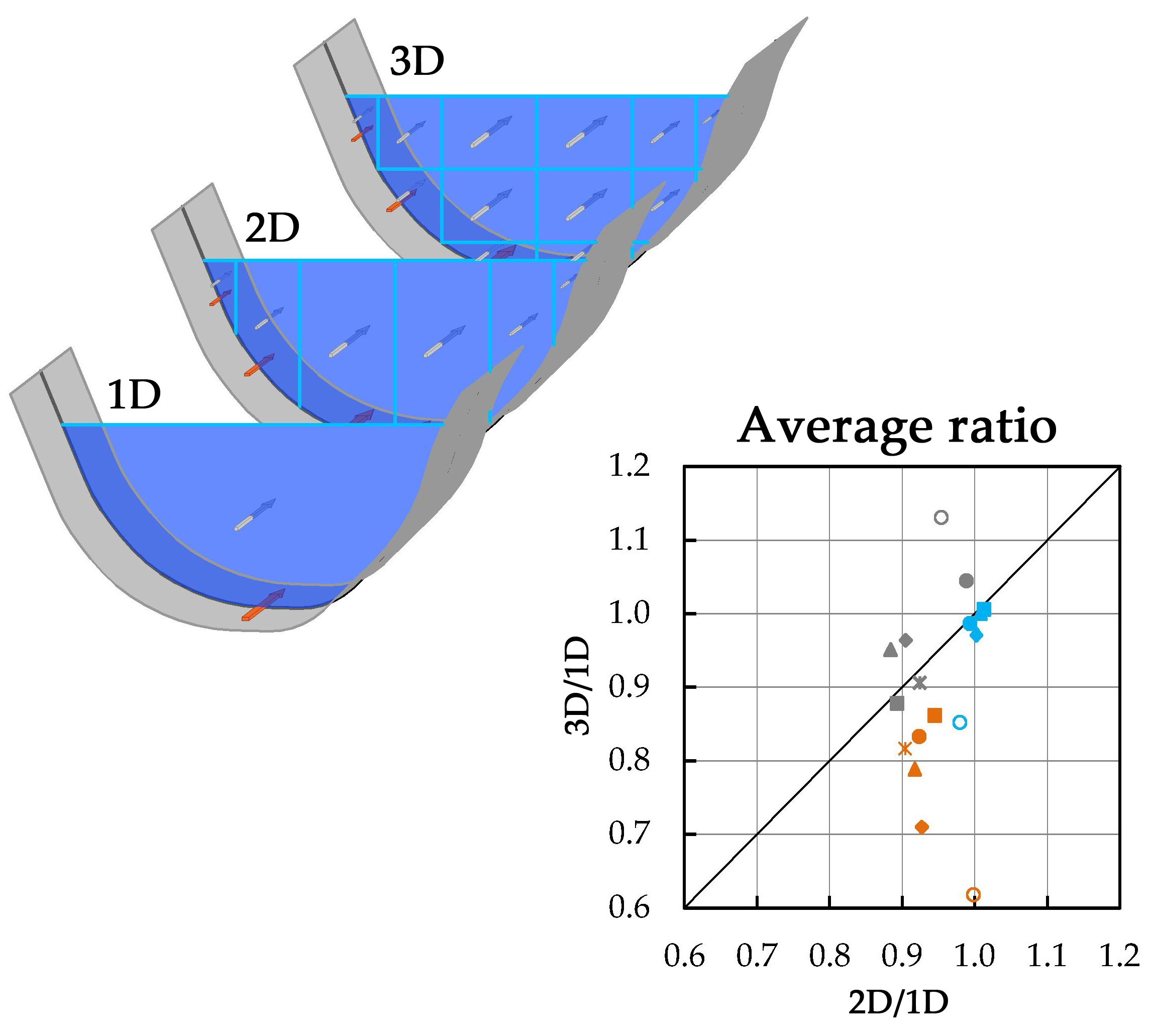
A generalized representation of modelling results including water depths, depth-averaged flow velocities and bed shear stresses is depicted in Figure 5 for all case studies and discharge scenarios. The water depth ratio between 2D/1D and 3D/1D (Figure 5a) at low flow and mean flow conditions is almost unity, stating that no substantial differences in the calculated water depths occurred by numerical models of different dimensions. An exception is the ratio 3D/1D at high flow conditions with quartiles of 0.80 and 0.90. Figure 5b shows the depth-averaged flow velocity ratio between 2D/1D and 3D/1D for all scenarios. The quartiles in the case of 2D/1D are between 0.64 and 1.23 and 0.61 and 1.43 in the case of 3D/1D. The bed shear stress ratios between 2D/1D and 3D/1D (Figure 5c) are characterized by quartiles of 0.45 and 1.28 and 0.43 and 1.15, respectively. Additionally, a summarized analysis (Figure 5d) including the averaged ratio between 2D and 3D values referred to 1D values shows almost no differences in the case of water depths (blue) at low flow and mean flow conditions resulting in values close to unity. An exception is the ratio 3D/1D at high flow conditions with a value of 0.85. In the case of flow velocities (grey), averaged ratios of 0.88 to 0.99 (2D/1D) and 0.88 to 1.13 (3D/1D) were obtained, whereby the ratios increase with the discharges in each case study. The largest deviations were found again for bed shear stresses (brown) with values of 0.90 to 1.00 (2D/1D) and 0.62 to 0.86 (3D/1D). Independent of the scenario, the calculated ratios are below the line of perfect agreement, indicating on average lower bed shear stresses in 3D models compared to 2D models.
Although models were calibrated to water surface elevations, the results exhibit clear differences in bed shear stress ratios. While in the case of 2D/1D, minor differences are noticed between the different river sites and discharges, the ratio decreased in the case of 3D/1D from lower to higher discharges (→ and →) as well as from small-sloped to steeper river sites (C.3→C.2).
3.5. Detailed Anaylsis of Simulated Hydrodynamics in Cross-Sections
Figure 6 depicts the simulated hydrodynamics of all model dimensions including bed shear stresses, flow velocities, turbulent kinetic energy (3D) and water surface elevations in three representative cross-sections of all case studies (CS 49 of C.1, CS 28 of C.2, CS 17 of C.3—encircled in Figure 1). The different model dimensions are based on various definitions of flow velocities. The area-averaged flow velocity (light grey solid line) in the case of 1D, the depth-averaged flow velocity (2D—dark grey solid line) and the near-wall tangential flow velocity (3D—black solid line), which equals the near-wall flow velocity in the case of small bed cell slopes.
The area-averaged flow velocity in CS 49 of C.1 (Figure 6a) is constant with a value of 0.79 m s−1. The profile of the 2D depth-averaged flow velocities is characterized by a maximum of 0.84 m s−1 close to the left bank and a minimum of 0.41 m s−1 on the right bank. A similar profile was calculated for the near-wall tangential flow velocity in the 3D model, whereby the values are substantially lower, characterized by a peak of 0.72 m s−1 and a minimum of 0.10 m s−1. The near-wall turbulent kinetic energy follows a falling trend starting with the highest value (0.04 m2 s−2) at the left bank and ending with the lowest value at the right bank (0.01 m2 s−2). The water depths are almost equal in all models with an average value of 0.43 m, whereby slight increasing trends from the left to the right bank occur in the 2D and 3D models. Due to the trapezoidal channel geometry, the lowest water depths arise at the banks. The comparison of bed shear stresses displays the dependency of this variable on flow velocities, turbulent kinetic energies and water depths. In the case of 2D, the profile of the bed shear stresses is similar to the profile of the flow velocities resulting in a maximum of 5.8 Nm−2 in the area of the left bank and a minimum of 2.0 Nm−2 close to the right bank, but due to the influence of the water depths an offset between the peaks of bed shear stress and flow velocity occurs. Comparable results were found in the case of 3D models, where similarities occur between the profiles of the near-wall tangential flow velocities and bed shear stresses, with a maximum (10.2 Nm−2) on the left bank and a minimum (0.4 Nm−2) on the right bank. However, the strong influence of the turbulent kinetic energy is obvious particularly at the left bank resulting in the highest bed shear stresses of the entire cross-section. In contrast, the one-dimensional approach results in a constant value of 4.8 Nm−2 in the whole cross-section.
In CS 28 of C.2 (Figure 6b), the area-averaged flow velocity is constant with a value of 0.54 m s−1. In the case of 2D, the profile of the depth-averaged flow velocities is characterized by a maximum of 0.69 m s−1 in the main stream of the river located at distance 11 m of the cross-section. Similarities are present for the profile of the near-wall tangential flow velocity in the 3D model with a peak of 0.64 m s−1. The near-wall turbulent kinetic energies are characterized by a relative constant plateau in the cross-section center (11–19 m) with values between 0.70 and 0.80 m2 s−1, a decreasing tendency to the banks and peaks up to 0.83 m2 s−1 on the banks. The water surface elevations are almost equal in all models with an average value of 100.68 m. Due to the straight river course in this cross-section, the water surface elevations do not change between the banks, hence the water depths only depend on the channel geometry. The comparison of bed shear stresses again indicates the dependency of this variable of flow velocities, turbulent kinetic energies and water depths. In the case of 2D as well as 3D, the profile of the bed shear stresses is similar to the profile of the depth-averaged and tangential flow velocities, resulting in maxima of 65.9 and 63.3 Nm−2 in the main stream of the river. However, the influence of the turbulent kinetic energy is visible at the right bank, resulting in a peak of 11.0 Nm−2. In contrast, the one-dimensional approach leads to a constant value of 44.0 Nm−2 in the whole cross-section.
The hydrodynamic variables for low flow (Figure 6c) and mean flow conditions (Figure 6d) are depicted for CS 17 of C.3. The area-averaged flow velocity is constant over the whole cross-section with values of 0.65 m s−1 () and 0.66 m s−1 (). The profile of the 2D depth-averaged flow velocities is characterized by a maximum of 0.68 m s−1 () and 0.96 m s−1 (), located in the main stream of the river. A similar profile was calculated for the near-wall tangential flow velocity in the 3D model, whereby the values are substantially lower with a peak of 0.41 m s−1 () and 0.59 m s−1 ().
The near-wall turbulent kinetic energies are characterized by values of 0.03–0.04 m2 s−2 (), and 0.03–0.045 m2 s−2 () in the main stream and peaks up to 0.14 m2 s−2 (), and 0.10 m2 s−2 () at the banks. The water surface elevations are almost equal in all models with an average value of 270.95 m a.s.l. at low flow conditions and 271.36/271.34/271.33 m a.s.l. (1D/2D/3D) at mean flow conditions. Due to the straight river course in this cross-section, the water surface elevations do not vary between the banks, thus the water depths only depend on the present geometry. The comparison of bed shear stresses again displays the dependency of this variable on flow velocities, turbulent kinetic energies and water depths. Independent of the discharge, the profiles of the bed shear stresses calculated in the 2D model follow the profiles of the depth-averaged flow velocities, resulting in peak values of 9.4 Nm−2 () and 15.7 Nm−2 () in the main stream of the river. In the 3D model, comparable results were found in the main stream, where similarities between the profiles of the near-wall tangential flow velocities and bed shear stresses occur, with a maximum of 8.4 Nm−2 () and 12.2 Nm−2 (). However, the strong influence of the turbulent kinetic energies close to the banks is obvious leading to the highest bed shear stresses of 9.4/15.8 Nm−2 (/) in the entire cross-section. In contrast, the one-dimensional approach results in a constant value of 9.9/8.6 Nm−2 (/) in the whole cross-section.
4. Discussion
The comparison of simulation results calculated in different model dimensions in general involves the risk of potential result dependencies on the applied spatial discretization. In order to overcome these issues, a sensitivity analysis including a variation of horizontal node distances was performed to ensure grid-independent solutions. However, in the case of 3D simulations the vertical discretization must be considered as well. In engineering practice, this discretization is usually a justified compromise between computational time and numerical accuracy. Hence, in sediment transport simulations, for which a correct prediction of the shear stress parameter is paramount, which depends on the vertical discretization, literature reports the usage of typically five to eight layers; good agreement with measurements has shown to justify this choice [53,58,59,69]. In line with this practice, the simulations in this study were performed with six layers.
Based on grid independency, the numerical models were successfully calibrated at low flow conditions. Although all site-specific heterogeneities (e.g., bed sediments, channel units and vegetation) have to be aggregated in roughness values, good agreement with measured water surface elevations was achieved in all areas investigated. The study shows that the roughness values are constant along the river course in all case studies except C.2, where a substantial coarsening of sediments in a riffle section led to a lower Strickler value and a higher equivalent sand roughness, respectively. The determined values are in line with guidelines [41,42,43].
However, the comparison of simulation results calculated by different model dimensions shows that the largest differences were found for bed shear stresses, due to the following reasons: (i) The averaged comparison ratio is lower than unity because of the area-averaged approach in the case of 1D models resulting in overestimations in bank areas. (ii) Moreover, the values are lower in general in the case of 3D compared to 2D simulations, which has also been reported by Lane et al. [80] and is based on the different calculation approaches. The bed shear stress calculations in 2D models are based on the depth-averaged flow velocities, which are in general higher than the near-wall flow velocities used in 3D models. (iii) Additionally, it was shown that the averaged comparison ratio between 3D/2D and 3D/1D is decreasing with increasing discharges, independent of the case study. This fact is again related to the different calculation approaches based on the corresponding roughness definitions.
A closer look into the different roughness definitions reveals the known fact that the Strickler value is a variable depending on the water depth and thus actually has to be adjusted according to the discharge (Ferguson [1]), while the equivalent sand roughness can be considered as constant as long as the river bed is stable. Jäggi [40] suggested an improved calculation of the Strickler value depending on the water depth, which leads to increasing values—exemplarily calculated for case study C.2 to be 16/19/27 m1/3 s−1 (//)—while in this study, in line with predominant hydraulic engineering practice, the roughness is kept constant at 18 m1/3 s−1. In particular, the large differences in the case of high flow conditions have to be highlighted, which result in substantially higher bed shear stresses as well as water surface elevations calculated by the 1D and 2D models compared to the 3D model.
According to Jäggi [40], Lamb et al. [81] and Parker et al. [82], the Strickler value is additionally increasing with decreasing bed slopes. Considering this and the calculation of bed shear stresses in 1D and 2D models, where high values result in low bed shear stresses, the decreasing 3D/1D ratios from small-sloped to steeper river sites (C.3→C.2) become obvious. Due to the fact that several parameters (e.g., water depth, equivalent sand roughness, etc.) vary between the different case studies, only this overall tendency can be identified.
A comparison to measure bed shear stresses could be a remedy to overcome the issue of considerable differences between the models. However, monitoring this parameter itself [83] is an ongoing challenge. Besides issues of handling the devices (installation, operation and service), concerns about the validity and explanatory power of time-averaged bed shear stresses were raised. Gmeiner et al. [84] and Liedermann et al. [85] showed that bed load transport takes place below expected discharges considering the concepts of Shields [86] and Zanke [87] for critical shear stresses. It is thus recommended to consider time series of bed shear stresses including fluctuations for which probabilistic approaches [88,89,90,91] are suitable. A part of these fluctuations is expected to be covered by considering the turbulent kinetic energies for calculating bed shear stresses in the case of 3D models. In this study, the dependency of bed shear stresses on turbulent kinetic energies are highlighted by peaks at the banks, which correlate with peaks of the turbulent kinetic energy. A proportional relationship between turbulent kinetic energy and bed shear stress for high strains has already been described by Menter [92]. Additionally, Rodi [93] stated an increasing influence of turbulence on shear stresses upon larger roughness values.
The aforementioned uncertainties of using deterministic bed shear stress calculations, as well as the additional limitations when employing these concepts in numerical models should always be considered by addressing the issues related to dependent processes including bed load transport or morphological changes. Particularly in the case of man-made interventions [94], including engineering measures [95] in rivers, reservoirs or oceans as well as management procedures [96] such as flushing, dredging or depositing sediments, it is recommended to focus on the evaluation of differences rather than on absolute values. In general, improving the results of 1D and 2D models by applying discharge-dependent Strickler values and preferring higher dimensional models over lower ones has the potential to enhance the validity of numerical simulations.
5. Conclusions
The application of numerical models in hydraulic engineering has become routine over recent decades, resulting in numerous published studies. Standard practice is the calibration of a single numerical model by comparing simulation results to monitoring data (e.g., water surface elevations, flow velocities, etc.) followed by an application of the models for any kind of work. Despite known uncertainties (e.g., model simplifications, mesh generation, roughness definition, etc.), it is generally assumed that the simulated results are valid for all hydrodynamic parameters, including properties for which no measurements are available. The present study addressed the differences between model dimensions, focusing on bed shear stresses considering different discharges as well as study sites.
The results show that, on average, the simulated bed shear stresses are 10% and 14–38% lower in the applied 2D and 3D model, respectively, as compared to the 1D model. At the same time, almost no differences were present in water surface elevations, which had been used for calibration. When comparing different river sites and discharges, minor differences in the ratio of bed shear stresses were found in 2D/1D models, while in the case of 3D/1D the differences became larger from lower to higher discharges as well as from small-sloped to steeper river sites. The major influence of different roughness definitions, as well as the various calculation approaches used in the numerical models, were identified as a cause of these differences. Moreover, reasons why, in general, the highest bed shear stresses in the main stream of the river occur in 2D models (e.g., depth-averaged versus near-bed flow velocities), and for bed shear stress peaks at the banks in 3D models were elaborated (e.g., consideration of turbulent kinetic energy).
The considerable differences between the numerical models present an issue in hydraulic engineering, due to the fact that bed shear stresses form the basis of many approaches including the calculation of sediment transport or evaluation of habitats. One of the key tasks of future works will be the comparison with measurement data considering the associated monitoring challenges. The question of whether the deterministic approach of calculating bed shear stresses, as well as the definition of bed shear stress, is adequately representing the occurring near-bed forces in an applied river context should also be addressed in future studies.
Author Contributions
K.G., M.T. and C.H. designed, set up and performed the numerical simulations and analyzed the results including the comparison with measurements as well as between the models. The draft text was prepared by K.G. and edited by M.T., C.H. and H.H.
Funding
This paper was written as a contribution to the Christian Doppler Laboratory for Sediment Research and Management. The financial support by the Austrian Federal Ministry for Digital and Economic Affairs and the National Foundation for Research, Technology and Development is gratefully acknowledged.
Acknowledgments
The authors thank the Hydraulic Engineering Institute of the University of Innsbruck for providing measurement data of the laboratory experiment.
Conflicts of Interest
The authors declare no conflict of interest.
References
- Ferguson, R. Time to abandon the Manning equation? Earth Surf. Process. Landf. 2010, 35, 1873–1876. [Google Scholar] [CrossRef]
- Powell, D.M. Flow resistance in gravel-bed rivers: Progress in research. Earth-Sci. Rev. 2014, 136, 301–338. [Google Scholar] [CrossRef]
- Järvelä, J. Flow Resistance in Environmental Channels: Focus on Vegetation; Helsinki University of Technology Water Resources Publications: Helsinki, Finland, 2004. [Google Scholar]
- Green, J.C. Modelling flow resistance in vegetated streams: Review and development of new theory. Hydrol. Process. 2004, 19, 1245–1259. [Google Scholar] [CrossRef]
- Manga, M.; Kirchner, J.W. Stress partitioning in streams by large woody debris. Water Resour. Res. 2000, 36, 2373–2379. [Google Scholar] [CrossRef] [Green Version]
- Wilcox, A.C.; Wohl, E.E. Flow resistance dynamics in step-pool stream channels: 1. Large woody debris and controls on total resistance. Water Resour. Res. 2006, 42. [Google Scholar] [CrossRef]
- Wilcox, A.C.; Nelson, J.M.; Wohl, E.E. Flow resistance dynamics in step-pool channels: 2. Partitioning between grain, spill, and woody debris resistance. Water Resour. Res. 2006, 42. [Google Scholar] [CrossRef] [Green Version]
- Parker, G.; Peterson, A.W. Bar resistance of gravel-bed streams. J. Hydraul. Div. 1980, 106, 1559–1575. [Google Scholar]
- Prestegaard, K.L. Bar resistance in gravel bed streams at bankfull stage. Water Resour. Res. 1983, 19, 472–476. [Google Scholar] [CrossRef]
- Hey, R.D. Bar Form Resistance in Gravel-Bed Rivers. J. Hydraul. Eng. 1988, 114, 1498–1508. [Google Scholar] [CrossRef]
- Millar, R.G. Grain and form resistance in gravel-bed rivers Résistances de grain et de forme dans les rivières à graviers. J. Hydraul. Res. 1999, 37, 303–312. [Google Scholar] [CrossRef]
- Francalanci, S.; Solari, L.; Toffolon, M.; Parker, G. Do alternate bars affect sediment transport and flow resistance in gravel-bed rivers? Earth Surf. Process. Landf. 2012, 37, 866–875. [Google Scholar] [CrossRef] [Green Version]
- Wohl, E.E.; Thompson, D.M. Velocity characteristics along a small step–pool channel. Earth Surf. Process. Landf. 2000, 25, 353–367. [Google Scholar] [CrossRef]
- Curran, J.H.; Wohl, E.E. Large woody debris and flow resistance in step-pool channels, Cascade Range, Washington. Geomorphology 2003, 51, 141–157. [Google Scholar] [CrossRef]
- Church, M.; Zimmermann, A. Form and stability of step-pool channels: Research progress. Water Resour. Res. 2007, 43. [Google Scholar] [CrossRef]
- Wilcox, A.C.; Wohl, E.E. Field measurements of three-dimensional hydraulics in a step-pool channel. Geomorphology 2007, 83, 215–231. [Google Scholar] [CrossRef]
- Comiti, F.; Mao, L. Recent Advances in the Dynamics of Steep Channels. Gravel Bed Rivers 2012. [Google Scholar] [CrossRef]
- Comiti, F.; Cadol, D.; Wohl, E. Flow regimes, bed morphology, and flow resistance in self-formed step-pool channels. Water Resour. Res. 2009, 45. [Google Scholar] [CrossRef]
- Song, T.; Chiew, Y.M.; Chin, C.O. Effect of Bed-Load Movement on Flow Friction Factor. J. Hydraul. Eng. 1998, 124, 165–175. [Google Scholar] [CrossRef]
- Bergeron, N.E.; Carbonneau, P. The effect of sediment concentration on bedload roughness. Hydrol. Process. 1999, 13, 2583–2589. [Google Scholar] [CrossRef]
- Calomino, F.; Gaudio, R.; Miglio, A. Effect of bed-load concentration on friction factor in narrow channels. In Proceedings of the 2nd International Conference on Fluvial Hydraulics–River Flow, Naples, Italy, 23–25 June 2004; Taylor and Francis Group: London, UK, 2004; pp. 279–285. [Google Scholar]
- Gao, P.; Abrahams, A.D. Bedload transport resistance in rough open-channel flows. Earth Surf. Process. Landf. 2004, 29, 423–435. [Google Scholar] [CrossRef]
- Campbell, L.; McEwan, I.; Nikora, V.; Pokrajac, D.; Gallagher, M.; Manes, C. Bed-Load Effects on Hydrodynamics of Rough-Bed Open-Channel Flows. J. Hydraul. Eng. 2005, 131, 576–585. [Google Scholar] [CrossRef] [Green Version]
- Recking, A.; Frey, P.; Paquier, A.; Belleudy, P.; Champagne, J.Y. Feedback between bed load transport and flow resistance in gravel and cobble bed rivers. Water Resour. Res. 2008, 44. [Google Scholar] [CrossRef] [Green Version]
- Recking, A.; Frey, P.; Paquier, A.; Belleudy, P.; Champagne, J.Y. Bed-Load Transport Flume Experiments on Steep Slopes. J. Hydraul. Eng. 2008, 134, 1302–1310. [Google Scholar] [CrossRef]
- Fischenich, C. Robert Manning (A Historical Perspective); EMRRP Technical Notes Collection (ERDCTN-EMRRP-SR-10), U.S. Army Engineer Research and Development Center: Vicksburg, MS, USA, 2000. [Google Scholar]
- Brown, G.O. The History of the Darcy-Weisbach Equation for Pipe Flow Resistance. In Environmental and Water Resources History; ASCE Civil Engineering Conference and Exposition: Washington, DC, USA, 2002; pp. 34–43. [Google Scholar]
- Simmons, C.T. Henry Darcy (1803–1858): Immortalised by his scientific legacy. Hydrogeol. J. 2008, 16, 1023–1038. [Google Scholar] [CrossRef]
- Zimmermann, A. Flow resistance in steep streams: An experimental study. Water Resour. Res. 2010, 46. [Google Scholar] [CrossRef]
- Bathurst, J.C. Flow resistance of large-scale roughness. J. Hydraul. Div. 1978, 104, 1587–1603. [Google Scholar]
- Bathurst, J.C. At-a-site variation and minimum flow resistance for mountain rivers. J. Hydrol. 2002, 269, 11–26. [Google Scholar] [CrossRef]
- Katul, G.; Wiberg, P.; Albertson, J.; Hornberger, G. A mixing layer theory for flow resistance in shallow streams. Water Resour. Res. 2002, 38, 32-1–32-8. [Google Scholar] [CrossRef]
- Lee, A.J.; Ferguson, R.I. Velocity and flow resistance in step-pool streams. Geomorphology 2002, 46, 59–71. [Google Scholar] [CrossRef]
- Smart, G.M.; Duncan, M.J.; Walsh, J.M. Relatively Rough Flow Resistance Equations. J. Hydraul. Eng. 2002, 128, 568–578. [Google Scholar] [CrossRef]
- Aberle, J.; Smart, G.M. The influence of roughness structure on flow resistance on steep slopes. J. Hydraul. Res. 2003, 41, 259–269. [Google Scholar] [CrossRef]
- Canovaro, F.; Solari, L. Dissipative analogies between a schematic macro-roughness arrangement and step–pool morphology. Earth Surf. Process. Landf. 2007, 32, 1628–1640. [Google Scholar] [CrossRef] [Green Version]
- Ferguson, R. Flow resistance equations for gravel- and boulder-bed streams. Water Resour. Res. 2007, 43. [Google Scholar] [CrossRef] [Green Version]
- Strickler, A. Beiträge zur Frage der Geschwindigkeitsformel und der Rauhigkeitszahlen für Ströme, Kanäle und geschlossene Leitungen; Eidgenossisches Amt für Wasserwirtschaft: Bern, Switzerland, 1923. [Google Scholar]
- Meyer-Peter, E.; Müller, R. Formulas for bed-load transport. In Proceedings of the 2nd Meeting of IAHR, Stockholm, Sweden, 7–9 June 1948; IAHR: Stockholm, Sweden, 1948; pp. 39–64. [Google Scholar]
- Jäggi, M. Alternierende Kiesbänke: Untersuchungen über ihr Auftreten, den Zusammenhang mit der Bildung von Sohlenformen im allgemeinen, sowie ihre Auswirkungen auf Ufererosion und Fliesswiderstand; Versuchsanstalt für Wasserbau, Hydrologie, und Glaziologie: ETH Zurich, Switzerland, 1983. [Google Scholar]
- Chow, V.T. Open Channel Hydraulics; McGraw-Hill: New York, NY, USA, 1959. [Google Scholar]
- Naudascher, E. Hydraulik der Gerinne und Gerinnebauwerke, 2nd ed.; Springer: Vienna, Austria, 1992. [Google Scholar]
- US Army Corps of Engineers. Engineering and Design—Hydraulic Design of Flood Control Channels; American Society of Civil Engineers: New York, NY, USA, 1994; Volume 10. [Google Scholar]
- Horton, R.E. Separate Roughness Coefficients for Channel Bottom and Sides. Eng. News-Rec. 1933, 3, 652–653. [Google Scholar]
- Einstein, H.A. Der hydraulische oder Profil-Radius. Schweiz. Bauztg. 1934, 103, 89–91. [Google Scholar]
- Krishnamurthy, M.; Christensen, B.A. Equivalent roughness for shallow channel. J. Hydraul. Div. 1972, 98, 2257–2263. [Google Scholar]
- Yen Ben, C. Open Channel Flow Resistance. J. Hydraul. Eng. 2002, 128, 20–39. [Google Scholar] [CrossRef] [Green Version]
- Järvelä, J. Effect of submerged flexible vegetation on flow structure and resistance. J. Hydrol. 2005, 307, 233–241. [Google Scholar] [CrossRef]
- Nepf, H.M. Hydrodynamics of vegetated channels. J. Hydraul. Res. 2012, 50, 262–279. [Google Scholar] [CrossRef] [Green Version]
- Aberle, J.; Järvelä, J. Flow resistance of emergent rigid and flexible floodplain vegetation. J. Hydraul. Res. 2013, 51, 33–45. [Google Scholar] [CrossRef]
- Nikuradse, J. Strömungsgesetze in Rauhen Rohren; VDI-Verlag: Berlin, Germany, 1933; Volume 361. [Google Scholar]
- Booker, D.J.; Sear, D.A.; Payne, A.J. Modelling three-dimensional flow structures and patterns of boundary shear stress in a natural pool–riffle sequence. Earth Surf. Process. Landf. 2001, 26, 553–576. [Google Scholar] [CrossRef]
- Fischer-Antze, T.; Olsen, N.R.B.; Gutknecht, D. Three-dimensional CFD modeling of morphological bed changes in the Danube River. Water Resour. Res. 2008, 44. [Google Scholar] [CrossRef]
- Rüther, N.; Jacobsen, J.; Olsen, N.R.B.; Vatne, G. Prediction of the three-dimensional flow field and bed shear stresses in a regulated river in mid-Norway. Hydrol. Res. 2010, 41, 145–152. [Google Scholar] [CrossRef]
- Guerrero, M.; Lamberti, A. Bed-roughness investigation for a 2-D model calibration: The San Martín case study at Lower Paranà. Int. J. Sediment Res. 2013, 28, 458–469. [Google Scholar] [CrossRef]
- Guerrero, M.; Latosinski, F.; Nones, M.; Szupiany, R.N.; Re, M.; Gaeta, M.G. A sediment fluxes investigation for the 2-D modelling of large river morphodynamics. Adv. Water Resour. 2015, 81, 186–198. [Google Scholar] [CrossRef]
- Paarlberg, J.A.; Guerrero, M.; Huthoff, F.; Re, M. Optimizing Dredge-and-Dump Activities for River Navigability Using a Hydro-Morphodynamic Model. Water 2015, 7, 3943–3962. [Google Scholar] [CrossRef] [Green Version]
- Glas, M.; Glock, K.; Tritthart, M.; Liedermann, M.; Habersack, H. Hydrodynamic and morphodynamic sensitivity of a river’s main channel to groyne geometry. J. Hydraul. Res. 2018, 56, 714–726. [Google Scholar] [CrossRef]
- Glock, K.; Tritthart, M.; Gmeiner, P.; Pessenlehner, S.; Habersack, H. Evaluation of engineering measures on the Danube based on numerical analysis. J. Appl. Water Eng. Res. 2017, 1–19. [Google Scholar] [CrossRef]
- Nicholas, A.P.; Sandbach, S.D.; Ashworth, P.J.; Amsler, M.L.; Best, J.L.; Hardy, R.J.; Lane, S.N.; Orfeo, O.; Parsons, D.R.; Reesink, A.J.H.; et al. Modelling hydrodynamics in the Rio Paraná, Argentina: An evaluation and inter-comparison of reduced-complexity and physics based models applied to a large sand-bed river. Geomorphology 2012, 169–170, 192–211. [Google Scholar] [CrossRef]
- Xie, Q.; Yang, J.; Lundström, S.; Dai, W. Understanding Morphodynamic Changes of a Tidal River Confluence through Field Measurements and Numerical Modeling. Water 2018, 10, 1424. [Google Scholar] [CrossRef]
- Einstein, H.A. The Bed-Load Function for Sediment Transportation in Open Channel Flows; US Department of Agriculture: Washington, DC, USA, 1950; Volume 1026.
- Van Rijn Leo, C. Sediment Transport, Part I: Bed Load Transport. J. Hydraul. Eng. 1984, 110, 1431–1456. [Google Scholar] [CrossRef]
- Van Rijn, L.C. Principles of Sediment Transport in Rivers, Estuaries and Coastal Seas; Aqua Publications: Amsterdam, The Netherlands, 1993; Volume 1006. [Google Scholar]
- Wu, W.; Wang, S.S.Y.; Jia, Y. Nonuniform sediment transport in alluvial rivers. J. Hydraul. Res. 2000, 38, 427–434. [Google Scholar] [CrossRef]
- Bravo-Espinosa, M.; Osterkamp, W.R.; Lopes Vicente, L. Bedload Transport in Alluvial Channels. J. Hydraul. Eng. 2003, 129, 783–795. [Google Scholar] [CrossRef]
- Habersack, H.; Seitz, H.; Laronne, J.B. Spatio-temporal variability of bedload transport rate: Analysis and 2D modelling approach. Geodin. Acta 2008, 21, 67–79. [Google Scholar] [CrossRef]
- Riesterer, J.; Wenka, T.; Brudy-Zippelius, T.; Nestmann, F. Bed load transport modeling of a secondary flow influenced curved channel with 2D and 3D numerical models. J. Appl. Water Eng. Res. 2016, 4, 54–66. [Google Scholar] [CrossRef]
- Tritthart, M.; Schober, B.; Habersack, H. Non-uniformity and layering in sediment transport modelling 1: Flume simulations. J. Hydraul. Res. 2011, 49, 325–334. [Google Scholar] [CrossRef]
- Tritthart, M.; Liedermann, M.; Schober, B.; Habersack, H. Non-uniformity and layering in sediment transport modelling 2: River application. J. Hydraul. Res. 2011, 49, 335–344. [Google Scholar] [CrossRef]
- Wu, W. Depth-Averaged Two-Dimensional Numerical Modeling of Unsteady Flow and Nonuniform Sediment Transport in Open Channels. J. Hydraul. Eng. 2004, 130, 1013–1024. [Google Scholar] [CrossRef]
- Hauer, C.; Unfer, G.; Tritthart, M.; Formann, E.; Habersack, H. Variability of mesohabitat characteristics in riffle-pool reaches: Testing an integrative evaluation concept (FGC) for MEM-application. River Res. Appl. 2011, 27, 403–430. [Google Scholar] [CrossRef]
- Tritthart, M. Three-dimensional numerical modelling of turbulent river flow using polyhedral finite volumes. Wien. Mitt. Wasser-Abwasser-Gewässer 2005, 193, 1–179. [Google Scholar]
- Muhar, S.; Kainz, M.; Schwarz, M.; Jungwirth, M. Ausweisung Flusstypspezifisch Erhaltener Fliessgewässerabschnitte in Österreich: Fliessgewässer mit Einem Einzugsgebiet Grösser als 500 km² Ohne Bundesflüsse; Abt. I 3; Bundesministerium für Nachhaltigkeit und Tourismus (BMNT): Vienna, Austria, 1998. [Google Scholar]
- Versteeg, H.K.; Malalasekera, W. An Introduction to Computational Fluid Dynamics: The Finite Volume Method; Pearson Education: Harlow, UK, 2007. [Google Scholar]
- Schlichting, H.; Gersten, K. Grenzschicht-Theorie; Springer: Berlin, Germany, 2006. [Google Scholar]
- US Army Corps of Engineers. HEC-RAS River Analysis System, Hydraulic Reference Manual; US Army Corps of Engieers, Hydrologic Engineering Center: Davis, CA, USA, 2010. [Google Scholar]
- Nujic, M. Praktischer Einsatz Eines Hochgenauen Verfahrens für die Berechnung von Tiefengemittelten Strömungen; Mitteilungen des Institutes der Bundeswehr München: Munich, Germany, 1999. [Google Scholar]
- Pironneau, O. Finite Element Methods for Fluids; Wiley: New York, NY, USA, 1989. [Google Scholar]
- Lane, S.; Bradbrook, K.; Richards, K.; Biron, P.; Roy, A. The application of computational fluid dynamics to natural river channels: Three-dimensional versus two-dimensional approaches. Geomorphology 1999, 29, 1–20. [Google Scholar] [CrossRef]
- Lamb, M.P.; Dietrich, W.E.; Venditti, J.G. Is the critical Shields stress for incipient sediment motion dependent on channel-bed slope? J. Geophys. Res. Earth Surf. 2008, 113. [Google Scholar] [CrossRef]
- Parker, C.; Clifford, N.J.; Thorne, C.R. Understanding the influence of slope on the threshold of coarse grain motion: Revisiting critical stream power. Geomorphology 2011, 126, 51–65. [Google Scholar] [CrossRef] [Green Version]
- Gmeiner, P.; Liedermann, M.; Tritthart, M.; Habersack, H. Development and testing of a device for direct bed shear stress measurement. In Proceedings of the 2nd IAHR, Europe Conference, Munich, Germany, 27–29 June 2012. [Google Scholar]
- Gmeiner, P.; Liedermann, M.; Haimann, M.; Tritthart, M.; Habersack, H. Grundlegende Prozesse betreffend Hydraulik, Sedimenttransport und Flussmorphologie an der Donau. Österreichische Wasser Und Abfallwirtsch. 2016, 68, 208–216. [Google Scholar] [CrossRef] [Green Version]
- Liedermann, M.; Gmeiner, P.; Kreisler, A.; Tritthart, M.; Habersack, H. Insights into bedload transport processes of a large regulated gravel-bed river. Earth Surf. Process. Landf. 2017, 43, 514–523. [Google Scholar] [CrossRef]
- Shields, A. Application of Similarity Principles and Turbulence Research to Bed-Load Movement; United States Department of Agriculture, Soil Conservation Service: Pasadena, CA, USA, 1936.
- Zanke, U. Der Beginn der Geschiebebewegung als Wahrscheinlichkeitsproblem. Wasser Und Boden 1990, 1, 40–43. [Google Scholar]
- Einstein, H.A.; El-Samni, E.-S.A. Hydrodynamic Forces on a Rough Wall. Rev. Mod. Phys. 1949, 21, 520–524. [Google Scholar] [CrossRef] [Green Version]
- Grass, A.J. Initial instability of fine bed sand. J. Hydraul. Div. 1970, 96, 619–632. [Google Scholar]
- McEwan, I.; Heald, J. Discrete Particle Modeling of Entrainment from Flat Uniformly Sized Sediment Beds. J. Hydraul. Eng. 2001, 127, 588–597. [Google Scholar] [CrossRef]
- Ancey, C.; Heyman, J. A microstructural approach to bed load transport: Mean behaviour and fluctuations of particle transport rates. J. Fluid Mech. 2014, 744, 129–168. [Google Scholar] [CrossRef]
- Menter, F.R. Two-equation eddy-viscosity turbulence models for engineering applications. Aiaa J. 1994, 32, 1598–1605. [Google Scholar] [CrossRef] [Green Version]
- Rodi, W. Turbulence Modeling and Simulation in Hydraulics: A Historical Review. J. Hydraul. Eng. 2017, 143, 03117001. [Google Scholar] [CrossRef]
- Giardino, A.; Schrijvershof, R.; Nederhoff, C.M.; de Vroeg, H.; Brière, C.; Tonnon, P.K.; Caires, S.; Walstra, D.J.; Sosa, J.; van Verseveld, W.; et al. A quantitative assessment of human interventions and climate change on the West African sediment budget. Ocean Coast. Manag. 2018, 156, 249–265. [Google Scholar] [CrossRef]
- Habersack, H.; Piégay, H. 27 River restoration in the Alps and their surroundings: Past experience and future challenges. Dev. Earth Surf. Process. 2007, 11, 703–735. [Google Scholar]
- Hauer, C.; Wagner, B.; Aigner, J.; Holzapfel, P.; Flödl, P.; Liedermann, M.; Tritthart, M.; Sindelar, C.; Pulg, U.; Klösch, M.; et al. State of the art, shortcomings and future challenges for a sustainable sediment management in hydropower: A review. Renew. Sustain. Energy Rev. 2018, 98, 40–55. [Google Scholar] [CrossRef]
Figure 1.
Location of case studies in Austria (a); Overview of case studies including cross-sections used for a generalized comparison (grey and black lines) and the indicated cross-section for detailed analysis (encircled): Design of laboratory experiment representing C.1 (b), bed elevations of natural river site “Ybbs” representing C.2 (c) and bed elevations of natural river site “Sulm” representing C.3 (d).

Figure 2.
Calibration—Longitudinal profile plots of (a) C.1, (b) C.2 and (c) C.3 including bed elevations (dashed black line) and comparisons of measured (black crosses) and modelled water surface elevations (W.S.E.) at low flow () conditions (results of 1D simulations = blue solid line, 2D simulations = red solid line and 3D simulations = black solid line); Comparison of modelled W.S.E. at an additional discharge scenario (mean flow ) in C.2 and C.3 (results of 1D simulations = blue dotted line, 2D simulations = red dotted line and 3D simulations = black dotted line).

Figure 3.
Sensitivity analysis—Longitudinal profile plot of C.2 at high flow conditions () including bed elevations (dashed black line) and modelled water surface elevations (W.S.E.) (results of 1D simulations = blue solid line, 2D simulations = red solid line and 3D simulations = black solid line) with a bandwidth considering +/−20% of roughness changes (dotted lines with corresponding colors).

Figure 4.
Comparison of bed shear stresses calculated by 1D/2D/3D models depicted for (a) C.1, (b) C.2 at and (c) C.3 at .
Figure 4.
Comparison of bed shear stresses calculated by 1D/2D/3D models depicted for (a) C.1, (b) C.2 at and (c) C.3 at .

Figure 5.
Relative comparison of the modeling results of (a) water depths, (b) depth-averaged flow velocities and (c) bed shear stresses consisting of ratios between 3D and 2D values, referring to 1D values depicted in box-plots for each case study and discharge scenario; (d) Average ratio between 3D and 2D values, referring to 1D values for water depths (blue), flow velocities (grey) and bed shear stresses (brown) depicted for each case study and discharge scenario (C.1 (*), C.2- (▲), C.2- (♦), C.2- (○), C.3- (■), C.3- (●)).

Figure 6.
Detailed analysis of the hydrodynamics simulated by the 1D, 2D and 3D models in (a) CS 49 of C.1, (b) CS 28 of C.2 at , (c) CS 17 of C.3 at and (d) CS 17 of C.3 at including water surface elevations (blue dotted lines), bed shear stresses (brown large-spaced dashed lines), various flow velocities (area-averaged flow velocities (grey lines), depth-averaged flow velocities (dark grey lines), near wall tangential flow velocities (black lines)) and turbulent kinetic energies (green lines with rectangles) as well as bed elevations (black small-spaced dashed lines).


Table 1.
Overview of parameters, a and kS.
| Author | a | ks | Restriction |
|---|---|---|---|
| Strickler [38] | 21.1 | d90 | base layer |
| Meyer-Peter and Müller [39] | 26 | d90 | armor layer |
| USACE [43] | 29.4 | d50 | no limitation |
| Jäggi [40] | 2.0–23.3 | d90 | no limitation |
Table 2.
Overview of the spatial discretization of all the numerical models (h. = hexagonal, r. = rectangular, and t. = triangular mesh discretization).
Table 2.
Overview of the spatial discretization of all the numerical models (h. = hexagonal, r. = rectangular, and t. = triangular mesh discretization).
| Case Study | 1D | 2D | 3D | |||
|---|---|---|---|---|---|---|
| Cross-Sections | Discretization (m × m) | Computation Nodes | Discretization (m × m) | Vertical Layers | Computation Nodes | |
| C.1 | 109 | r. 0.1 × 0.03 | 7980 | r. 0.1 × 0.03 | 6 | 47,880 |
| C.2 | 43 | r. 1.0 × 1.0 | 18,918 | h. 1.0 × 1.0 | 6 | 59,220 |
| C.3 | 22 | t. 1.0 × 1.0 | 28,396 | h. 1.0 × 1.0 | 6 | 170,376 |
Table 3.
Overview of boundary conditions for all simulation scenarios.
| Acronym | Simulation Scenario | Inflow Boundary Discharge (m3/s) | Outflow Boundary | |
|---|---|---|---|---|
| Slope (-) | Water Level (m a.s.l.) | |||
| C.1 | Calibration | 0.09 | 0.005 | 0.394 |
| C.2—QL | Calibration | 1.64 | 0.005 | 99.140 |
| C.2—QM | Validation | 4.50 | 0.005 | 99.370 |
| C.2—HQ1 | High flow scenario | 64.00 | 0.005 | 101.073 |
| C.3—QL | Calibration | 2.66 | 0.0015 | 270.460 |
| C.3—QM | Validation | 8.85 | 0.0015 | 270.730 |
© 2019 by the authors. Licensee MDPI, Basel, Switzerland. This article is an open access article distributed under the terms and conditions of the Creative Commons Attribution (CC BY) license (http://creativecommons.org/licenses/by/4.0/).
Share and Cite
MDPI and ACS Style
Glock, K.; Tritthart, M.; Habersack, H.; Hauer, C. Comparison of Hydrodynamics Simulated by 1D, 2D and 3D Models Focusing on Bed Shear Stresses. Water 2019, 11, 226. https://doi.org/10.3390/w11020226
AMA Style
Glock K, Tritthart M, Habersack H, Hauer C. Comparison of Hydrodynamics Simulated by 1D, 2D and 3D Models Focusing on Bed Shear Stresses. Water. 2019; 11(2):226. https://doi.org/10.3390/w11020226
Chicago/Turabian StyleGlock, Kurt, Michael Tritthart, Helmut Habersack, and Christoph Hauer. 2019. "Comparison of Hydrodynamics Simulated by 1D, 2D and 3D Models Focusing on Bed Shear Stresses" Water 11, no. 2: 226. https://doi.org/10.3390/w11020226
Note that from the first issue of 2016, this journal uses article numbers instead of page numbers. See further details here.