Rainfall-Runoff Modelling Using Hydrological Connectivity Index and Artificial Neural Network Approach

Abstract

The input selection process for data-driven rainfall-runoff models is critical because input vectors determine the structure of the model and, hence, can influence model results. Here, hydro-geomorphic and biophysical time series inputs, including Normalized Difference Vegetation Index (NDVI) and Index of Connectivity (IC; a type of hydrological connectivity index), in addition to climatic and hydrologic inputs were assessed. Selected inputs were used to develop Artificial Neural Networks (ANNs) in the Haughton River catchment and the Calliope River catchment, Queensland, Australia. Results show that incorporating IC as a hydro-geomorphic parameter and remote sensing NDVI as a biophysical parameter, together with rainfall and runoff as hydro-climatic parameters, can improve ANN model performance compared to ANN models using only hydro-climatic parameters. Comparisons amongst different input patterns showed that IC inputs can contribute to further improvement in model performance, than NDVI inputs. Overall, ANN model simulations showed that using IC along with hydro-climatic inputs noticeably improved model performance in both catchments, especially in the Calliope catchment. This improvement is indicated by a slight increase (9.77% and 11.25%) in the Nash–Sutcliffe efficiency and noticeable decrease (24.43% and 37.89%) in the root mean squared error of monthly runoff from Haughton River and Calliope River, respectively. Here, we demonstrate the significant effect of hydro-geomorphic and biophysical time series inputs for estimating monthly runoff using ANN data-driven models, which are valuable for water resources planning and management.

1. Introduction

Runoff models are useful in water resources planning and management, drought management, design of hydraulic structures (e.g., dams, bridges, culverts), and flood forecasting. During the past several decades, hydrologists and engineers have typically applied rainfall-runoff (R-R) models using different combinations of hydrologic and climatic data to estimate runoff [1]. Runoff estimation procedures range from completely black-box models to very detailed conceptual and physically-based models [2,3,4]. Generally, two types of models have been used: (i) deterministic/conceptual models; and (ii) theoretical systems-based or data-driven models [1]. Since deterministic or conceptual R-R models often require a large number of different parameters, this approach can be problematic and the focus may shift to theoretical systems-based or data-driven models. Thus, the use of data-driven models in the simulation of R-R non-linear process is more popular than conceptual models [5]. Data-driven models attempt to find a relationship between input and output parameters without considering the physical process [1]. Artificial Neural Networks (ANNs) are a type of data-driven model with a flexible mathematical structure which includes both linear and nonlinear concepts which operate within a dynamic input–output system [6].

In the past several decades, there has been substantial growth in application of ANNs for R-R modelling [7,8,9,10,11,12,13,14,15] where which ANNs have been compared to other methods, including traditional statistical methods, conceptual models and other artificial intelligence models. Result of these studies have shown that ANN is more accurate than conventional and traditional statistical methods. For example, the ANN approach predicted more accurate runoff in the Mississippi River basin than the conventional autoregressive moving average with exogenous inputs (ARMAX) approach in [16]. Birikundavyi et al. [17] have demonstrated that streamflow forecasting using ANN models has better performance than conceptual model (PREVIS) and the conventional autoregressive model coupled with a Kalman filter (ARMAX-KF) models. Additionally, comparison of ANNs with other artificial intelligence models (e.g., support vector machine (SVM), genetic programming (GA), fuzzy logic (FL)) showed better performance of ANNs in flow prediction [18,19,20]. It should be noted that the ANFIS model as a hybrid ANN and fuzzy system also has high performance in R-R modelling [21,22,23,24]. Toth and Brath [25] note that ANN is an excellent tool for modelling continuous R-R series using extensive hydro-climatic datasets. However, the prediction performance of ANNs relies on an appropriate network structure and input data.

A review of previous studies shows that, in some cases, rainfall variables are considered as the only input of the ANN models [26,27,28], while in most studies flow (or water level) antecedents were used as inputs in addition to rainfall [29,30,31,32,33,34,35,36,37]. Some studies also used other input parameters, such as temperature, evaporation, evapotranspiration, or combinations of these parameters in addition to rainfall and/or flow inputs [13,14,36,38,39,40,41]. In some studies, to use physical and geomorphological characteristics of catchments for estimating surface flow, the GANN model (a three layer feed-forward ANN) was applied. In this model, the number of neurons within the hidden layer was considered equal to the number of possible flow paths within a catchment [42]. In this regard, Zhang and Govindaraju [42] incorporated the geomorphologic instantaneous unit hydrograph (GIUH) within the architecture of ANN, and Hosseini and Mahjouri [27] incorporated the geomorphologic instantaneous unit hydrograph within the architecture of ANN and SVM to compute runoff values of catchment. Similarly, R-R modelling was improved using a hybrid ANN model together with physical characteristics of the catchment by Young and Liu [43].

Review of past research shows that, in spite of the appropriate flexibility and performance of ANNs in the simulation of R-R complex phenomenon, there are drawbacks in current models, including that they cannot reflect the heterogeneity of catchment physical and geomorphological properties on hydrological processes. On the other hand, Artificial Intelligence techniques (AI) have indicated great performance in forecasting and modelling of hydrological time series [24]. Thus, in this study R-R modelling by ANNs (a type of AI technique) needs time series data. Past studies indicate that only climatic and hydrological time series variables have been used as runoff estimators and because catchment geomorphologic characteristics are static, thus, there have been no studies that have used geomorphological variables as input within ANNs to develop efficient tools for R-R modelling. Accordingly, Index of Connectivity (IC) was considered as a hydro-geomorphic tool to investigate flow connection within catchments [44]. Application of hydro-geomorphic connectivity in catchments has experienced wide growth in more than the past two decades [45,46,47]. In this study, Normalized Difference Vegetation Index (NDVI) was also considered to investigate the effect of vegetation in R-R modelling. NDVI is an indicator of the greenness of vegetation cover which is widely used for ecosystem monitoring. Therefore, the first objective of this study is to estimate the catchment runoff by ANN model using IC and NDVI as hydro-geomorphic and biophysical inputs, respectively, in addition to the climatic and hydrologic inputs. Moreover, the second objective of this study is to examine the effect of such inputs on the model performance.

2. Study Area and Database

Two catchments, the Haughton River at Powerline gauging station (119003A) and the Calliope River at Castlehope gauging station (132001A), in Queensland, Australia, were selected to test the objectives of this study, due to data availability and consistency in catchment conditions. For example, these catchments have not experienced any changes in hydrological response due to human-induced catchment development, construction of dams, or any other anthropogenic changes. The Calliope River catchment has an elevation range of 4 to 791 m (mean = 119 m) and an average slope gradient of 8.25%; the Haughton River catchment has an elevation range of 10 to 1225 m (mean = 208 m) and an average slope gradient of 13.44% (Figure 1;

Table 1. Geographical and hydrological characteristics of the studied stations.

Station Name	River	Latitude (N)	Longitude (E)	Datum of Gage (m)	Drainage Area (km2)
119003A	Haughton River at Powerline	19°37′59.3″	147°06′37.0″	8.875	1773
132001A	Calliope River at Castlehope	23°59′05.9″	151°05′51.2″	2.439	1288

). Monthly discharge data at the catchment outlets were obtained from WMIP (Water Monitoring Information Portal) through the https://water-monitoring.information.qld.gov.au website. Discharge data were downloaded and then converted to runoff. Additionally, monthly gridded rainfall data were obtained from SILO (Scientific Information for Land Owners) through the https://silo.longpaddock.qld.gov.au/gridded-data website. SILO is a database of Australian climate data from 1889 to present, and provides gridded daily climate surfaces derived either from splining or kriging the observational data with a resolution of approximately 5 × 5 km. Gridded data were provided in NetCDF (Network Common Data Form) format and were arranged in annual blocks; each annual file contains all daily grids for a given year (or 12 monthly grids in the case of monthly rainfall). NDVI time series data for 2000 to 2018 were collected from the MODIS/MCD43A4_006_NDVI product available at https://explorer.earthengine.google.com/; this product is generated from the MODIS/006/MCD43A4 surface reflectance composites with a resolution of 500 × 500 m. The statistical parameters of the data used in this study are presented in

Table 2. Statistical parameters of monthly rainfall, runoff, Normalized Difference Vegetation Index (NDVI) and Index of Connectivity (IC) for the total, calibration and validation datasets for studied catchments. ¹

Variable	Statistical Parameter	The Haughton River Catchment			The Calliope River Catchment
		Calibration (70%)	Validation (30%)	Total Data	Calibration (70%)	Validation (30%)	Total Data
	Number of data $\left(n\right)$	153	66	219	153	66	219
	Period (m/y)	March 2000–November 2012	December 2012–May 2018	March 2000–May 2018	March 2000–November 2012	December 2012–May 2018	March 2000–May 2018
P (mm)	${\mathrm{x}}_{\min }$	0.01	0.27	0.01	0.00	0.00	0.00
	${\mathrm{x}}_{\max }$	778.15	285.35	778.15	550.04	784.29	784.29
	$\overline{\mathrm{x}}$	80.81	56.35	73.44	65.31	81.19	70.09
	${\mathsf{\sigma }}_{\mathrm{x}}$	128.71	71.64	114.92	86.22	126.24	99.94
	${\mathrm{G}}_1$	2.54	1.64	2.71	3.21	3.41	3.52
	${\mathsf{\beta }}_2$	7.53	2.17	9.27	13.60	15.05	16.93
	$\mathrm{Cv}$	1.59	1.27	1.56	1.32	1.55	1.43
R (mm)	${\mathrm{x}}_{\min }$	0.17	0.56	0.17	0.00	0.05	0.00
	${\mathrm{x}}_{\max }$	457.22	72.33	457.22	274.59	483.84	483.84
	$\overline{\mathrm{x}}$	26.13	9.19	21.03	10.16	21.04	13.44
	${\mathsf{\sigma }}_{\mathrm{x}}$	65.48	15.67	55.89	36.44	67.07	47.88
	${\mathrm{G}}_1$	4.00	2.87	4.73	5.69	5.54	6.38
	${\mathsf{\beta }}_2$	18.35	7.70	26.48	35.32	35.78	50.22
	$\mathrm{Cv}$	2.51	1.70	2.66	3.59	3.19	3.56
NDVI	${\mathrm{x}}_{\min }$	0.29	0.34	0.29	0.31	0.37	0.31
	${\mathrm{x}}_{\max }$	0.68	0.68	0.68	0.72	0.69	0.72
	$\overline{\mathrm{x}}$	0.48	0.49	0.48	0.49	0.52	0.50
	${\mathsf{\sigma }}_{\mathrm{x}}$	0.10	0.09	0.10	0.10	0.09	0.10
	${\mathrm{G}}_1$	0.18	0.13	0.16	0.47	0.09	0.34
	${\mathsf{\beta }}_2$	−1.00	−1.09	−1.01	−0.57	−1.05	−0.74
IC	${\mathrm{x}}_{\min }$	1.04	1.11	1.04	0.50	0.50	0.50
	${\mathrm{x}}_{\max }$	1.84	1.76	1.84	1.17	1.12	1.17
	$\overline{\mathrm{x}}$	1.33	1.38	1.34	0.88	0.88	0.88
	${\mathsf{\sigma }}_{\mathrm{x}}$	0.19	0.17	0.19	0.17	0.16	0.17
	${\mathrm{G}}_1$	−0.84	−0.37	−0.69	−0.40	−0.35	−0.39
	${\mathsf{\beta }}_2$	−0.12	−0.84	−0.38	−0.84	−0.81	−0.83

¹ Note: P is Rainfall, R is runoff (or runoff depth), NDVI is Normalized Difference Vegetation Index, IC is Index of runoff Connectivity, $\left(\mathrm{n}\right)$ is number of data, ${\mathrm{x}}_{\min }$ is the minimum value of the data, ${\mathrm{x}}_{\max }$ is the maximum value of the data, $\overline{\mathrm{x}}$ is the mean of the data, ${\mathsf{\sigma }}_{\mathrm{x}}$ is the standard deviation, ${\mathrm{G}}_1$ is the skewness, ${\mathsf{\beta }}_2$ is the kurtosis and $\mathrm{Cv}$ is coefficient of variation.

.

3. Methodology

3.1. Artificial Neural Networks (ANNs)

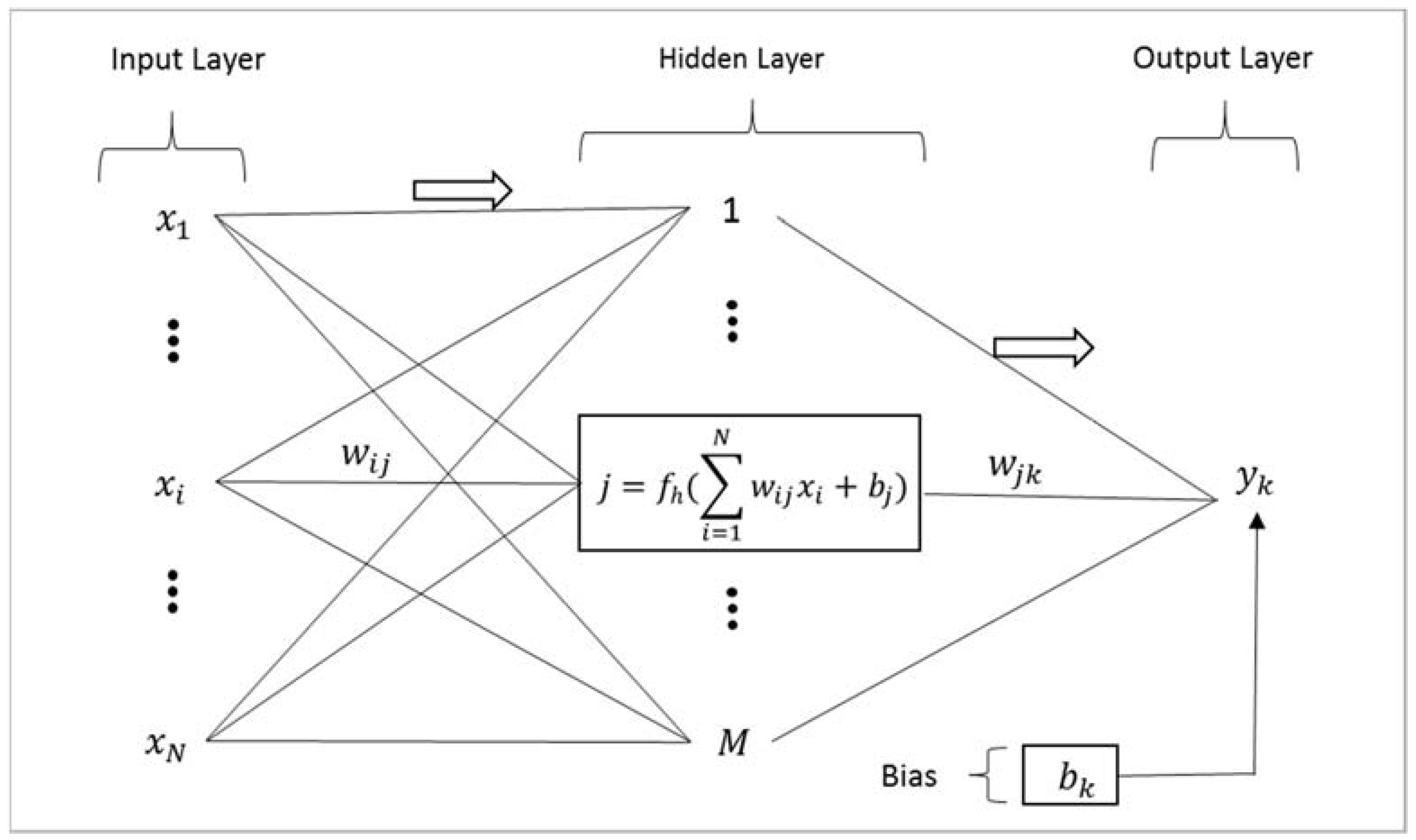
ANNs are one type of soft computing technique with a widespread parallel-distributed information processing system that have performance properties similar to biological neural networks and are able to recognize complex non-linear relationships between input and output vectors [48,49]. ANNs with strong input-output structure have been widely used as a tool in hydrological models [24,50,51,52]. The ANN used in this study is a feed-forward neural network (FFNN) that is the most popular for time series forecasting models [53]. The model is comprised of three layers: the input layer, output layer, and hidden layer (Figure 2). In feed-forward neural networks, neuron connection only occurs from a neuron of the input layer to neurons of the hidden layer and from a neuron of the hidden layer to neurons of the output layer; there is no connection between neurons within one layer. The output value of a three-layered FFNN is expressed as [54]:

$${\mathrm{y}}_{\mathrm{k}}={\mathrm{f}}_{\mathrm{o}}\left[{\displaystyle \sum }_{\mathrm{j}=1}^{\mathrm{M}}{\mathrm{w}}_{\mathrm{jk}}\times {\mathrm{f}}_{\mathrm{h}}({\displaystyle \sum }_{\mathrm{i}=1}^{\mathrm{N}}{\mathrm{w}}_{\mathrm{ij}}{\mathrm{x}}_{\mathrm{i}}+{\mathrm{b}}_{\mathrm{j}})+{\mathrm{b}}_{\mathrm{k}}\right]$$

(1)

where, i, j and k show neurons of input, hidden, and output layers, respectively. ${\mathrm{w}}_{\mathrm{ij}}$ is weight of the ith neuron of input layer connected to the jth neuron of the hidden layer, ${\mathrm{w}}_{\mathrm{jk}}$ is weight of the jth neuron in the hidden layer connected to the kth neuron of the output layer, ${\mathrm{b}}_{\mathrm{j}}$ and ${\mathrm{b}}_{\mathrm{k}}$ are the bias for the $\mathrm{j}$th hidden neuron and the kth output neuron, respectively. ${\mathrm{f}}_{\mathrm{h}}$ and ${\mathrm{f}}_{\mathrm{o}}$ are the activation functions for the hidden and the output neurons, respectively. Activation functions used in this study included a combination of a hyperbolic tangent function (in the hidden layer) and a pure line function (in the output layer) as these functions are effective when extrapolating beyond the range of the training data [55]. ${\mathrm{x}}_{\mathrm{i}}$ is ith input variable, ${\mathrm{y}}_{\mathrm{k}}$ is estimated output variable. $\mathrm{N}$ is the number of the neurons in the input layer that are dependent on the modeled system, and $\mathrm{M}$ is the number of neurons in the hidden layer; in this study, to determine the proper number of neurons in the hidden layer, a trial and error method was used and an optimal ANN structure was selected according to the lowest root mean squared error (RMSE) for the validation phase. The final optimal structure (number of neurons in the input, hidden, and output layers, respectively) are shown in Tables 4–6. A back-propagation mechanism was used to train the network; this algorithm is based on a gradient scheme for weighting adjustment to reduce the error between predicted and observed data. Several variants of the back-propagation training scheme have been developed [56], among these, the Levenberg–Marquardt algorithm is applied in this study. According to the Levenberg–Marquardt algorithm, the weights are adjusted as follows [57]:

$$\Delta \mathrm{W}=-{\left({\mathrm{J}}^{\mathrm{T}}\mathrm{J}+\mathsf{\mu }\mathrm{I}\right)}^{-1}{\mathrm{J}}^{\mathrm{T}}\mathsf{\epsilon }$$

(2)

where, $\mathrm{J}$ is the Jacobian matrix that contains the first derivatives of the network errors relating to the weights and biases, $\mathsf{\epsilon }$ is a vector of network errors, $\mathrm{I}$ is the identity matrix, and $\mathsf{\mu }$ is learning rate with a positive scalar value adjusted at each iteration and governs the relative importance between the Gauss–Newton and gradient descent methods [58]. Details of ANNs and their theoretical foundation can be found in [48].

3.1.1. Determination of Input Structure

In this study, eight scenarios of ANN models, based on the choice of inputs, were considered: (i) using rainfall data; (ii) using rainfall and runoff data; (iii) using rainfall and NDVI; (iv) using rainfall and IC; (v) using rainfall, NDVI, and IC; (vi) using rainfall, runoff, and NDVI; (vii) using rainfall, runoff, and IC; and (viii) using a combination of all parameters rainfall, runoff , NDVI, and IC. To set up current scenarios, statistical parameters, including cross-correlation and partial autocorrelation functions (CCF and PACF, respectively) to avoid trial and error in modelling process were applied to identify significant lag values of inputs [53]. CCF is widely used for input selection in forecasting models, including R-R modelling using data-driven models [59]. We also considered average of monthly rainfall of two previous months as the additional required input, since it had high correlation with runoff data.

3.1.2. Data Pre-Processing

In previous studies, to pre-process data in the ANN model by standardization process, one of these three ranges [0–1], [−1 to +1], or [0.1–0.9] were used. This confining data between specific limits minimizes bias and ensures that they receive the same attention within the network [55]. All input variables in our study were normalized as follows [60] to be in the range [0–1]:

$${\mathrm{X}}_{\mathrm{norm}}=\frac{{\mathrm{X}}_{\mathrm{ori}} {-\mathrm{X}}_{\min }}{{\mathrm{X}}_{\max }{-\mathrm{X}}_{\min }}$$

(3)

where, ${\mathrm{X}}_{\min }$ and ${\mathrm{X}}_{\max }$ represent the minimum and maximum values among original data and ${\mathrm{X}}_{\mathrm{norm}}$ and ${\mathrm{X}}_{\mathrm{ori}}$ represent the normalized and original data, respectively.

3.2. Hydrological Connectivity

The concept of hydrological connectivity is often applied to describe the internal linkages between the sources of runoff and sediment within a catchment to the catchment outlet [61]. Index of Connectivity (IC) is a type of hydrological connectivity index that can be computed in a GIS environment using topography and other catchment characteristics [44]. IC is based on recognized major elements of hydrological connectivity, such as land use as a dynamic element and topographic characteristics as static elements that represents the potential connectivity between different parts of a catchment. The calculation of IC is expressed as follows [44]:

$${\mathrm{IC}=\log }_{10}(\frac{{\mathrm{D}}_{\mathrm{up}}}{{\mathrm{D}}_{\mathrm{dn}}})$$

(4)

where, ${\mathrm{D}}_{\mathrm{up}}$ and ${\mathrm{D}}_{\mathrm{dn}}$ are the upslope and downslope components of connectivity, respectively. IC values range from −∞ to +∞, where larger IC values represent increasing connectivity. The upslope component (${\mathrm{D}}_{\mathrm{up}}$) indicates the potential for downward routing of runoff and sediment and is defined as:

$${\mathrm{D}}_{\mathrm{up}}=\overline{\mathrm{W}}\overline{\mathrm{S}}\sqrt{\mathrm{A}}$$

(5)

where, $\overline{\mathrm{W}}$, $\overline{\mathrm{S}}$ and $\mathrm{A}$ of the upslope contributing area are the average weighting factor (dimensionless), mean slope gradient (m/m), and area (m²), respectively. The downslope component (${\mathrm{D}}_{\mathrm{dn}}$) takes into account the flow path length that a particle travels to arrive at the designated target or sink. Therefore, ${\mathrm{D}}_{\mathrm{dn}}$ can be expressed as:

$${\mathrm{D}}_{\mathrm{dn}}={\displaystyle \sum }_{\mathrm{i}}^{\mathrm{n}}\frac{{\mathrm{d}}_{\mathrm{i}}}{{\mathrm{W}}_{\mathrm{i}}{\mathrm{S}}_{\mathrm{i}}}$$

(6)

where, ${\mathrm{W}}_{\mathrm{i}}$ is the weighting factor of the ith cell, ${\mathrm{S}}_{\mathrm{i}}$ is the slope gradient of the ith cell, and ${\mathrm{d}}_{\mathrm{i}}$ is the length of the ith cell along the downslope direction (m); ${\mathrm{d}}_{\mathrm{i}}$ can assume two values: cell size $\left(\mathrm{l}\right)$ in the case of the main direction and (l√2) in the case of the diagonal direction.

The Hydrologically Enforced Digital Elevation Model (DEM-H) [62] and raster maps of weighting factors with resolutions of 30 × 30 m were applied as the main input data for calculating IC. One of main components of IC is the weighting factor ($\mathrm{W}$) (Equations (5) and (6)). Borselli et al. [44] introduced the weighting factor to model the resistance of each cell against runoff and sediment flow based on characteristics of the local land use and soil surface that were derived from the C-factor of USLE-RUSLE models [63,64]. C-factor values range from 0 to 1, where 0 represents dense vegetation and protected soil and 1 represents bare soil at risk of erosion. However, the same authors note that W should be based on surface features (e.g., roughness index) that influence runoff and sediment processes within a catchment or a hillslope [65]. Considering catchment condition when calculating W provides reasonable results, e.g., differences in the impedance to transport of runoff and sediment in bare areas would not be represented by the C-factor, but better portrayed by a topographic roughness based index. In agricultural and forest environments, describing the impedance to runoff and sediment transport benefits from the application of the C-factor computed based on vegetation cover and land use management data [65]. Therefore, in our two study catchments, applying the C-factor to the weighting factor W is suitable. To estimate the C-factor of USLE-RUSLE, we rescaled NDVI using the following method [66]:

$$\mathrm{W}=\mathrm{C}=(\frac{-\mathrm{NDVI}+1}{2})$$

(7)

where, W is the weighting factor, C is C-factor of USLE-RUSLE and NDVI is Normalized Difference Vegetation Index

3.3. Normalized Difference Vegetation Index

The Normalized Difference Vegetation Index (NDVI) is an indicator of the greenness of vegetation cover, which is widely used for ecosystem monitoring. NDVI is generated from the Near-IR and Red bands of MODIS images as:

$$\mathrm{NDVI}=\frac{\mathrm{NIR}-\mathrm{RED}}{\mathrm{NIR}+\mathrm{RED}}$$

(8)

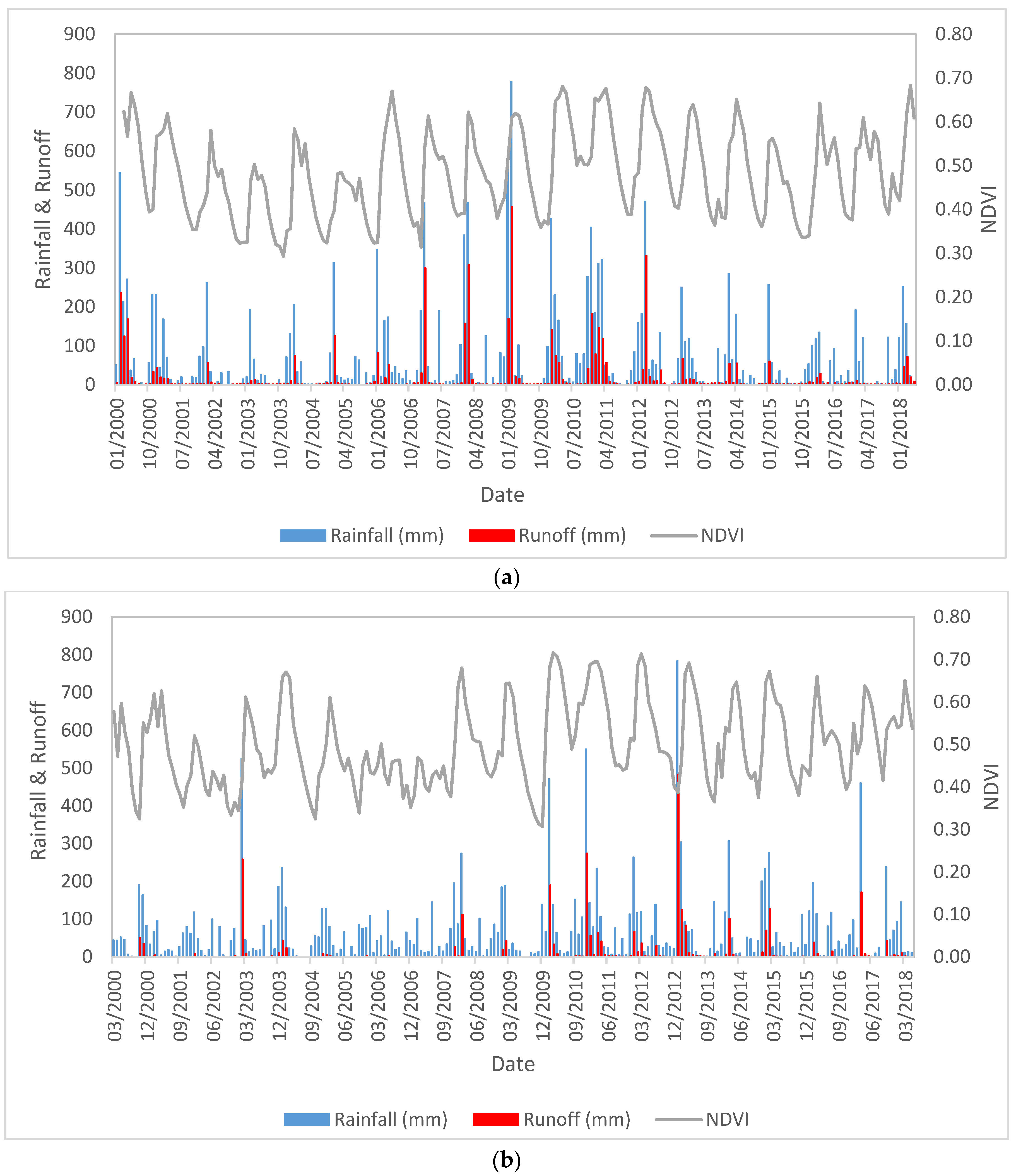
where, NIR and RED are the spectral reflectances measured in the near infrared and red wavebands, respectively. NDVI values range from −1 to 1, where −1 represents bare soil and 1 represents dense vegetation [67]. NDVI values in the two catchments during the period from 2000 to 2018 exhibited temporal variations. Given that the change in NDVI is very low during each month, the NDVI time series values in our study sites were obtained from images in the middle of each month without cloud cover. Investigation of NDVI values showed similar monthly patterns during study years. NDVI values decreased from June, reached a minimum in October or November, and then increased and reached a maximum in February or March in the both catchments (Figure 3a,b).

3.4. Evaluation of Results

We considered three different types of standard statistics to assess the performance of various models during calibration and validation: coefficient of determination (R²), RMSE, and Nash–Sutcliffe model performance coefficient (NS) [60]:

$${\mathrm{R}}^2={\left[\frac{{{\displaystyle \sum }}_{\mathrm{i}=1}^{\mathrm{n}}\left({\mathrm{O}}_{\mathrm{i}}-\overline{\mathrm{O}}\right)\left({\mathrm{S}}_{\mathrm{i}}-\overline{\mathrm{S}}\right)}{\sqrt{{{\displaystyle \sum }}_{\mathrm{i}=1}^{\mathrm{n}}{\left({\mathrm{O}}_{\mathrm{i}}-\overline{\mathrm{O}}\right)}^2}\sqrt{{{\displaystyle \sum }}_{\mathrm{i}=1}^{\mathrm{n}}{\left({\mathrm{S}}_{\mathrm{i}}-\overline{\mathrm{S}}\right)}^2}}\right]}^2$$

(9)

$$\mathrm{RMSE}=\sqrt{\frac{1}{\mathrm{n}}{{\displaystyle \sum }}_{\mathrm{i}=1}^{\mathrm{n}}{\left({\mathrm{O}}_{\mathrm{i}}{-\mathrm{S}}_{\mathrm{i}}\right)}^2}$$

(10)

$$\mathrm{NS}=1-\frac{{{\displaystyle \sum }}_{\mathrm{i}=1}^{\mathrm{i}=\mathrm{n}} {\left({\mathrm{O}}_{\mathrm{i}}{-\mathrm{S}}_{\mathrm{i}}\right)}^2}{{{\displaystyle \sum }}_{\mathrm{i}=1}^{\mathrm{i}=\mathrm{n}} {\left({\mathrm{O}}_{\mathrm{i}}-\overline{\mathrm{O}}\right)}^2}$$

(11)

where, $\mathrm{n}$ is the number of data, ${\mathrm{O}}_{\mathrm{i}}$ and ${\mathrm{S}}_{\mathrm{i}}$ are the ith observed and simulated runoff, respectively, and $\overline{\mathrm{O}}$ and $\overline{\mathrm{S}}$ are the average of observed and simulated runoff, respectively. Higher R² values represent better correlation between simulated and observed values. The RMSE ranges from 0 to +∞, with 0 indicating a perfect fit of the model to observed values. The range of NS values is from −∞ to 1, with a perfect match of simulated and observed values indicated by 1, a value of 0 indicates that simulated data are no better than taking the mean of the observed data, and values <0 indicate very weak model performance. Generally, $\mathrm{NS}>0.6$ is considered as acceptable model performance [50].

4. Results and Discussion

4.1. Statistical Analysis of Data

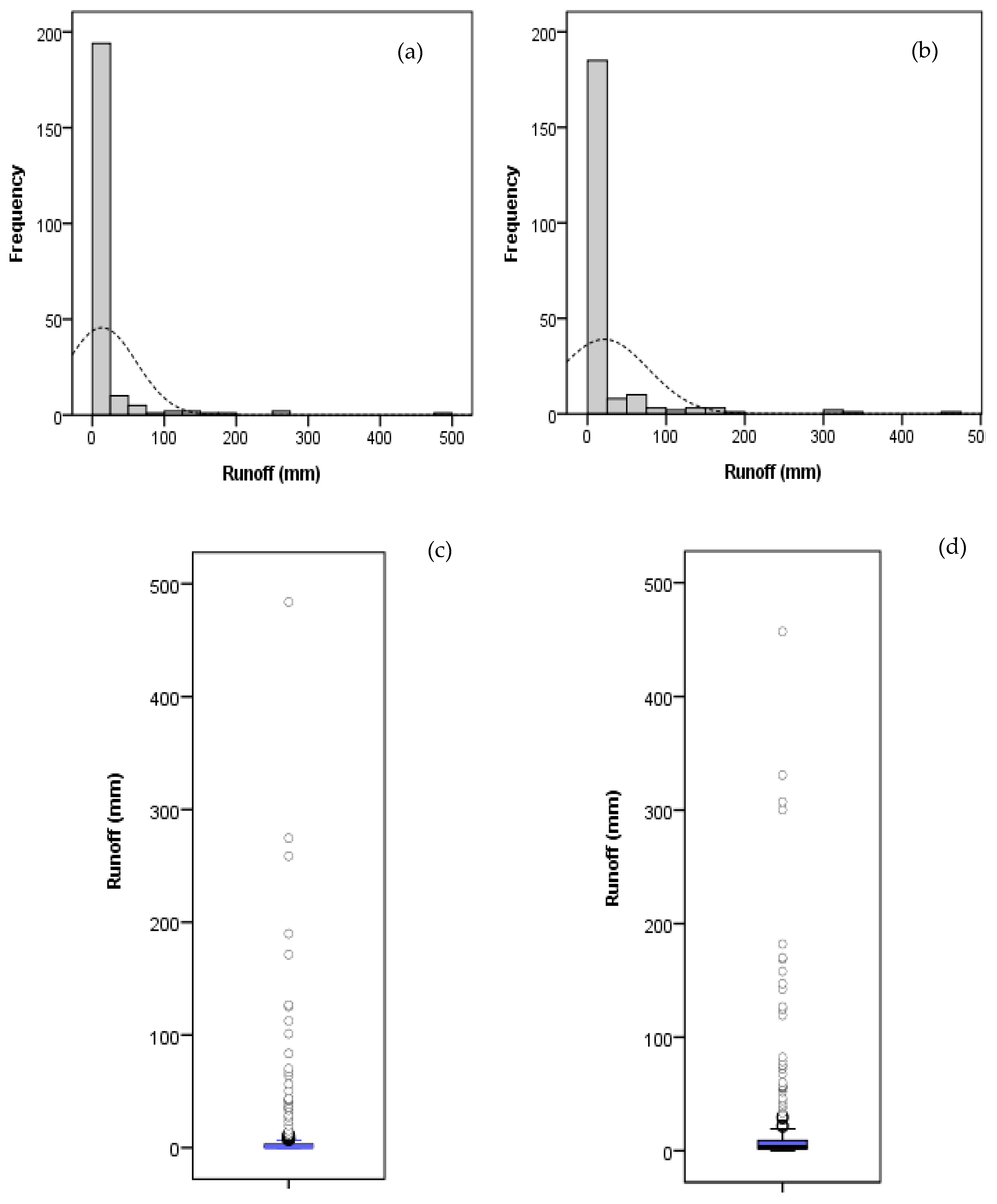
Initially, monthly runoff and rainfall data were surveyed to ensure there were no gaps in the time series, then 70% of the total data were selected for calibration and the remaining 30% were selected for validation for each catchment. The statistical parameters for calibration, validation, and total datasets of rainfall, runoff, NDVI and IC datasets were calculated and are shown in Table 2. For Calliope River (station 132001A), the mean ($\overline{\mathrm{x}})$ and standard deviation ${(\mathsf{\sigma }}_{\mathrm{x}})$ values for the runoff validation datasets were higher than those for the calibration, but for Haughton River (station 119003A), the mean and standard deviation values for runoff validation datasets were less than those for the calibration (Table 2). Furthermore, the coefficient of variation $\left(\mathrm{Cv}\right)$ of the runoff variable for Calliope River is greater than that of Haughton River. Both sites had relatively high values of skewness ${(\mathrm{G}}_1)$ and kurtosis ${(\mathsf{\beta }}_2)$ for both rainfall and runoff variables. Frequency distribution plots in these catchments exhibited non-normal distributions (Figure 4a,b). Based on the runoff box plots (Figure 4c,d), both stations contained several extreme runoff data that, together with the non-normal distribution of data, can affect ANN data-driven models and complicate runoff modelling.

4.2. Development and Application of ANN Model

4.2.1. Results of the Best Input Delay Values

In this study, input selection using CCF was conducted on the training dataset to determine antecedent rainfall values, which had the best correlation with runoff in both catchments. Cross-correlation between monthly runoff and monthly rainfall (with 3-month time lags), revealed that runoff data are highly correlated with rainfall data of the same month, followed by rainfall of the previous month for both catchments (

Table 3. Cross correlation between monthly runoff and rainfall data with 5% significance limits and Partial autocorrelation for monthly runoff data with 5% significance limits for Haughton River and Calliope River catchments.

Catchment	Lag	Cross-Correlation	Partial-Autocorrelation
Haughton River	0	0.88
	1	0.46	0.29
	2	0.11	−0.07
	3	0.00	−0.02
Calliope River	0	0.89
	1	0.17	0.16
	2	0.08	0.02
	3	0.00	−0.03

). We also used the average of monthly rainfall of the two previous months as an input to estimate of runoff, since had high correlation with runoff data. It has also been suggested that using antecedent runoff can improve estimation of runoff values [59]. Partial auto-correlation analysis was also conducted to determine the correlation of runoff in each month with antecedent runoffs in order to select the best lag time with the highest correlation. Results showed that monthly runoff data have the highest correlation coefficient with runoff of the previous month (Table 3).

4.2.2. ANN Models

The ANN models were applied to estimate runoff values using different input sets. Based on CCF and PACF analysis and using rainfall, runoff, NDVI, and IC time series data, 24 input patterns were considered. In all cases, ANN used runoff values of each month as the single output. For all 24 scenarios, simulated runoff was compared with observed runoff based on RMSE, NS, and R². Results of all models are presented in two main sections: in the first section, we present the results of ANN models that used only hydro-climatic data as inputs (

Table 4. Results of monthly time series modelling by Artificial Neural Network (ANN) with hydro-climatic inputs during calibration and validation.

Catchment	Inputs	Structure	Calibration			Validation
			RMSE (mm)	NS	R2	RMSE (mm)	NS	R2
Haughton River	${\mathrm{P}}_t$	1-9-1	25.0	0.94	0.94	10.8	0.71	0.64
	${\mathrm{P}}_{\mathrm{t}}{,\mathrm{P}}_{\mathrm{t}-1}$	2-9-1	22.2	0.95	0.95	10.4	0.73	0.74
	${\mathrm{P}}_{\mathrm{t}},{\overline{\mathrm{P}}}_{\mathrm{t}-1,\mathrm{t}-2}$	2-10-1	21.9	0.96	0.96	9.4	0.79	0.69
	${\mathrm{P}}_{\mathrm{t}}{,\mathrm{R}}_{\mathrm{t}-1}$	2-6-1	16.5	0.94	0.93	9.3	0.79	0.73
	${\mathrm{P}}_{\mathrm{t}}{,\mathrm{P}}_{\mathrm{t}-1}{,\mathrm{R}}_{\mathrm{t}-1}$	3-9-1	17.6	0.90	0.89	9.4	0.78	0.68
	${\mathbf{P}}_{\mathbf{t}}\mathbf{,}{\overline{\mathbf{P}}}_{\mathbf{t}-\mathbf{1}\mathbf{,}\mathbf{t}\mathbf{-}\mathbf{2}}{\mathbf{,}\mathbf{R}}_{\mathbf{t}\mathbf{-}\mathbf{1}}$	3-6-1	15.1	0.97	0.96	9.1	0.80	0.76
Calliope River	${\mathrm{P}}_{\mathrm{t}}$	1-5-1	9.8	0.96	0.96	28.7	0.81	0.81
	${\mathrm{P}}_{\mathrm{t}}{,\mathrm{P}}_{\mathrm{t}-1}$	2-6-1	9.5	0.95	0.96	28.5	0.83	0.82
	${\mathrm{P}}_{\mathrm{t}},{\overline{\mathrm{P}}}_{\mathrm{t}-1,\mathrm{t}-2}$	2-6-1	10.5	0.95	0.94	29.8	0.73	0.74
	${\mathrm{P}}_{\mathrm{t}}{,\mathrm{P}}_{\mathrm{t}-1}$	2-10-1	9.6	0.95	0.96	28.0	0.81	0.81
	${\mathbf{P}}_{\mathbf{t}}{\mathbf{,}\mathbf{P}}_{\mathbf{t}\mathbf{-}\mathbf{1}}{\mathbf{,}\mathbf{R}}_{\mathbf{t}\mathbf{-}\mathbf{1}}$	3-6-1	8.1	0.97	0.97	25.7	0.85	0.85
	$P_t,{\overline{P}}_{t-1,t-2}{,R}_{t-1}$	3-6-1	9.8	0.93	0.96	29.3	0.80	0.80

${\mathrm{P}}_{\mathrm{t}}$: Rainfall value of the (t)th month, ${\mathrm{P}}_{\mathrm{t}-1}$: Rainfall value of the (t−1)th month, ${\overline{\mathrm{P}}}_{\mathrm{t}-1,\mathrm{t}-2}$: Average of monthly rainfall value of the (t−1)th and (t−2)th months and ${\mathrm{R}}_{\mathrm{t}-1}$: Runoff value of the (t−1)th month.

) and in the second section, results of the combination of hydro-climatic inputs with IC, NDVI, and both NDVI and IC are presented for Haughton River and Calliope River (

Table 5. Results of monthly time series modelling by ANN with different inputs during calibration and validation in the Haughton River catchment.

Inputs	Structure	Calibration			Validation
		RMSE (mm)	NS	R2	RMSE (mm)	NS	R2
${\mathrm{P}}_{\mathrm{t}}{,\mathrm{NDVI}}_{\mathrm{t}}$	2-6-1	13.6	0.98	0.96	9.1	0.80	0.76
${\mathrm{P}}_{\mathrm{t}}{,\mathrm{P}}_{\mathrm{t}-1}{,\mathrm{NDVI}}_{\mathrm{t}}$	3-10-1	8.3	0.99	0.99	7.7	0.85	0.79
${\mathrm{P}}_{\mathrm{t}}{,\overline{\mathrm{P}}}_{\mathrm{t}-1,\mathrm{t}-2}{,\mathrm{NDVI}}_{\mathrm{t}}$	3-6-1	15.1	0.97	0.95	7.8	0.85	0.79
${\mathbf{P}}_{\mathbf{t}}{\mathbf{,}\mathbf{IC}}_{\mathbf{t}}$	2-10-1	12.5	0.98	0.96	7.2	0.87	0.82
${\mathrm{P}}_{\mathrm{t}}{,\mathrm{P}}_{\mathrm{t}-1}{,\mathrm{IC}}_{\mathrm{t}}$	3-11-1	12.1	0.98	0.97	7.4	0.87	0.81
${\mathrm{P}}_{\mathrm{t}}{,\overline{\mathrm{P}}}_{\mathrm{t}-1,\mathrm{t}-2}{,\mathrm{IC}}_{\mathrm{t}}$	3-5-1	14.8	0.97	0.95	7.4	0.87	0.81
${\mathrm{P}}_{\mathrm{t}}{,\mathrm{NDVI}}_{\mathrm{t}}{,\mathrm{IC}}_{\mathrm{t}}$	3-9-1	14.7	0.97	0.96	8.2	0.84	0.76
${\mathrm{P}}_{\mathrm{t}}{,\mathrm{P}}_{\mathrm{t}-1}{,\mathrm{NDVI}}_{\mathrm{t}}{,\mathrm{IC}}_{\mathrm{t}}$	4-10-1	14.2	0.97	0.97	8.4	0.83	0.75
${\mathrm{P}}_{\mathrm{t}}{,\overline{\mathrm{P}}}_{\mathrm{t}-1,\mathrm{t}-2}{,\mathrm{NDVI}}_{\mathrm{t}}{,\mathrm{IC}}_{\mathrm{t}}$	4-10-1	19.2	0.95	0.93	10.1	0.75	0.71
${\mathrm{P}}_{\mathrm{t}}{,\mathrm{R}}_{\mathrm{t}-1}{,\mathrm{NDVI}}_{\mathrm{t}}$	3-6-1	14.8	0.97	0.96	8.4	0.83	0.79
${\mathrm{P}}_{\mathrm{t}}{,\mathrm{P}}_{\mathrm{t}-1}{,\mathrm{R}}_{\mathrm{t}-1}{,\mathrm{NDVI}}_{\mathrm{t}}$	4-11-1	19.8	0.95	0.93	9.7	0.77	0.74
${\mathrm{P}}_{\mathrm{t}}{,\overline{\mathrm{P}}}_{\mathrm{t}-1,\mathrm{t}-2}{,\mathrm{R}}_{\mathrm{t}-1}{,\mathrm{NDVI}}_{\mathrm{t}}$	4-11-1	14.4	0.97	0.95	8.9	0.81	0.73
${\mathrm{P}}_{\mathrm{t}}{,\mathrm{R}}_{\mathrm{t}-1}{,\mathrm{IC}}_{\mathrm{t}}$	3-6-1	16.3	0.97	0.95	8.2	0.84	0.76
${\mathrm{P}}_{\mathrm{t}}{,\mathrm{P}}_{\mathrm{t}-1}{,\mathrm{R}}_{\mathrm{t}-1}{,\mathrm{IC}}_{\mathrm{t}}$	4-6-1	15.7	0.97	0.97	8.5	0.82	0.79
${\mathrm{P}}_{\mathrm{t}}{,\overline{\mathrm{P}}}_{\mathrm{t}-1,\mathrm{t}-2}{,\mathrm{R}}_{\mathrm{t}-1}{,\mathrm{IC}}_{\mathrm{t}}$	4-6-1	13.7	0.98	0.96	8.3	0.83	0.81
${\mathrm{P}}_{\mathrm{t}}{,\mathrm{R}}_{\mathrm{t}-1}{,\mathrm{NDVI}}_{\mathrm{t}}{,\mathrm{IC}}_{\mathrm{t}}$	4-6-1	19.7	0.95	0.93	7.5	0.86	0.80
${\mathrm{P}}_{\mathrm{t}}{,\mathrm{P}}_{\mathrm{t}-1}{,\mathrm{R}}_{\mathrm{t}-1}{,\mathrm{NDVI}}_{\mathrm{t}}{,\mathrm{IC}}_{\mathrm{t}}$	5-5-1	17.4	0.96	0.95	8.2	0.83	0.76
${\mathrm{P}}_{\mathrm{t}}{,\overline{\mathrm{P}}}_{\mathrm{t}-1,\mathrm{t}-2}{,\mathrm{R}}_{\mathrm{t}-1}{,\mathrm{NDVI}}_{\mathrm{t}}{,\mathrm{IC}}_{\mathrm{t}}$	5-6-1	14.4	0.97	0.95	8.3	0.83	0.77

and

Table 6. Results of monthly time series modelling by ANN with different inputs during calibration and validation in the Calliope River catchment.

Inputs	Structure	Calibration			Validation
		RMSE (mm)	NS	R2	RMSE (mm)	NS	R2
${\mathrm{P}}_{\mathrm{t}}{,\mathrm{NDVI}}_{\mathrm{t}}$	2-10-1	9.3	0.96	0.92	19.0	0.92	0.93
${\mathrm{P}}_{\mathrm{t}}{,\mathrm{P}}_{\mathrm{t}-1}{,\mathrm{NDVI}}_{\mathrm{t}}$	3-7-1	8.8	0.96	0.96	25.6	0.85	0.88
${\mathrm{P}}_{\mathrm{t}}{,\overline{\mathrm{P}}}_{\mathrm{t}-1,\mathrm{t}-2}{,\mathrm{NDVI}}_{\mathrm{t}}$	3-6-1	7.8	0.969	0.95	29.0	0.81	0.89
${\mathrm{P}}_{\mathrm{t}}{,\mathrm{IC}}_{\mathrm{t}}$	2-10-1	8.6	0.96	0.95	18.8	0.92	0.92
${\mathrm{P}}_{\mathrm{t}}{,\mathrm{P}}_{\mathrm{t}-1}{,\mathrm{IC}}_{\mathrm{t}}$	3-9-1	6.2	0.98	0.97	20.9	0.90	0.92
${\mathrm{P}}_{\mathrm{t}}{,\overline{\mathrm{P}}}_{\mathrm{t}-1,\mathrm{t}-2}{,\mathrm{IC}}_{\mathrm{t}}$	3-10-1	5.8	0.98	0.94	23.6	0.87	0.88
${\mathrm{P}}_{\mathrm{t}}{,\mathrm{NDVI}}_{\mathrm{t}}{,\mathrm{IC}}_{\mathrm{t}}$	3-11-1	8.2	0.97	0.97	18.5	0.94	0.96
${\mathrm{P}}_{\mathrm{t}}{,\mathrm{P}}_{\mathrm{t}-1}{,\mathrm{NDVI}}_{\mathrm{t}}{,\mathrm{IC}}_{\mathrm{t}}$	4-11-1	6.4	0.98	0.97	22.7	0.88	0.88
${\mathrm{P}}_{\mathrm{t}}{,\overline{\mathrm{P}}}_{\mathrm{t}-1,\mathrm{t}-2}{,\mathrm{NDVI}}_{\mathrm{t}}{,\mathrm{IC}}_{\mathrm{t}}$	4-7-1	13.5	0.91	0.94	19.0	0.92	0.92
${\mathrm{P}}_{\mathrm{t}}{,\mathrm{R}}_{\mathrm{t}-1}{,\mathrm{NDVI}}_{\mathrm{t}}$	3-7-1	6.5	0.98	0.98	26.5	0.84	0.86
${\mathrm{P}}_{\mathrm{t}}{,\mathrm{P}}_{\mathrm{t}-1}{,\mathrm{R}}_{\mathrm{t}-1}{,\mathrm{NDVI}}_{\mathrm{t}}$	4-11-1	6.4	0.98	0.95	27.6	0.83	0.83
${\mathrm{P}}_{\mathrm{t}}{,\overline{\mathrm{P}}}_{\mathrm{t}-1,\mathrm{t}-2}{,\mathrm{R}}_{\mathrm{t}-1}{,\mathrm{NDVI}}_{\mathrm{t}}$	4-6-1	6.8	0.98	0.98	24.1	0.87	0.88
${\mathbf{P}}_{\mathbf{t}}{\mathbf{,}\mathbf{R}}_{\mathbf{t}\mathbf{-}\mathbf{1}}{\mathbf{,}\mathbf{IC}}_{\mathbf{t}}$	3-11-1	6.1	0.98	0.99	18.0	0.95	0.96
${\mathrm{P}}_{\mathrm{t}}{,\mathrm{P}}_{\mathrm{t}-1}{,\mathrm{R}}_{\mathrm{t}-1}{,\mathrm{IC}}_{\mathrm{t}}$	4-10-1	6.4	0.98	0.97	18.4	0.92	0.93
${\mathrm{P}}_{\mathrm{t}}{,\overline{\mathrm{P}}}_{\mathrm{t}-1,\mathrm{t}-2}{,\mathrm{R}}_{\mathrm{t}-1}{,\mathrm{IC}}_{\mathrm{t}}$	4-7-1	9.5	0.95	0.96	23.6	0.87	0.87
${\mathrm{P}}_{\mathrm{t}}{,\mathrm{R}}_{\mathrm{t}-1}{,\mathrm{NDVI}}_{\mathrm{t}}{,\mathrm{IC}}_{\mathrm{t}}$	4-10-1	6.6	0.98	0.98	22.3	0.89	0.91
${\mathrm{P}}_{\mathrm{t}}{,\mathrm{P}}_{\mathrm{t}-1}{,\mathrm{R}}_{\mathrm{t}-1}{,\mathrm{NDVI}}_{\mathrm{t}}{,\mathrm{IC}}_{\mathrm{t}}$	5-6-1	10.5	0.94	0.95	27.9	0.82	0.86
${\mathrm{P}}_{\mathrm{t}}{,\overline{\mathrm{P}}}_{\mathrm{t}-1,\mathrm{t}-2}{,\mathrm{R}}_{\mathrm{t}-1}{,\mathrm{NDVI}}_{\mathrm{t}}{,\mathrm{IC}}_{\mathrm{t}}$	5-10-1	8.6	0.96	0.97	28.4	0.75	0.74

).

Different Patterns of Hydro-Climate Data

Here we analyzed two different patterns of hydro-climate data as ANN inputs: (i) rainfall data and (ii) a combination of rainfall and runoff data. Based on RMSE, NS, and R², the best input pattern in first group was ${\mathrm{P}}_{\mathrm{t}}\mathrm{and}{\overline{\mathrm{P}}}_{\mathrm{t}-1,\mathrm{t}-2}$ for Haughton River and ${\mathrm{P}}_{\mathrm{t}}{\mathrm{and}\mathrm{P}}_{\mathrm{t}-1}$ for Calliope River. In the second group, ${\mathrm{P}}_{\mathrm{t}}{,\overline{\mathrm{P}}}_{\mathrm{t}-1,\mathrm{t}-2}{\mathrm{and}\mathrm{R}}_{\mathrm{t}-1}$ was the best model for Haughton River and ${\mathrm{P}}_{\mathrm{t}}{,\mathrm{P}}_{\mathrm{t}-1}{\mathrm{and}\mathrm{R}}_{\mathrm{t}-1}$ for Calliope River (Table 4). Overall, results showed that for both catchments, including rainfall of the previous months increased model accuracy compared to just using rainfall of the same month. This shows the importance of antecedent soil moisture in the runoff generation process [68]. Additionally, including runoff and rainfall together as input data slightly improved model performance for both catchments (Table 4), indicating that only using rainfall is insufficient to precisely estimate runoff, while combining this with antecedent runoff improves predictions [59].

Combination of Hydro-Climate, Hydro-Geomorphic and Biophysical Data

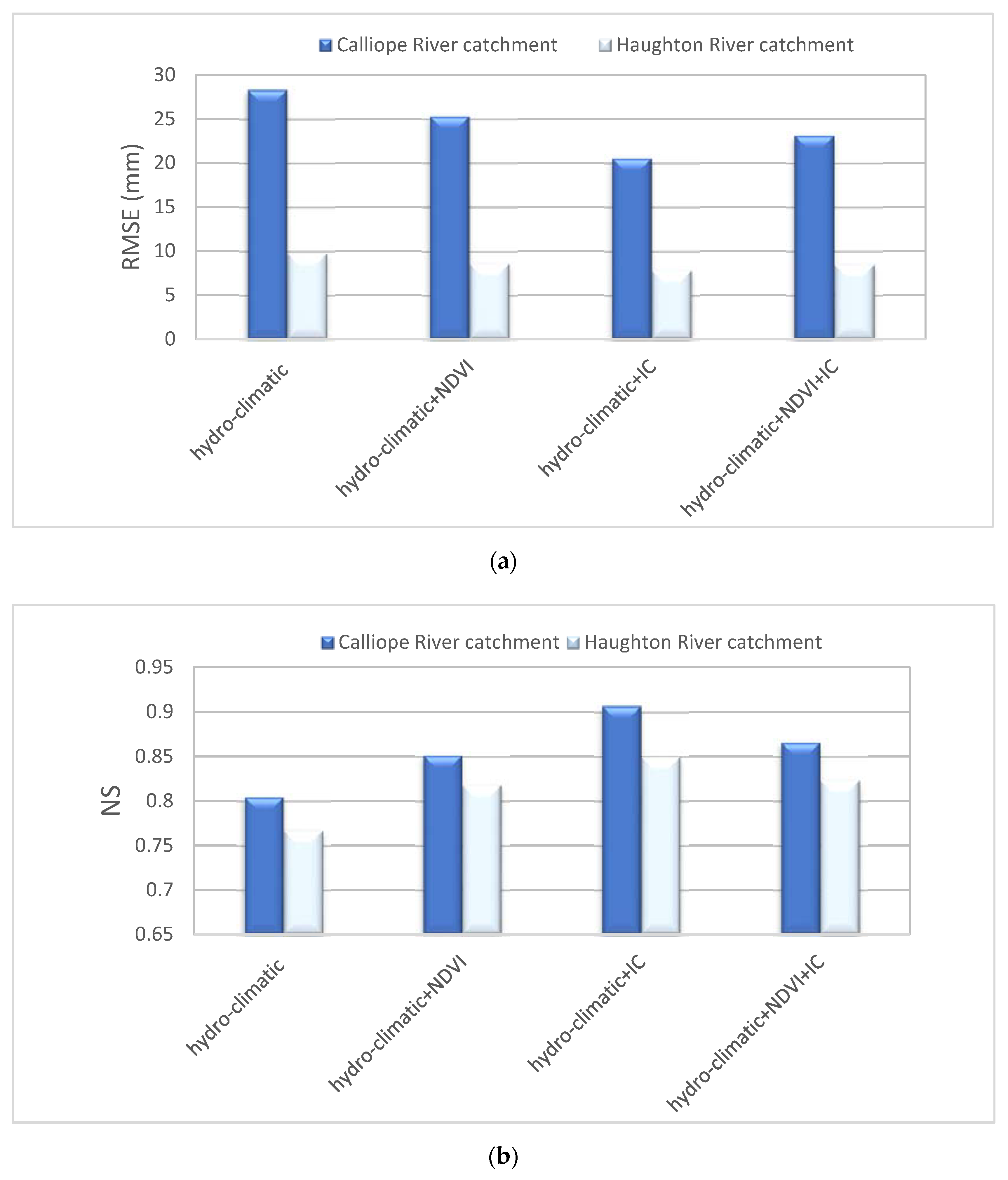
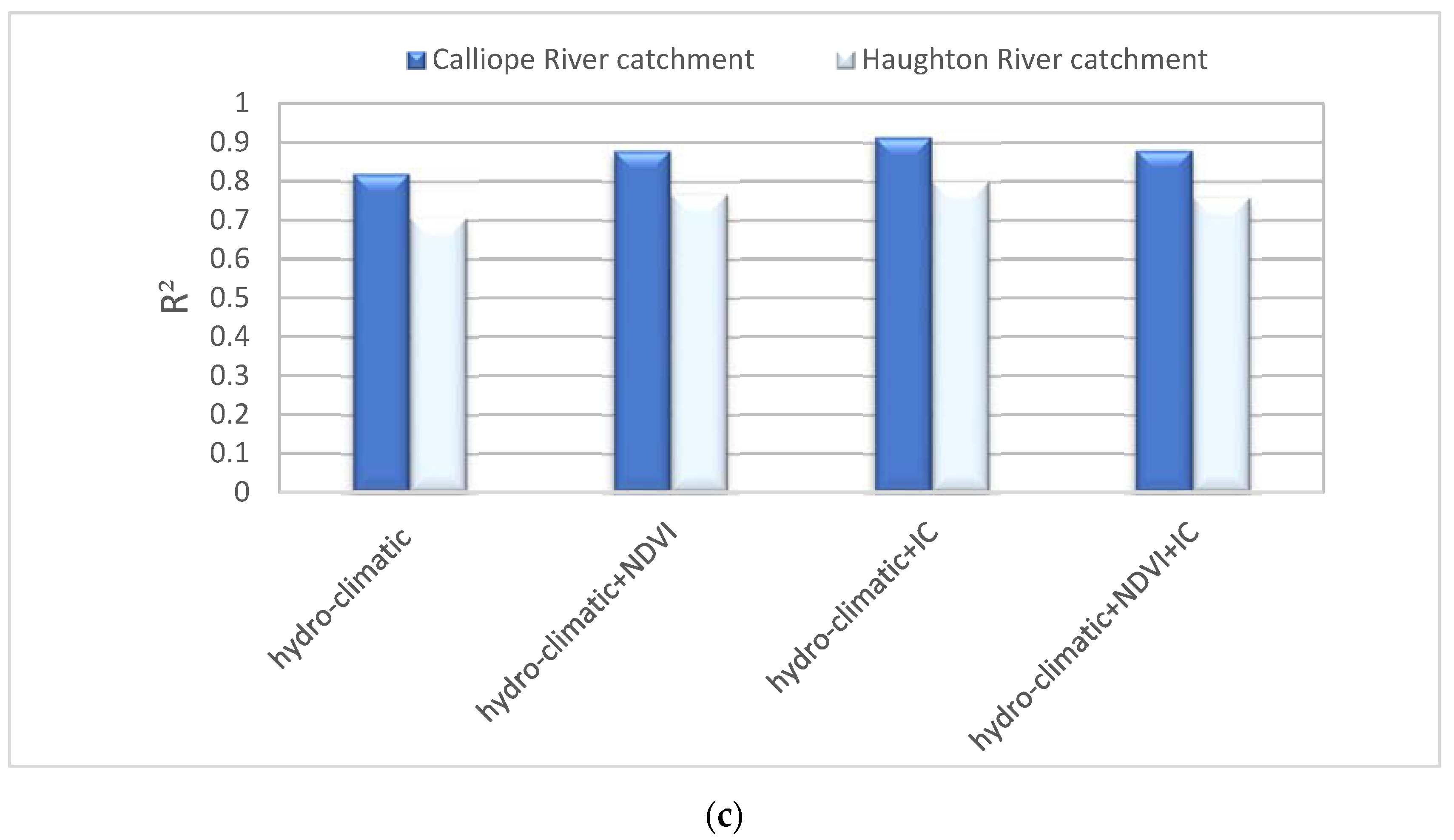
To better evaluate all 24 ANN models with different inputs, average of performance indices (RMSE, NS, and R²) for models using only hydro-climatic inputs (Table 4) and models using combinations of hydro-climatic data (P and R), hydro-geomorphic (IC) and biophysical data (NDVI) (Table 5 and Table 6) were computed and presented separately for Haughton River and Calliope River (Figure 5a–c). Evaluation of results (compared to models using only hydro-climatic inputs) showed that for Haughton River catchment, IC as the model input, improved NS by 9.77%, R² by 11.76%, and decreased RMSE by 24.43%; NDVI as the model input, improved NS by 6.24%, R² by 8.08%, and decreased RMSE by 13.22%; and NDVI together with IC as model inputs, improved NS by 6.92%, R² by 6.86%, and decreased RMSE by 14.98%. For Calliope River catchment, IC improved NS by 11.25%, R² by 10.29%, and decreased RMSE by 37.89%; NDVI improved NS by 5.52%, R² by 6.72%, and decreased RMSE by 11.89%; and NDVI along with IC, improved NS by 7.05%, R² by 6.93%, and decreased RMSE by 22.48%. Comparison amongst different input patterns showed that IC inputs can better improve the performance of models compared to NDVI inputs in both catchments and the best input patterns during the validation phase based on RMSE, NS and R² were ${\mathrm{P}}_{\mathrm{t}}{\mathrm{and}\mathrm{IC}}_{\mathrm{t}}$ for Haughton River and ${\mathrm{P}}_{\mathrm{t}}{,\mathrm{R}}_{\mathrm{t}-1}{\mathrm{and}\mathrm{IC}}_{\mathrm{t}}$ for Calliope River. On the other hand, NDVI together with IC as model inputs improved the prediction results, but ANN performance is lower compared to using only IC data. These results may be explained by the fact that, since NDVI data was used to compute IC, thus NDVI together with IC input nodes increase the network complexity, without offering information that is essential for the modelling. Overall, our comparisons amongst ANN models showed that combining hydro-climatic data with IC and NDVI produced better results (higher NS and R² values and smaller RMSE) than models using only hydro-climatic data. These results demonstrate that runoff characteristics are affected by hydro-geomorphic features [47], biophysical data [69] and in general, incorporating catchment geomorphological characteristics within ANN model elevate the performance of R-R modelling [27,42,43].

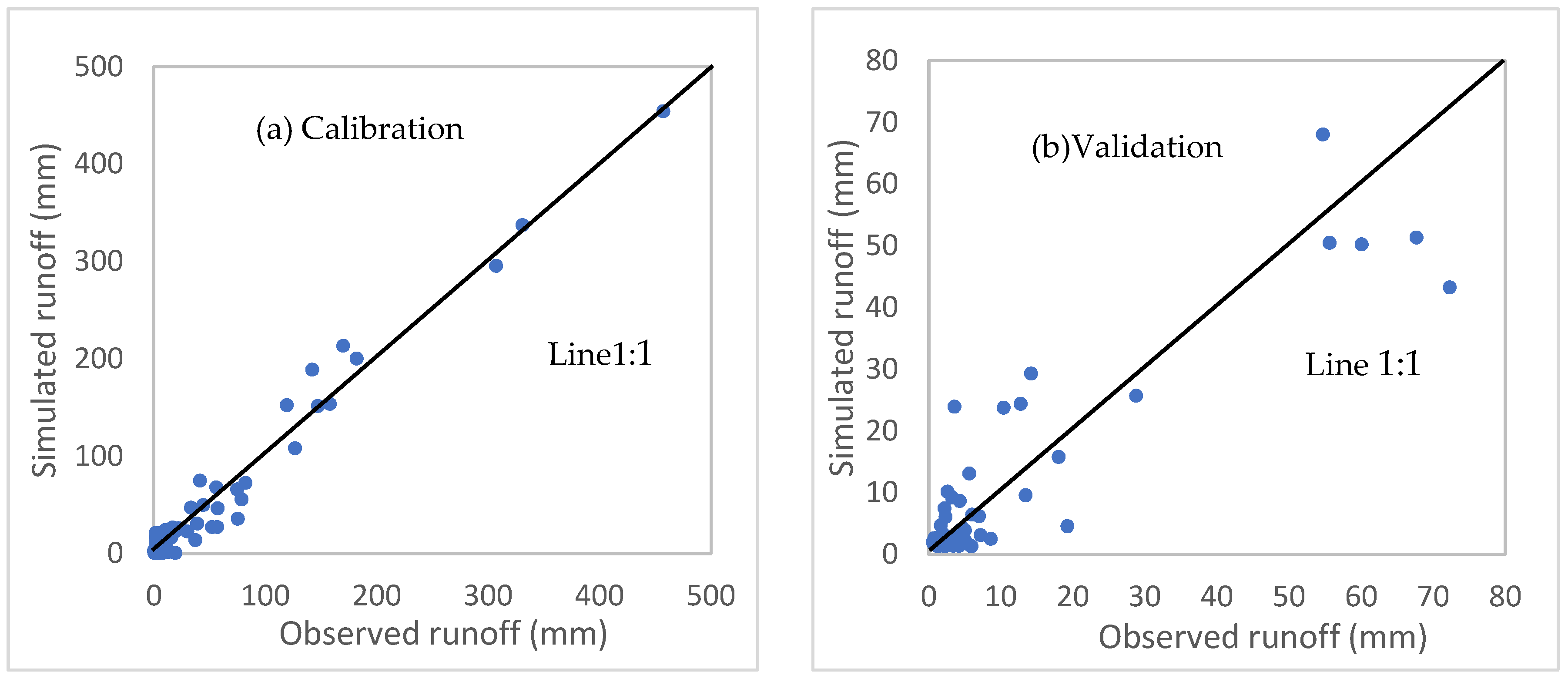
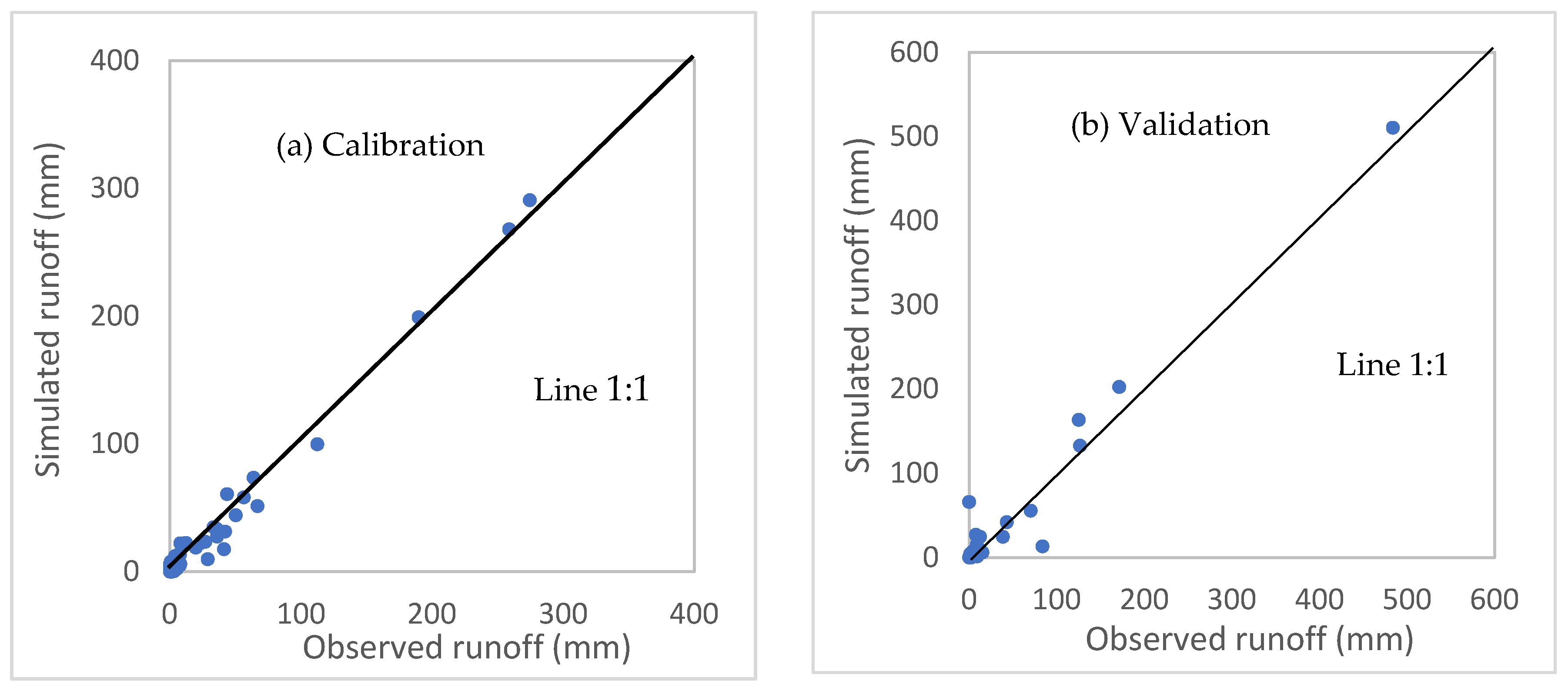
Comparing the calibration with the validation phase revealed that, in Calliope River, the performance indices values of the ANN models during the calibration phase were better than those during the validation phase, while in Haughton River this was reverse. This result based on the statistical parameters (Table 2) is understandable. For both the calibration and validation phases, scatter plots are presented for the best input patterns of ANN models (bold type in Table 5 and Table 6) for the Haughton River catchment (Figure 6) and Calliope River catchment (Figure 7). Comparison of scatter plots between observed and simulated runoff data for two catchments showed that observed runoff during the validation period in Haughton River spanned a wider range than these values in Calliope River. Additionally, simulated runoff values for Calliope River were in closer agreement with the observed values (calibration: R² = 0.99, validation: R² = 0.96), than those for Haughton River (calibration: R² = 0.96, validation: R² = 0.82).

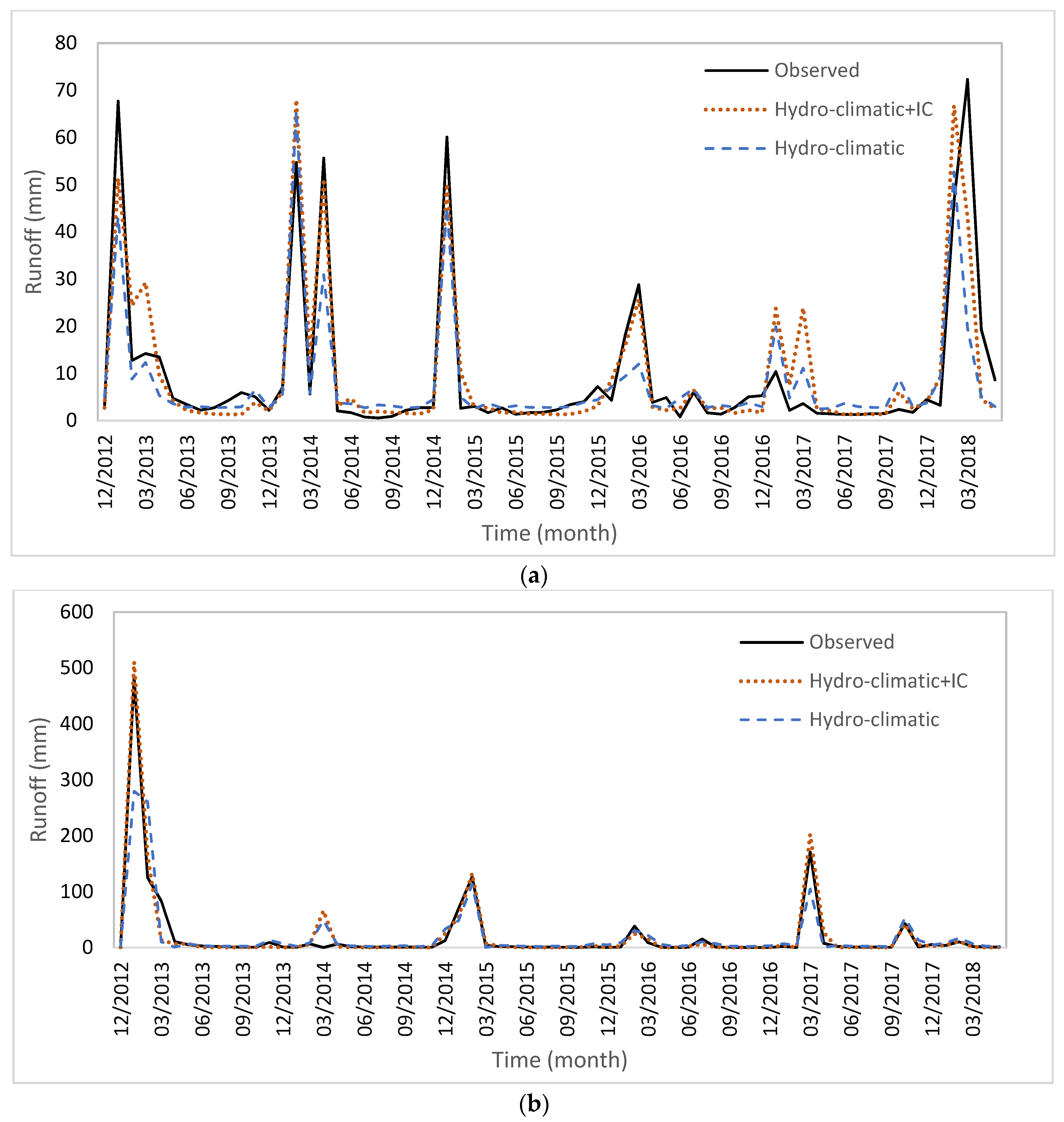
Moreover, plots of temporal variations of observed runoff versus simulated runoff of the best model using only hydro-climatic inputs (${\mathrm{P}}_{\mathrm{t}}, {\overline{\mathrm{P}}}_{\mathrm{t}-1,\mathrm{t}-2}{\mathrm{and}\mathrm{R}}_{\mathrm{t}-1}$ for Haughton River and ${\mathrm{P}}_{\mathrm{t}}{,\mathrm{P}}_{\mathrm{t}-1}{\mathrm{and}\mathrm{R}}_{\mathrm{t}-1}$ for Calliope River) and simulated runoff of the best model using a combination of hydro-climatic inputs with new inputs (${\mathrm{P}}_{\mathrm{t}}{\mathrm{and}\mathrm{IC}}_{\mathrm{t}}$ for Haughton River and ${\mathrm{P}}_{\mathrm{t}}{,\mathrm{R}}_{\mathrm{t}-1}{\mathrm{and}\mathrm{IC}}_{\mathrm{t}}$ for Calliope River) are shown in Figure 8a,b for Haughton and Calliope Rivers, respectively. These graphs confirm the agreement between observed and simulated runoff values during the validation period when IC is used along with hydro-climatic inputs, particularly for Calliope River.

Additionally, to evaluate the ability of model in addition to goodness of fit, accurate prediction of peak runoff values is also important. In this regard, relative error in simulating peak runoff ${(\%\mathrm{RE}}_{\mathrm{P}})$ for the best model using only hydro-climatic inputs and the best model using hydro-climatic inputs along with new inputs was calculated according to the following equation [27] and the results are presented in

Table 7. Assessment of models based on relative error in peak runoff for the best model using only hydro-climatic inputs and the best model using hydro-climatic inputs along with new inputs for Haughton River and Calliope River catchments.

Input Pattern	Haughton River		Calliope River
	The Best Model	%REp	The Best Model	%REp
Hydro-climatic	${\mathrm{P}}_{\mathrm{t}},{\overline{\mathrm{P}}}_{\mathrm{t}-1,\mathrm{t}-2}{,\mathrm{R}}_{\mathrm{t}-1}$	−36.1	${\mathrm{P}}_{\mathrm{t}}{,\mathrm{P}}_{\mathrm{t}-1}{,\mathrm{R}}_{\mathrm{t}-1}$	−17.9
Hydro-climatic + IC	${\mathrm{P}}_{\mathrm{t}}{,\mathrm{IC}}_{\mathrm{t}}$	−12.8	${\mathrm{P}}_{\mathrm{t}}{,\mathrm{R}}_{\mathrm{t}-1}{,\mathrm{IC}}_{\mathrm{t}}$	−3.9
Hydro-climatic + NDVI	${\mathrm{P}}_{\mathrm{t}}{,\mathrm{P}}_{\mathrm{t}-1}{,\mathrm{NDVI}}_{\mathrm{t}}$	−14.0	${\mathrm{P}}_{\mathrm{t}}{,\mathrm{NDVI}}_{\mathrm{t}}$	−16.4
Hydro-climatic + NDVI+IC	${\mathrm{P}}_{\mathrm{t}}{,\mathrm{R}}_{\mathrm{t}-1}{,\mathrm{NDVI}}_{\mathrm{t}}{,\mathrm{IC}}_{\mathrm{t}}$	–15.6	${\mathrm{P}}_{\mathrm{t}}{,\mathrm{NDVI}}_{\mathrm{t}}{,\mathrm{IC}}_{\mathrm{t}}$	−22.3

.

$${\%\mathrm{RE}}_{\mathrm{P}}=\frac{{\mathrm{S}}_{\mathrm{P}}-{\mathrm{O}}_{\mathrm{P}}}{{\mathrm{O}}_{\mathrm{P}}}\times 100$$

(12)

where, ${\mathrm{O}}_{\mathrm{P}}$ and ${\mathrm{S}}_{\mathrm{P}}$ are the observed and simulated peak runoff, respectively. The results indicated that, in general, peak runoff values were simulated more accurately when adding IC to hydro-climatic inputs, in the both catchments, especially in Calliope River catchment.

5. Conclusions

This study was designed to improve R-R modelling using different input patterns in ANN data-driven models for two catchments in Queensland, Australia. Our objective was to examine the most effective and accessible model input variables based on hydrologic understanding to achieve better estimates of monthly runoff. To accomplish this goal, we investigated the effects of NDVI as a biophysical input and IC as a hydro-geomorphic input, along with rainfall and runoff as hydro-climatic inputs on modelling performance. This study concluded the significant effect of IC and NDVI time series inputs for estimating monthly runoff using ANN models. Combining catchment geomorphic and biophysical parameters as a single parameter (IC in this case) not only reduced the number of model parameters, also increased accuracy of the model simulations by a slight increase (9.77% and 11.25%) in the Nash–Sutcliffe efficiency and noticeable decrease (24.43% and 37.89%) in the root mean squared error of monthly runoff from Haughton River and Calliope River, respectively. We also concluded that remote sensing can provide spatially explicit information from catchment conditions. This dynamic information from catchment such as land cover can be used in data-driven models to increase the model performance. These improvements in runoff predictions are valuable for water resources planning and management. Although our results showed that IC is a promising and reliable input within ANN models for better simulating R-R processes, however, more research is required to evaluate the efficiency of these inputs in other scenarios, such as simulation of event-based R-R, simulation of sediment transport, modelling using other artificial intelligence models (e.g., ANFIS, SVR), and application in other catchments. Given that the use of high quality data in data-driven models will lead to more reliable results, input data preparation is important for such studies. Availability of the reliable hydro-climatic data is one of the limitations of these kind of models. Moreover, availability of remotely-sensed land cover datasets (i.e., NDVI) and high resolution topographic data to represent catchment geomorphic characteristics, can also be a limiting factor. For example, availability of cloud-free satellite data that can present spatial and temporal dynamics of vegetation cover in catchment, is critical in deriving NDVI and IC parameters.

References

- Srinivasulu, S.; Jain, A. A comparative analysis of training methods for artificial neural network rainfall–runoff models. Appl. Soft Comput. 2006, 6, 295–306. [Google Scholar] [CrossRef]
- Porporato, A.; Ridolfi, L. Multivariate nonlinear prediction of river flows. J. Hydrol. 2001, 248, 109–122. [Google Scholar] [CrossRef]
- Pumo, D.; Viola, F.; Noto, L.V. Generation of natural runoff monthly series at ungauged sites using a regional regressive model. Water 2016, 8, 209. [Google Scholar] [CrossRef]
- Pumo, D.; Conti, F.L.; Viola, F.; Noto, L.V. An automatic tool for reconstructing monthly time-series of hydro-climatic variables at ungauged basins. Environ. Model. Softw. 2017, 95, 381–400. [Google Scholar] [CrossRef]
- Grayson, R.B.; Moore, I.D.; McMahon, T.A. Physically based hydrologic modeling: 1. A terrain-based model for investigative purposes. Water Resour. Res. 1992, 28, 2639–2658. [Google Scholar] [CrossRef]
- Tiwari, H.; Rai, S. Review of Information and soft computing techniques (ISCT) approaches in Water Resources Projects. In Managing Information Technology; DESIDOC: Delhi, India, 2015; pp. 89–94. [Google Scholar]
- Antar, M.A.; Elassiouti, I.; Allam, M.N. Rainfall-runoff modelling using artificial neural networks technique: A Blue Nile catchment case study. Hydrol. Process. 2006, 20, 1201–1216. [Google Scholar] [CrossRef]
- Jain, A.; Sudheer, K.; Srinivasulu, S. Identification of physical processes inherent in artificial neural network rainfall runoff models. Hydrol. Process. 2004, 18, 571–581. [Google Scholar] [CrossRef]
- Lallahem, S.; Mania, J. A nonlinear rainfall-runoff model using neural network technique: Example in fractured porous media. Math. Comput. Model. 2003, 37, 1047–1061. [Google Scholar] [CrossRef]
- Nourani, V. An emotional ANN (EANN) approach to modeling rainfall-runoff process. J. Hydrol. 2017, 544, 267–277. [Google Scholar] [CrossRef]
- Nourani, V.; Kalantari, O. Integrated artificial neural network for spatiotemporal modeling of rainfall–runoff–sediment processes. Environ. Eng. Sci. 2010, 27, 411–422. [Google Scholar] [CrossRef]
- Phukoetphim, P.; Shamseldin, A.Y.; Adams, K. Multimodel approach using neural networks and symbolic regression to combine the estimated discharges of rainfall-runoff models. J. Hydrol. Eng. 2016, 21, 04016022. [Google Scholar] [CrossRef]
- Tongal, H.; Booij, M.J. Simulation and forecasting of streamflows using machine learning models coupled with base flow separation. J. Hydrol. 2018, 564, 266–282. [Google Scholar] [CrossRef]
- Wilby, R.; Abrahart, R.; Dawson, C. Detection of conceptual model rainfall—Runoff processes inside an artificial neural network. Hydrol. Sci. J. 2003, 48, 163–181. [Google Scholar] [CrossRef]
- Wu, C.; Chau, K. Rainfall–runoff modeling using artificial neural network coupled with singular spectrum analysis. J. Hydrol. 2011, 399, 394–409. [Google Scholar] [CrossRef] [Green Version]
- Hsu, K.l.; Gupta, H.V.; Sorooshian, S. Artificial neural network modeling of the rainfall-runoff process. Water Resour. Res. 1995, 31, 2517–2530. [Google Scholar] [CrossRef]
- Birikundavyi, S.; Labib, R.; Trung, H.T.; Rousselle, J. Performance of neural networks in daily streamflow forecasting. J. Hydrol. Eng. 2002, 7, 392–398. [Google Scholar] [CrossRef]
- Lin, J.-Y.; Cheng, C.-T.; Chau, K.-W. Using support vector machines for long-term discharge prediction. Hydrol. Sci. J. 2006, 51, 599–612. [Google Scholar] [CrossRef] [Green Version]
- Lohani, A.K.; Goel, N.; Bhatia, K. Comparative study of neural network, fuzzy logic and linear transfer function techniques in daily rainfall-runoff modelling under different input domains. Hydrol. Process. 2011, 25, 175–193. [Google Scholar] [CrossRef]
- Wang, W.-C.; Chau, K.-W.; Cheng, C.-T.; Qiu, L. A comparison of performance of several artificial intelligence methods for forecasting monthly discharge time series. J. Hydrol. 2009, 374, 294–306. [Google Scholar] [CrossRef] [Green Version]
- Nayak, P.C.; Sudheer, K.; Rangan, D.; Ramasastri, K. A neuro-fuzzy computing technique for modeling hydrological time series. J. Hydrol. 2004, 291, 52–66. [Google Scholar] [CrossRef]
- Chang, T.K.; Talei, A.; Quek, C.; Pauwels, V.R. Rainfall-runoff modelling using a self-reliant fuzzy inference network with flexible structure. J. Hydrol. 2018, 564, 1179–1193. [Google Scholar] [CrossRef]
- Firat, M.; Güngör, M. Hydrological time-series modelling using an adaptive neuro-fuzzy inference system. Hydrol. Process. 2008, 22, 2122–2132. [Google Scholar] [CrossRef]
- Nourani, V.; Kisi, Ö.; Komasi, M. Two hybrid artificial intelligence approaches for modeling rainfall–runoff process. J. Hydrol. 2011, 402, 41–59. [Google Scholar] [CrossRef]
- Toth, E.; Brath, A. Multistep ahead streamflow forecasting: Role of calibration data in conceptual and neural network modeling. Water Resour. Res. 2007, 43. [Google Scholar] [CrossRef] [Green Version]
- Chua, L.H.; Wong, T.S.; Sriramula, L. Comparison between kinematic wave and artificial neural network models in event-based runoff simulation for an overland plane. J. Hydrol. 2008, 357, 337–348. [Google Scholar] [CrossRef]
- Hosseini, S.M.; Mahjouri, N. Integrating support vector regression and a geomorphologic artificial neural network for daily rainfall-runoff modeling. Appl. Soft Comput. 2016, 38, 329–345. [Google Scholar] [CrossRef]
- Sajikumar, N.; Thandaveswara, B. A non-linear rainfall–runoff model using an artificial neural network. J. Hydrol. 1999, 216, 32–55. [Google Scholar] [CrossRef]
- Campolo, M.; Andreussi, P.; Soldati, A. River flood forecasting with a neural network model. Water Resour. Res. 1999, 35, 1191–1197. [Google Scholar] [CrossRef] [Green Version]
- Dawson, C.W.; Wilby, R.L. An artificial neural network approach to rainfall-runoff modelling. Hydrol. Sci. J. 1998, 43, 47–66. [Google Scholar] [CrossRef] [Green Version]
- Liong, S.Y.; Gautam, T.R.; Khu, S.T.; Babovic, V.; Keijzer, M.; Muttil, N. Genetic programming: A new paradigm in rainfall runoff modeling1. J. Am. Water Resour. Assoc. 2002, 38, 705–718. [Google Scholar] [CrossRef]
- Nayak, P.; Sudheer, K.; Ramasastri, K. Fuzzy computing based rainfall–runoff model for real time flood forecasting. Hydrol. Process. 2005, 19, 955–968. [Google Scholar] [CrossRef]
- Riad, S.; Mania, J.; Bouchaou, L.; Najjar, Y. Predicting catchment flow in a semi-arid region via an artificial neural network technique. Hydrol. Process. 2004, 18, 2387–2393. [Google Scholar] [CrossRef]
- Singh, A.; Malik, A.; Kumar, A.; Kisi, O. Rainfall-runoff modeling in hilly watershed using heuristic approaches with gamma test. Arab. J. Geosci. 2018, 11, 261. [Google Scholar] [CrossRef]
- Sivapragasam, C.; Vincent, P.; Vasudevan, G. Genetic programming model for forecast of short and noisy data. Hydrol. Process. 2007, 21, 266–272. [Google Scholar] [CrossRef]
- Talei, A.; Chua, L.H.C.; Quek, C.; Jansson, P.-E. Runoff forecasting using a Takagi–Sugeno neuro-fuzzy model with online learning. J. Hydrol. 2013, 488, 17–32. [Google Scholar] [CrossRef]
- Xu, Z.; Li, J. Short-term inflow forecasting using an artificial neural network model. Hydrol. Process. 2002, 16, 2423–2439. [Google Scholar] [CrossRef]
- Abebe, A.; Price, R. Managing uncertainty in hydrological models using complementary models. Hydrol. Sci. J. 2003, 48, 679–692. [Google Scholar] [CrossRef] [Green Version]
- Solomatine, D.P.; Dulal, K.N. Model trees as an alternative to neural networks in rainfall—Runoff modelling. Hydrol. Sci. J. 2003, 48, 399–411. [Google Scholar] [CrossRef]
- Solomatine, D.P.; Shrestha, D.L. A novel method to estimate model uncertainty using machine learning techniques. Water Resour. Res. 2009, 45, 1–16. [Google Scholar] [CrossRef]
- Tokar, A.S.; Johnson, P.A. Rainfall-runoff modeling using artificial neural networks. J. Hydrol. Eng. 1999, 4, 232–239. [Google Scholar] [CrossRef]
- Zhang, B.; Govindaraju, R.S. Geomorphology-based artificial neural networks (GANNs) for estimation of direct runoff over watersheds. J. Hydrol. 2003, 273, 18–34. [Google Scholar] [CrossRef]
- Young, C.-C.; Liu, W.-C. Prediction and modelling of rainfall–runoff during typhoon events using a physically-based and artificial neural network hybrid model. Hydrol. Sci. J. 2015, 60, 2102–2116. [Google Scholar] [CrossRef]
- Borselli, L.; Cassi, P.; Torri, D. Prolegomena to sediment and flow connectivity in the landscape: A GIS and field numerical assessment. Catena 2008, 75, 268–277. [Google Scholar] [CrossRef]
- Pringle, C.M. Hydrologic connectivity and the management of biological reserves: A global perspective. Ecol. Appl. 2001, 11, 981–998. [Google Scholar] [CrossRef]
- Sidle, R.C.; Gomi, T.; Usuga, J.C.L.; Jarihani, B. Hydrogeomorphic processes and scaling issues in the continuum from soil pedons to catchments. Earth Sci. Rev. 2017, 175, 75–96. [Google Scholar] [CrossRef]
- Sidle, R.C.; Tsuboyama, Y.; Noguchi, S.; Hosoda, I.; Fujieda, M.; Shimizu, T. Stormflow generation in steep forested headwaters: A linked hydrogeomorphic paradigm. Hydrol. Process. 2000, 14, 369–385. [Google Scholar] [CrossRef]
- Haykin, S. Neural Networks: A Comprehensive Foundation; Prentice Hall: Englewood Cliffs, NJ, USA, 1999. [Google Scholar]
- Huo, Z.; Feng, S.; Kang, S.; Huang, G.; Wang, F.; Guo, P. Integrated neural networks for monthly river flow estimation in arid inland basin of Northwest China. J. Hydrol. 2012, 420, 159–170. [Google Scholar] [CrossRef]
- Zounemat-Kermani, M.; Kişi, Ö.; Adamowski, J.; Ramezani-Charmahineh, A. Evaluation of data driven models for river suspended sediment concentration modeling. J. Hydrol. 2016, 535, 457–472. [Google Scholar] [CrossRef]
- Pumo, D.; Francipane, A.; Lo Conti, F.; Arnone, E.; Bitonto, P.; Viola, F.; La Loggia, G.; Noto, L. The SESAMO early warning system for rainfall-triggered landslides. J. Hydroinform. 2016, 18, 256–276. [Google Scholar] [CrossRef]
- Goyal, M.K.; Bharti, B.; Quilty, J.; Adamowski, J.; Pandey, A. Modeling of daily pan evaporation in subtropical climates using ANN, LS-SVR, Fuzzy Logic, and ANFIS. Expert Syst. Appl. 2014, 41, 5267–5276. [Google Scholar] [CrossRef]
- Kumar, D.; Pandey, A.; Sharma, N.; Flügel, W.-A. Daily suspended sediment simulation using machine learning approach. Catena 2016, 138, 77–90. [Google Scholar] [CrossRef]
- Kim, T.-W.; Valdés, J.B. Nonlinear model for drought forecasting based on a conjunction of wavelet transforms and neural networks. J. Hydrol. Eng. 2003, 8, 319–328. [Google Scholar] [CrossRef]
- Maier, H.R.; Dandy, G.C. Neural networks for the prediction and forecasting of water resources variables: A review of modelling issues and applications. Environ. Model. Softw. 2000, 15, 101–124. [Google Scholar] [CrossRef]
- Hagan, M.T.; Menhaj, M.B. Training feedforward networks with the Marquardt algorithm. IEEE Trans. Neural Netw. 1994, 5, 989–993. [Google Scholar] [CrossRef]
- Moré, J.J. The Levenberg-Marquardt algorithm: Implementation and theory. In Numerical Analysis; Springer: New York, NY, USA, 1978; pp. 105–116. [Google Scholar]
- Chua, L.H.; Wong, T.S. Runoff forecasting for an asphalt plane by Artificial Neural Networks and comparisons with kinematic wave and autoregressive moving average models. J. Hydrol. 2011, 397, 191–201. [Google Scholar] [CrossRef]
- Chang, T.K.; Talei, A.; Alaghmand, S.; Ooi, M.P.-L. Choice of rainfall inputs for event-based rainfall-runoff modeling in a catchment with multiple rainfall stations using data-driven techniques. J. Hydrol. 2017, 545, 100–108. [Google Scholar] [CrossRef]
- Vafakhah, M. Comparison of cokriging and adaptive neuro-fuzzy inference system models for suspended sediment load forecasting. Arab. J. Geosci. 2013, 6, 3003–3018. [Google Scholar] [CrossRef]
- Croke, J.; Mockler, S.; Fogarty, P.; Takken, I. Sediment concentration changes in runoff pathways from a forest road network and the resultant spatial pattern of catchment connectivity. Geomorphology 2005, 68, 257–268. [Google Scholar] [CrossRef]
- Jarihani, A.A.; Callow, J.N.; McVicar, T.R.; Van Niel, T.G.; Larsen, J.R. Satellite-derived Digital Elevation Model (DEM) selection, preparation and correction for hydrodynamic modelling in large, low-gradient and data-sparse catchments. J. Hydrol. 2015, 524, 489–506. [Google Scholar] [CrossRef]
- Renard, K.G.; Foster, G.R.; Weesies, G.; McCool, D.; Yoder, D. Predicting Soil Erosion by Water: A Guide to Conservation Planning with the Revised Universal Soil Loss Equation (RUSLE); United States Department of Agriculture: Washington, DC, USA, 1997; Volume 703.
- Wischmeier, W.H.; Smith, D.D. Predicting Rainfall Erosion Losses—A Guide to Conservation Planning; Agriculture Handbook 537; U.S. Department of Agriculture: Washington, DC, USA, 1978.
- Cavalli, M.; Trevisani, S.; Comiti, F.; Marchi, L. Geomorphometric assessment of spatial sediment connectivity in small Alpine catchments. Geomorphology 2013, 188, 31–41. [Google Scholar] [CrossRef]
- Durigon, V.; Carvalho, D.; Antunes, M.; Oliveira, P.; Fernandes, M. NDVI time series for monitoring RUSLE cover management factor in a tropical watershed. Int. J. Remote Sens. 2014, 35, 441–453. [Google Scholar] [CrossRef]
- Lillesand, T.M.; Kiefer, R.W. Remote Sensing and Photo Interpretation; John Wiley and Sons: New York, NY, USA, 1994. [Google Scholar]
- Jarihani, B.; Sidle, R.C.; Bartley, R.; Roth, C.H.; Wilkinson, S.N. Characterisation of hydrological response to rainfall at multi spatio-temporal scales in savannas of semi-arid Australia. Water 2017, 9, 540. [Google Scholar] [CrossRef]
- Trancoso, R.; Phinn, S.; McVicar, T.R.; Larsen, J.R.; McAlpine, C.A. Regional variation in streamflow drivers across a continental climatic gradient. Ecohydrology 2017, 10, e1816. [Google Scholar] [CrossRef]
Figure 1.
Location of stations and drainage network maps of Haughton and Calliope Rivers.
Figure 2.
A three-layered feed-forward neural network.
Figure 3.
Monthly NDVI time series plot compared with monthly rainfall and runoff data for the Haughton River catchment (a) and the Calliope River catchment (b) (2000 to 2018).
Figure 4.
Frequency distribution histogram and box plot of runoff time series data for catchments of Calliope River (a) and (c) and Haughton River (b) and (d). The dashed-line in the frequency histogram shows the distribution curve.
Figure 5.
Comparison of average of performance indices (root mean squared error (RMSE), Nash–Sutcliffe model performance coefficient (NS), and coefficient of determination (R2)) for the ANN model with different input patterns in the validation period for Haughton River and Calliope River catchments (a–c).
Figure 6.
Scatter plot of the best input pattern (bold type in Table 5) of ANN models during the calibration (a) and validation (b) phases in the Haughton River catchment.
Figure 7.
Scatter plot of the best input pattern (bold type in Table 6) of ANN models during the calibration (a) and validation (b) phases in the Calliope River catchment.
Figure 8.
Time-series curves of observed runoff versus simulated runoff of the best model using only hydro-climatic inputs (bold type in Table 4) and simulated runoff of the best model using hydro-climatic inputs along with new inputs (bold type in Table 5 and Table 6) during the validation phase for the Haughton River catchment (a) and the Calliope River catchment (b).