Applications of Computational Fluid Dynamics in The Design and Rehabilitation of Nonstandard Vertical Slot Fishways


Instituto de Pesquisas Hidráulicas, Universidade Federal do Rio Grande do Sul, Av. Bento Gonçalves, 9500, Porto Alegre 91501-970, Brazil
*
Author to whom correspondence should be addressed.
Water 2019, 11(2), 199; https://doi.org/10.3390/w11020199
Submission received: 30 November 2018
/
Revised: 19 January 2019
/
Accepted: 22 January 2019
/
Published: 24 January 2019
(This article belongs to the Section Hydraulics and Hydrodynamics)
Abstract
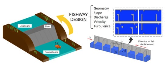
:Vertical slot fishways are increasingly common structures for the passage of a wide variety of migratory fish and contribute to the maintenance of fish diversity in fragmented rivers. These structures are designed with several geometric arrangements and, consequently, flow patterns through them can be shaped to present suitable characteristics for the fish species. To aid in the design of vertical slot fishways, a three-dimensional numerical model was used to simulate the flow for different geometric configurations. An existing vertical slot fishway with nonstandard dimensions was initially modeled and validated. This geometry was used as a reference design. Modifications to the reference design, such as the insertion of cylinders, changes in the baffle shape and position of the vertical slots, as possible rehabilitation measures, were proposed and tested. In summary, five different designs were evaluated with several slopes, totaling 17 geometries. Hydraulic parameters, flow patterns, maximum velocities, velocity fields and turbulence kinetic energy in the pools were analyzed. The results indicate that the maximum velocity values were between 9% and 68% higher than those obtained by the theoretical equation. This indicates that maximum velocities can be underestimated for nonstandard vertical slot fishways if a simplified evaluation is conducted. The insertion of cylinders in the region close to the slot reduces the maximum velocity up to 8.2%. The positioning of the vertical slots on alternating sides increases the maximum values of turbulence kinetic energy and the regions subjected to higher values. However, this configuration provided greater energy dissipation and reduction of velocities by up to 27%. Thus, modifications in nonstandard vertical slot fishways can be useful in future design or rehabilitation of existing structures in order to provide velocities and turbulence more friendly for a higher number of fish species.
1. Introduction
The river fragmentation caused by the construction of physical barriers prevents the movement of fishes among other environmental impacts. This effect may result in the disappearance of many species of ichthyofauna, mainly migratory, which move upstream during the reproduction phase [1,2].
To diminish this negative effect, fishways have been implemented for operation during the life of physical barriers. Fishways are structures or systems that allow for the movement of ichthyofauna between the downstream and upstream parts of a barrier, permitting the passage of migratory fish that move towards the headwaters of a river. Technical fishways include pool fishways, vertical slot fishways (VSFs), Denil fishways, eel ladders, fish locks and fish lifts [3].
An effective fishway should attract migratory fish quickly and allow them to enter, pass through the pools and leave safely with minimal costs in terms of time and energy. If the velocity and turbulence kinetic energy in the pools are very high, or if the water depth is too low, the fish will not be able to swim through the structure. Therefore, the biological efficiency of a fishway project is influenced by hydrodynamic variables such as velocity, water depth and turbulence fields in the pools [4]. To design an effective fishway, knowledge of swimming capabilities and hydraulic preferences of fish is required [5]. The goal of a fishway is not to be used by targeted species, but attracting a wide variety of fish species [6]. In South America, where there are approximately 4500 species [7], fishway design must focus on the species diversity of individuals.
The pool and VSFs consist in a channel with a succession of baffles that form pools. The flow through these fishways distributes the total head along the length of the structure [8]. They are designed to dissipate the energy of the flow to allow for the passage of fish without excessive effort [9].
VSFs have as a basic characteristic the transition between consecutive pools. This transition occurs through an opening along the entire depth of the pool (or nearly entire) that forms the vertical slot. Flows of VSF are considered favorable to many species of fish for three reasons: (1) in the transition region between consecutive pools, fish have the option to select the depth of passage, since the opening is across the depth; (2) in each pool, there is generally a large resting region where the velocities are much lower than in the main jet, which can be very favorable when a high number of pools are needed to overcome the vertical gradient [5]; (3) the main jet, where the maximum velocities are found, clearly identifies the upstream direction, which minimizes the chances of disorientation of fish along the route.
The geometric shapes that fall into this category of VSF are very diverse. There are many aspects that vary and influence the characteristics of the flow in a VSF, such as: the slope of the structure, distance between baffles (gap between consecutive pools), width/length ratio of pools, vertical slot width, shape and positioning of the smaller and larger baffles delimiting the vertical slot, relative positioning of vertical slots between consecutive pools, surface roughness of the channel and baffles, and the presence of additional elements along the structure (e.g., cylinders, and solids of various shapes inserted in the bottom). Rajaratnam et al. [10,11] conducted studies that considered wide variation of the geometric configurations of VSF, with 18 designs and slopes varying between 5% and 15%. After this work, a sequence of studies has focused mainly on the design optimization of VSF through analysis of flow velocities and turbulence patterns [12,13,14,15,16,17,18]. It has been verified that turbulent parameters can significantly influence fish behavior in the fishways as these can cause fatigue or confuse them in their passage through the hydraulic structure [19,20,21,22,23,24,25].
Experimental studies have been developed to investigate the flow in various geometries of fishways, mostly in scale models [10,11,16,22,26,27,28,29,30,31,32,33,34,35,36], and some evaluations that have used data obtained from real structures [15,17,37,38,39,40]. These experimental data are of great importance for understanding the flow, for establishing adequate criteria according to fish species and their swimming characteristics, and for adjusting numerical models of flow.
The use of computational fluid dynamics (CFD) to analyze hydraulic environments and environmental problems has emerged as a powerful and practical tool [41]. Over the last few years, different applications of numerical models have been developed to analyze flow in fishways. Many of these applications are based on the use of two-dimensional (2D) hydrodynamic models in the horizontal plane [4,42,43,44], for simulations of VSF, where the velocity field is essentially two-dimensional when the slopes are low, with a negligible vertical component of velocity in the whole basin, except in the region of the slot. These simplifications are not valid for other fishways, such as those with weirs and orifices, since the vertical component of velocity has significant values in the pools and cannot be overlooked. As well as in VSFs with high slopes [33], or for analysis of the flow in the region of the slot where the maximum velocities and vertical velocity components occur. In these latter situations, the flow is better evaluated with three-dimensional (3D) hydrodynamic models. Some uses of 3D CFD for evaluation of flow in fishways are presented in [45,46,47,48,49,50,51,52].
Successful fish passage is partially related to the understanding of how species interact with hydrodynamic flow conditions and the identification of flow characteristics that favor attraction and flow patterns that repel fish [5]. Fish swimming can be classified into sustained, prolonged and burst [53,54]. The sustained swimming is aerobic, characterized by a speed that can be maintained for at least 200 minutes without fatigue [55]. On the other hand, the burst swimming is anaerobic and it is the maximum speed that a fish can maintain for brief periods of less than 15 seconds [54], depending on the size of fish [53]. For many fish species, the capacity for burst swimming is important for their well-being and existence, mainly if the species ascend waterways in the spawning migration [53]. When designing fishways, the flow velocity should not be greater than the maximum that the fish can reach when crossing the structure.
Rajaratnam et al. [11] verified that VSFs with pools with a length of 10b0 and a width of 8b0, where b0 is the slot width, presented the more satisfactory performance. VSFs with this ratio of pool’s dimension (e.g., [26,33,56]) or close to this (e.g., [12,18,34,57]) are considered standard VSFs in this manuscript. However, it is usual to find VSFs built with other dimension ratios. For example, in Hydro Power Plant (HPP) Blanca, in Slovenia, 5.08b0 and 3.73b0 are, respectively, the length and the width of the pools of the VSF [40]; in Canada, the Vianney-Legendre VSF has pools with a length of 5.75b0 and a width of 4.9b0 [15]; in Brazil, the VSF of HPP Igarapava has pools with a length and a width of 7.5b0 [39]. The flow characteristics in nonstandard VSFs may be inadequate for fish use. In this work, we analyze the flow in nonstandard VSFs using 3D CFD resources. The studies are carried out on a full-scale model, reproducing a selection of nine pools from a VSF. We propose modifications in a reference geometry to make the flow less selective. The width and length of the pools, as well as the width of the slot, remain constant. The modifications are related to the insertion of cylinders in the pools, changes in baffle shape and position of the vertical slot. In addition, the sensitivity of flow behavior for several values of discharge and slope is assessed. This study aims to contribute to the design of new nonstandard VSF and to improve existing nonstandard VSFs by changes in geometry that result in better flow patterns.
2. Materials and Methods
2.1. Scope of the Research
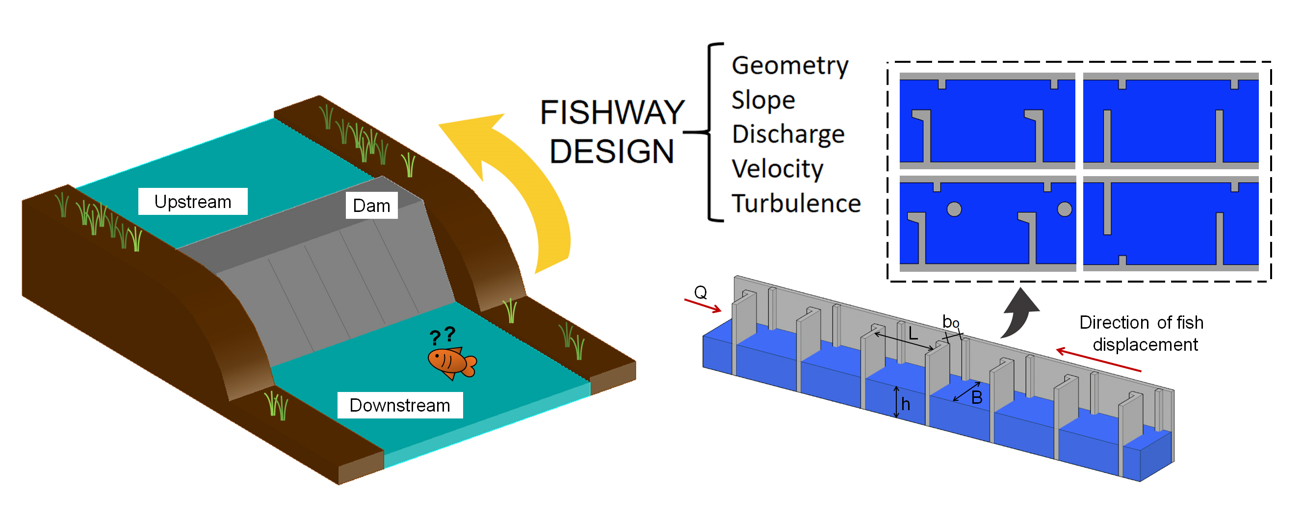
An existing VSF with nonstandard dimensions (HPP Blanca, [17]) was selected as the reference design for this study. This fishway has pools that are 3 m long, and 2.2 m wide, and have a vertical slot width (b0) of 0.59 m (length = 5.08b0 and width = 3.73b0) and a slope of 1.67%. Numerical flow simulations were conducted for nine consecutive pools of this reference design, plus an inlet and an outlet region, totaling 46 m in length (Figure 1, Figure 2a). The results obtained from the real structure [17], and previous numerical simulation [44] provided the initial parameters and boundary conditions of this work as the data to validate the numerical scheme. In order to evaluate discharge and slope influence in nonstandard VSFs, the reference design D1 was simulated for several discharges and slopes.
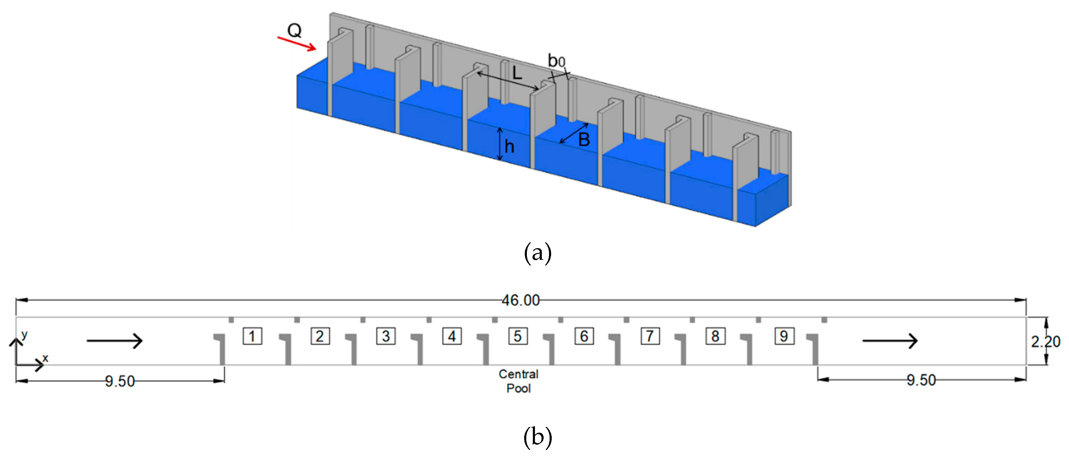
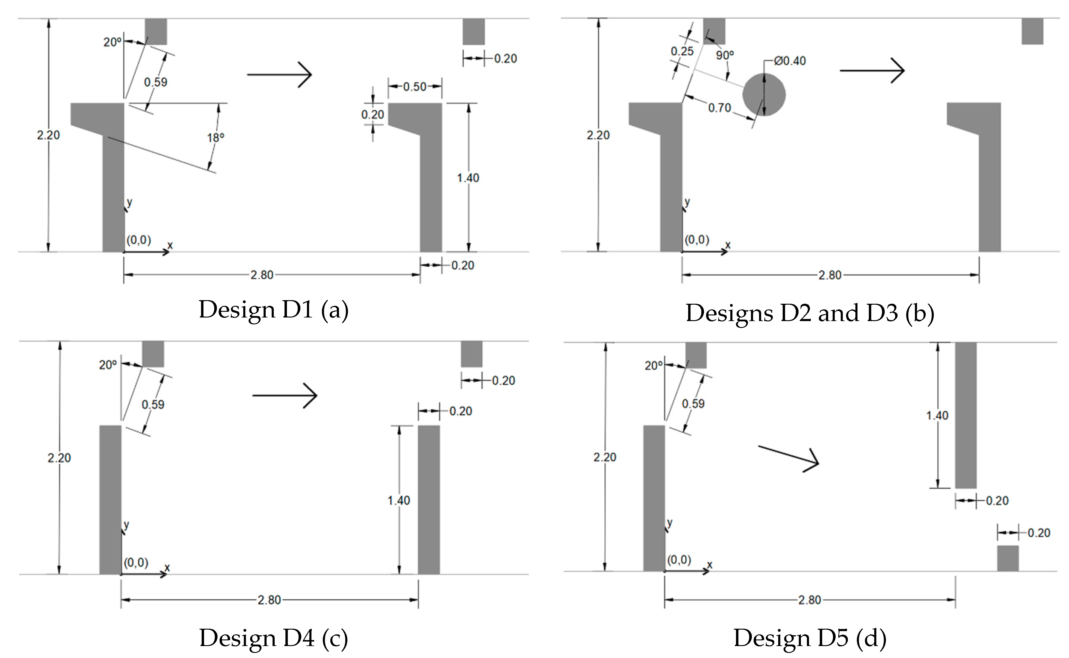
In the second step, several designs were proposed as modifications to the reference design to evaluate its impact on flow behavior. The modifications consisted in inserting or removing elements of the geometry. One of the changes consisted of inserting a cylindrical element positioned after the opening between the baffles (Figure 2b), as already proposed in previous studies [30,51,58,59]. Cylindrical elements (0.4 m in diameter) with heights of 0.4 m (design D2) and 0.2 m (design D3) were tested. It was decided to include cylinders with heights lower than the depth of the flow to maintain a free region in the upper part, facilitating the transit of larger individuals that support higher speeds. The VSF baffles are generally molded into an "L" shape. Two other designs with the larger "L"-shaped baffle replaced by a vertical wall of constant thickness were also tested. In these last configurations, the vertical slots were positioned all on the same side (design D4, Figure 2c) and on alternate sides (design D5, Figure 2d). The design D5 may be interesting from the point of view of energy dissipation and reduction of maximum velocities. In this way, it is expected that the maximum velocities would decrease, favoring fish with limitations related to flow velocity.
For simulations of the reference design, D1, we used the discharges 1.000 m³·s−1, 1.398 m³·s−1, 1.586 m³·s−1 and 1.765 m³·s−1, respectively, for the four slopes (1.67%, 3.33%, 5.00%, and 6.67%), which resulted in a mean depth of the pool flow as that in Bombač et al. [44], with a maximum variation of 2%. These slopes were also chosen considering the maximum velocities expected. In order to assess the influence of the discharge, four other values of discharge were tested for each slope. For the slope of 1.67%, the four additional discharge values are the same as those in Bombač et al. [44]. For other slopes, each one of the discharge values was defined in order to obtain a mean depth of the pool flow close to the found with the slope of 1.67%.
Simulations for the modified designs D2, D3 and D5 were carried out with four slopes (1.67%, 3.33%, 5.00%, and 6.67%). For design D4, only the slope equal to 1.67% was tested as the velocities obtained were already higher than the ones in the reference design.
For simulations of the modified designs, we used the discharges 1.000 m³·s−1, 1.398 m³·s−1, 1.586 m³·s−1 and 1.765 m³·s−1, respectively, for the four slopes (1.67%, 3.33%, 5.00%, and 6.67%). Discharges and conditions tested in all geometries are presented in Table 1, totaling 17 geometric configurations and 33 simulations (Table 2).
All the simulations were carried out using full-scale dimensions. All simulations were performed in steady state. In Supplementary Materials (Figure S1), the flow depth along the nine pools of the model is presented. There are differences between the first and the last pool, but the central pool can be considered in uniform or quasi-uniform conditions [60].
2.2. Governing Equations
The Ansys-CFX [61] was used for 3D numerical simulation of the flow. This program has been successfully used in other analyses of flow in VSFs, for example by Heimerl et al. [46] and Marriner et al. [15].
The model uses the finite volume method to solve the flow equations. Turbulence was modeled using the Reynolds decomposition, Reynolds Averaged Navier-Stokes (RANS) in 3D.
The equations of continuity and momentum solved by the program are, respectively:
where ρ is the fluid density; Vi represents the velocity time series, which can be divided into an average component and a time-varying component; μ is the molecular viscosity of fluid; is the turbulent viscosity of fluid; is the modified pressure and SM is the sum of the body forces [61]. The modified pressure is defined as:
where p is pressure and k is the turbulence kinetic energy.
The k-ε turbulence model [62] was used. The k-ε turbulence model has been widely tested and successfully applied to determine the turbulence viscosity for a large range of complex flows. The k-ε model is most commonly used to represent turbulence in fishway modeling [14,23,47,49,50,63,64,65,66].
In the k-ε model, the turbulent viscosity () is related to the turbulence kinetic energy (k) and turbulence dissipation rate (ε) and described as:
where is a dimensionless constant and equal to 0.09. The values of k and ε are taken directly from the differential transport equations. More details can be found in Ansys [61].
Some studies have used Large Eddy Simulation (LES) to evaluate the flow in fishways [35,49,51,67] and this model can provide more details about the flow than RANS [68]. However, the turbulence models based on RANS demand lower computational resources and they are much affordable, compared to LES [69] and can simulate adequately larger spatial scales corresponding to the time-averaged flow [68].
The free surface between air and water was modeled using the volume of fluid (VOF) method, where each computational cell is composed of fractions of each of the two phases (water and air). The VOF method solves the set of momentum equations in the domain, while storing the volume of the two phases in each computational cell.
2.3. Boundary Conditions and Discretization
Boundary conditions were applied to all faces of the domain. The non-slip boundary condition was applied to all walls (bottom, lateral walls, and baffles). The roughness of the walls was considered null in all situations. The consideration of null roughness is valid, since previous studies have pointed out that surface roughness does not play an important role for this type of flow [40,70].
At the inlet, the mass flows of water and atmospheric pressure to the part corresponding to the air were used. A high turbulence intensity (10%) was applied at the inlet to specify the turbulence kinetic energy and the energy dissipation rate of the flow. Previous studies demonstrated that the simulated velocities are graphically indistinguishable for turbulence intensities between 1% and 10% as also observed by Ma et al. [71] and Baki et al. [65].
At the outlet of the domain, the hydrostatic pressure distributions for the water fluid and atmospheric pressure for air were considered. An initial depth of the flow corresponding to the value obtained experimentally for the geometries D1, as presented in Bombač et al. [44], was used. For the other geometries, the same initial depths used in D1 were informed for the corresponding slopes. Initial depth sensitivity studies indicated that the depth results obtained in the simulations were not influenced by the initial conditions considered, as also reported by Baki et al. [65].
The top surface of air was defined as an open boundary [65] with atmospheric pressure [72] and zero gradient. The simulation considered the flow in an incompressible isothermal condition, maintaining constant physical properties of the water.
A preliminary analysis was performed to evaluate the mesh independence in the results. Three different meshes were tested for the same geometry and discharge. The three meshes tested were unstructured tetrahedral with refinement close to the walls and with mesh adaptation at the air–water interface. The number of elements in each mesh was 1.8 × 10⁶ (coarse mesh), 2.7 × 10⁶ (medium mesh), and 6.1 × 10⁶ (fine mesh), at the beginning of the simulation (the final number of elements is greater due to mesh adaptation). In Supplementary Materials (Figure S2), each mesh is presented. We also present velocities components obtained with the three meshes in Supplementary Materials (Figure S3). To check grid independence, we used the grid convergence index (GCI) [73,74]. The refinement ratio between the fine and medium meshes was 1.31, and that between the medium and coarse was 1.14. The GCI was calculated for velocities in 112 points in cross sections I, II, III and IV (Figure 3) in a plane parallel to the bottom (z/h = 0.4). The GCImedium/fine was 5.6% and the GCIcoarse/medium was 1.5%. Considering the GCI index and the comparison presented in Figure S3 (Supplementary Materials), we selected the medium mesh with at least 2.7 × 10⁶ elements in the beginning of the simulation. The meshes used in the simulations have an appropriate balance between accuracy and computational cost.
2.4. Data Analysis
Some hydraulic characteristics that can be useful to describe the flow in fishways were evaluated: the theoretical maximum velocity (Equation (5)), the discharge coefficient (Equation (6)), the Reynolds number (Equation (7)) and the Froude number (Equation (8)) in the slot, and the volumetric dissipated power (Equation (9)), which are written as:
where g is the gravitational acceleration, is the hydraulic drop per pool, Q is the volumetric discharge, b0 is the slot width, h is the mean depth of water in the pool, ρ is the water density, µ is the water molecular viscosity, B and L are the width and length of the pool, respectively, and h is the mean flow depth measured at the center of the pool.
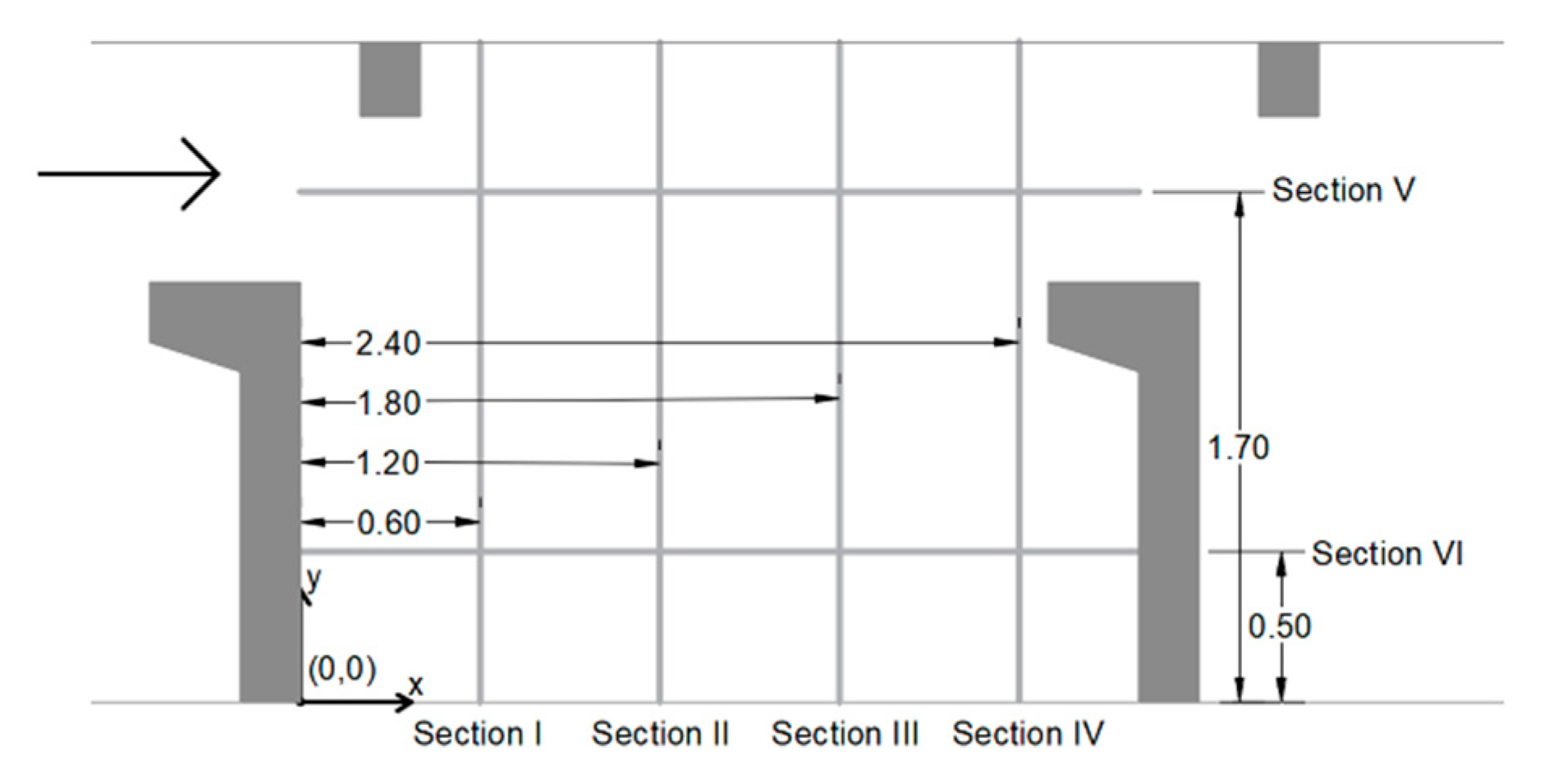
The results of the simulations are presented for the central pool in planes parallel to the bottom, and transverse and longitudinal to the axis of the fishway. The planes parallel to the bottom were positioned in three different z/h positions (0.2, 0.4, and 0.6), where z is the distance from the bottom to the plane, and h is the mean depth of the pool, measured in the middle of the central pool. Figure 3 shows the positioning of cross sections I, II, III and IV, which correspond to the planes at x = 0.60 m, x = 1.2 m, x = 1.80 m, and x = 2.40 m, respectively, and two vertical planes parallel to longitudinal axis of fishway (sections V and VI), which correspond to the planes at y = 1.70 m and y= 0.50 m, respectively. These sections were used to compare the results obtained in the simulations with the experimental results of Bombač et al. [17].
The results are presented for velocities magnitudes (V), and for velocities components: Vx (longitudinal), Vy (transversal), and Vz (normal to the bottom, z-component). The turbulence kinetic energy (k) was also evaluated.
The model validation is presented in Supplementary Materials (Figure S4).
3. Results and Discussion
3.1. Main Hydraulic Characteristics for All Designs
The main hydraulic characteristics obtained in the simulations—the mean flow depth (h), maximum velocity (Vmax) and the ratio of the experimental maximum value to the theoretical maximum value (Vmax/Vmaxt), discharge coefficient, Reynolds number and Froude number in the slot and the volumetric dissipated power—are presented in Table 2.
Analysis of the basic hydraulic characteristics of the flow in the different geometries tested shows that the resulting velocity obtained for each simulation was between 9% (D5S4) and 68% (D1S1, and D1S2) higher than the theoretical maximum value.
Generally, fishways constructed in South America use reference speeds of 2 m·s−1 based on proposed criteria for salmonids and fish present in the Northern Hemisphere. For most species of neotropical migratory fish, there is no data on swimming capacity in terms of the endurance and speed [7]. However, some studies have been conducted over the past two decades. Santos et al. [7] evaluated the prolonged critical speed and burst speed of the piau (Leporinus reinhardti) and found, for example, a sustained critical speed of 1.28 m·s−1 for an individual with a length of 15 cm and a burst speed of 1.72 m·s−1 were maintained for 20 seconds for a fish being 16 cm in length. In later studies, the same authors evaluated the behavior of the mandi-amarelo (Pimelodus maculatus) and found, for example, that for an individual being 15 cm in length, the critical prolonged velocity is 1.10 m·s−1, which is less than that of the piau [2].
Considering the comparison between the maximum velocity results from the present study and those obtained in previous analyses, some questions regarding the flows in fishways are relevant: Can the theoretical maximum velocity be used as the maximum reference velocity? If the observed velocities are considerably higher than those theoretically obtained, what are the maximum values that should be adopted? There are studies [15,34,50], among others, found that when comparing the theoretical maximum velocity with the measured and/or simulated maximum values, the latter were less or very close. Other studies have found results similar to these obtained in the present study, with measured/simulated velocities in VSFs higher than those theoretically obtained [17,30,44,75], for example. As one of the geometries analyzed in this study, D1S1 is the same as that investigated by Bombač et al. [44], where there are experimental and simulation data, and velocities up to 60% higher than the theoretical values have been observed; the results of the present study can be considered consistent and it is reasonable to conclude that the theoretical maximum velocities may underestimate the maximum velocities of the flow. This fact has important consequences for the design of these structures, since the underestimated flow velocity represents a possible barrier to the displacement of some species of fish.
One characteristic of the geometries analyzed in this study, which may be responsible for higher than expected velocities by the simplified theoretical equation, is related to the ratio of pool dimensions to slot opening. Most VSF geometries use pools with length and width dimensions of 10 and 8 times the slot width, respectively, following recommendations in Rajaratnam et al. [10,11]. In this paper, we evaluate nonstandard VSF geometries with a length and a width of 5.08 and 3.73 times the slot width, respectively. Thus, the size of the aperture in our geometries is much higher than in the most frequently used geometries, which makes the maximum velocity higher. One can imagine a limiting situation in which the gap between baffles is close to the width of the channel, and where the vertical baffles nearly disappear. In this situation, the flow will be practically equal to the flow in one channel, without the dissipation of energy inside the pool, as is typically expected in VSFs. This brings into question the reason for analysis of designs with geometric relationships distant from what is generally considered more adequate. It should be noted that the aperture between baffles is a characteristic that must be defined considering the dimensions of the target fish. The pool should be defined by the relation proposed by Rajaratnam et al. [10,11]. In this case, maintaining an opening width of 0.59 m would lead to a geometry with very large pools measuring 6.00 m long and 4.70 m wide, which is uncommon and could encouraged the use of nonstandard VSFs.
The discharge coefficients ranged from 0.82 to 1.40, with most of the values greater than unity. For each design, an increase in slope resulted in the reduction of the discharge coefficient. The values found are slightly higher than those generally attributed to these structures (0.30 to 1.30), as presented in Rajaratnam et al. [10,11] for a wide variety of geometries, different in dimensions and slopes than the ones we have tested. This fact is consistent with the maximum velocities found, which were higher than the theoretical maximum values.
The Reynolds number in the slot for all geometries varied between 6 × 10⁵ and 1.4 × 10⁶. It was observed that higher values are associated with higher slopes and that the insertion of cylindrical elements or the alternation of the position of the vertical slot in the pools reduces the maximum velocities of the flow and consequently the Reynolds number. According to Wu [76], the Reynolds number lies in the range of 104 < Re < 108 for several fish species swimming normally. The Froude number is always less than unity, characterizing subcritical flow in all the simulations performed, with the highest values associated with the configurations with the highest slopes.
For the geometries analyzed in this study, the volumetric dissipated power (PV) varied between 52 and 445 W/m³. PV is a simple parameter and possibly the first criterion proposed to compare the adequacy of the flow in pools to the possibility of use by the fish. Many studies have used this parameter as an indicator of the flow turbulence in pools, associating ranges of PV to certain species of fish. Bell [77] presented the limit of this parameter as equal to 191 W/m³, considering that this value represents the maximum energy dissipation inside the pool tolerated by fishes. Subsequently, other limits were proposed; for example, for salmonids the upper limit of 200 W/m³ [3,8], or 250 W/m³ [57] is generally used, while for cyprinids fish around 150 W/m³ is used [3,8], with some variation of these values according to the reference in question. Considering the values found in this study and the limits presented in the literature, some of these geometries, especially those with greater slopes, are not suitable for use by most species of fish. However, it has been observed that many structures with similar Pv values have different mean and turbulence flow patterns, which draws attention to the observation of this parameter and the maximum velocity which can be used in the first analysis [34], but may be insufficient to assess the adequacy of the flow to the fish traffic [57]. The evaluation of flow velocities time series, obtained experimentally or through numerical simulation, allow for the evaluation of turbulence parameters, such as turbulence intensity, Reynolds shear stress and turbulence kinetic energy. These parameters provide information useful to establish relations between turbulence patterns and fish behavior [21,31,57,78,79,80].
3.2. Effect of the Slope and Discharge in the Reference Design D1
The velocities in different planes parallel to the bottom (z/h = 0.2, 0.4, and 0.6) are shown in Figure 4. It can be observed in the various planes that the higher velocities are in a way connecting consecutive pools, forming a main jet. The extreme values of velocities occur close to the inlet of the pool in the main jet region, indicating that there is dissipation of the energy of the flow inside the pool, with reduction of velocities in the jet as it moves downstream. In addition, adjacent to the main jet, there are regions with much smaller velocities [10,11,16,27,33,34,57]. Among the larger baffles, there is a large region with lower velocities than the main jet, which can be used as a resting zone by the fish during the transit process in the structure. Comparing the corresponding planes of different slopes, we can see that the main variation between velocity fields occurs in the region of the main jet, which presents higher velocities for the geometries of higher slopes [26,34,44]. A four-fold increase in the slope (from 1.67% to 6.67%), maintaining the mean flow depth in the pools, requires a discharge increase of 76.5% and results in an increase of maximum velocities (V) up to 80%. These results reinforce the importance of the role of the bottom slope in the flow. For the slope of 1.67%, the maximum velocity exceeded 1.5 m·s−1 in only some regions of the pools. For the higher slope tested, the maximum velocity exceeded 2.5 m·s−1 in about 8% of the pool. The results show the most important parameter in the determination of the discharge and the maximum velocities in VSFs is the hydraulic drop per pool, which is directly related to the slope of the structure, along with the slot width [44]. When comparing velocity fields for the same discharge and slope, positioned at different distances from the bottom, it can be observed that there are higher velocities in the main jet for the planes nearer the bottom and, for the greater slopes, the differences are more pronounced. In the recirculation zones, the flow pattern is similar in different planes parallel to the bottom for the same discharge and slope. This information indicates that the flow, while presenting a well-defined pattern of main jet and recirculation zones between larger baffles, also has the z-component of velocities in the region of the main jet.
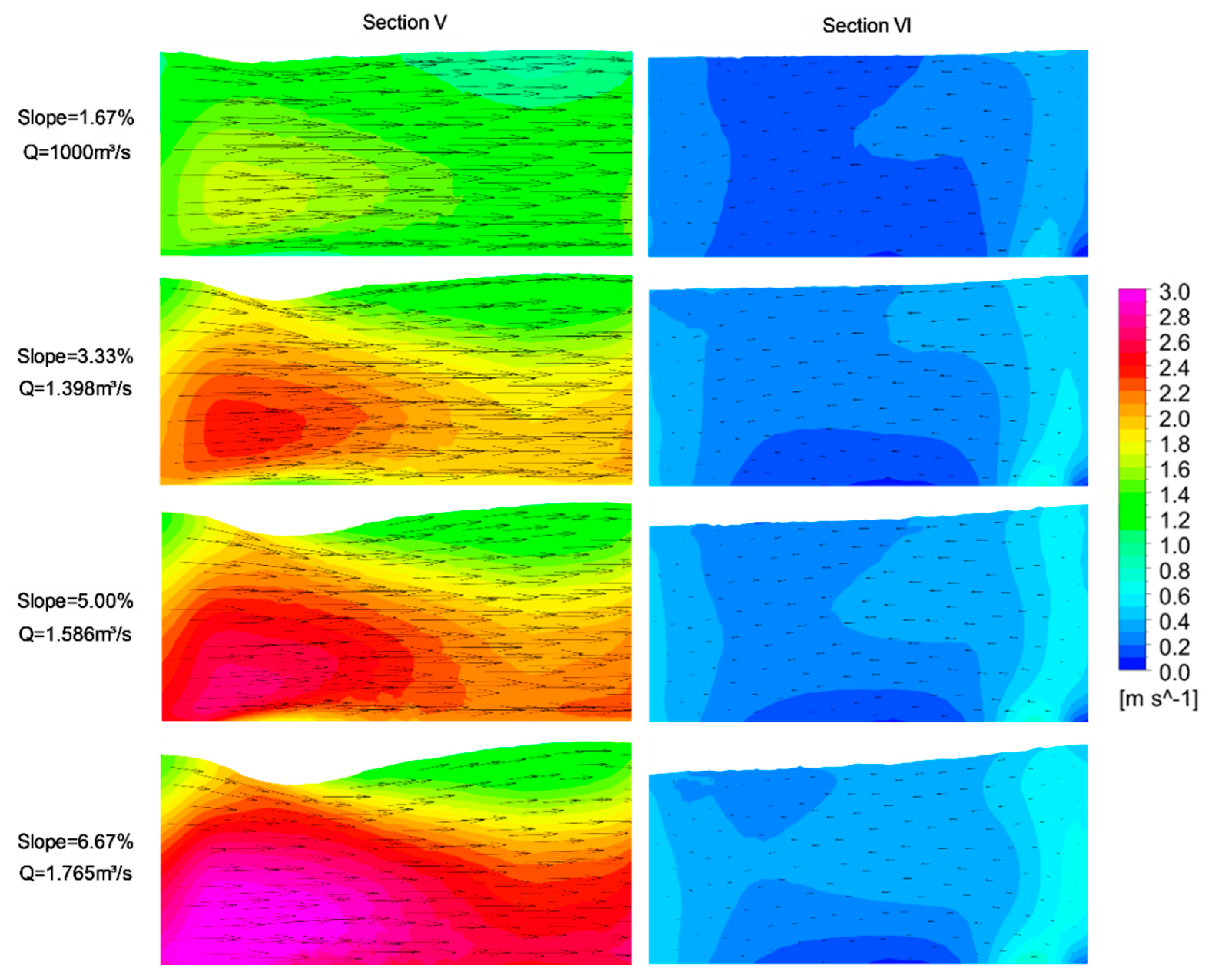
Figure 5 shows the behavior of velocities in vertical planes parallel to the longitudinal axis of fishway. In section VI (y = 0.5 m, Figure 3), which passes through the region between the larger baffles, it can be observed that the velocities are lower in the central part, inferior to 0.5 m·s−1, characterizing the resting zone inside the pool. At the extremities, which are the regions closest to the baffles, the velocities are slightly higher (close to 1.0 m·s−1), indicating the outermost region of the recirculation, as seen in the planes parallel to the bottom (Figure 4). In section V (y = 1.7 m), which is a plane passing through the main jet, the presence of velocities much higher than those present in section VI is quite evident, with the maximum occurring at the beginning of the plane, in the jet entrance of the pool. In the plane that passes through the main jet, it can be seen that there is a strong influence of the bottom slope, with higher velocities as the slope increases. As far as the velocity distribution along the vertical profile is concerned, for the plane passing through the resting zone, there are no important vertical variations and neither are expressive vertical velocity components. For the plane that passes through the main jet, there are important vertical velocity components, mainly in the region near the entrance of the flow in the pool. In the positions located from the bottom to the half depth, we can see a concentration of maximum velocities, with few vertical components. In the more superficial layers of the flow, it is noticed that there are components of vertical velocities descending in the region of the entrance of the jet in the pool, with z-components of velocity of up to −0.75 m·s−1 (39% of the velocity in the plane parallel to the bottom) for the higher slope tested. Vertical velocities of 20% of the maximum velocity at the slot were found in standard VSFs [26] with a slope of 10.52%. As the flow runs longitudinally inside the pool, z-components of velocity are again less expressive, ranging between −0.2 m·s−1 and 0.2 m·s−1 (between −0.3 m·s−1 and 0.3 m·s−1) in more than 99% (97%) of the pool for the slope of 1.67% (6.67%). The vertical velocity in the majority of the regions of the pool is less than 5% of the velocity in the plane parallel to the bottom, as reported by An et al. [50]. The vertical velocity less than 3% of the maximum velocity in the slot was reported [26] in most areas of the pool for a standard VSF (Design 18, [11]). At the end of the pool upstream of the long baffle, the maximum upwelling velocities are located, as reported by [26]. The differences between the velocities in the surface and in the bottom are below 10% in the areas out of the main jet in the pool.
These results indicate that the representation of the 3D flow is more important for the region near the vertical slot [58] and for the higher slopes, as observed by Wu et al. [33] and Liu et al. [26], for example. This result reinforces that the 3D flow simulations are useful and necessary tools for better evaluations of the flow in VSFs [52], mainly in the region near the slot, which is precisely the critical area for fish traffic. Studies have shown that the components of ascensional/descendancy velocities have important impacts on the behavior of fish, and this should not be neglected [20,81]. The simplest, 2D models allow for the analysis of the flow in the rest of the regions of the pools, where the flow predominantly presents velocities with components in a plane parallel to the bottom.
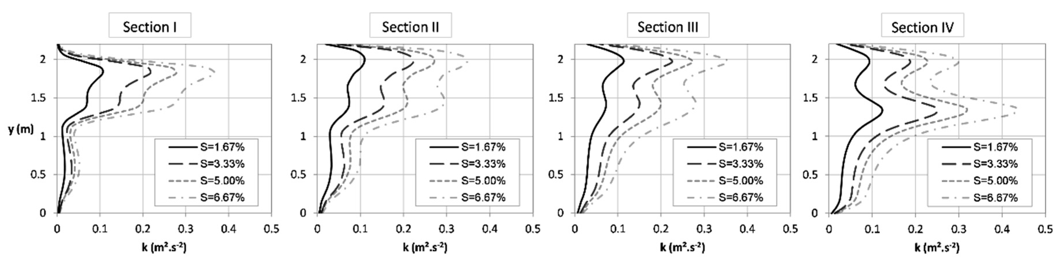
Figure 6 compares the turbulence kinetic energy, k, for the four slopes tested in the four cross sections (i.e., I, II, III and IV) in the plane where z/h = 0.4. Analyzing the effect of slope on the turbulence kinetic energy behavior, it can be verified that the highest values were obtained for the highest slopes in each section of analysis. A four-fold increase in the slope (from 1.67% to 6.67%), maintaining the mean flow depth in the pools, results in an increase of turbulence kinetic energy (k) up to 250%. It is important that limits and preferences of turbulence kinetic energy should be considered in the design of fishways. Studies in a pool-type fishway with Iberian barbel (Luciobarbus bocagei) showed that small and large adults used mainly areas with k < 0.05 m²·s−2 [21]. In a VSF, silver carp (Hypophthalmichthys molitrix) spent more time in the range of turbulence kinetic energy of 0.02 to 0.035 m²·s−2 [82]. The single analysis of the four cross sections shows for all situations values of k < 0.43 m²·s−2. Two regions of maximum values of k in each section were observed. They are between the transition between the main jet and the recirculation zones. As the flow approaches the larger baffle downstream, it is more pronounced. This indicates that the maximum values of k do not coincide with the maximum velocities. Further analyses for the all pool are shown in Section 3.3, comparing all the geometries evaluated.
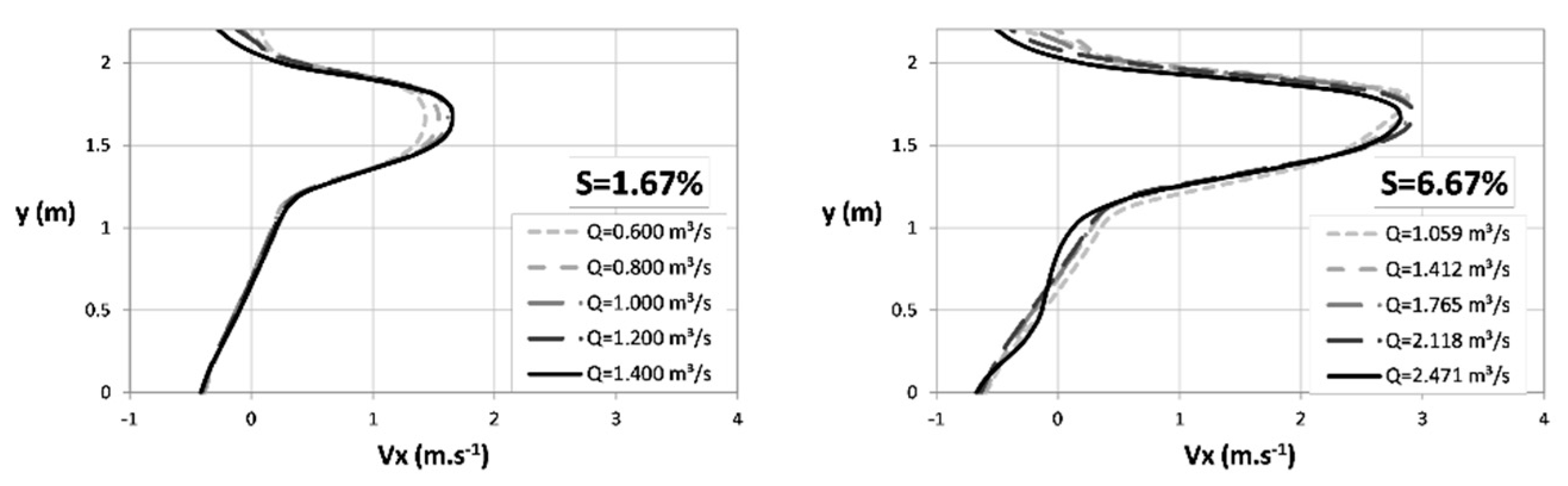
Figure 7 shows the longitudinal velocities, Vx, in section I, with different slopes and discharges. For the same slope, the variation of the discharge is reflected in variation of the depth of the flow in the pool (Table 2), and has little influence in the variation of the velocities [58]. The same slope with flow variations of more than 100% resulted in velocity variations of up to 15%. The highest velocity variations occur for the geometry with the smallest slope and the lowest variations for the highest slopes tested, with the maximum values not necessarily associated with higher discharges. These results show that for one slope, velocity patterns in the pools depend strongly on the position of each point itself, it is independent of the discharge [29,34,52,58] and it is weakly influenced by the vertical position (except for the jet region) [58]. This is a very favorable feature for the use of VSF, differentiating it from other fishway models, such as those with superficial weir, for example. Thus, fish will not encounter additional displacement problems inside a structure in steady flow with a wide range of discharges, as long as a minimum depth of flow, associated with the dimensions of the target fish, and a uniform flow are maintained.
3.3. Effect of Modifications in the Reference Design
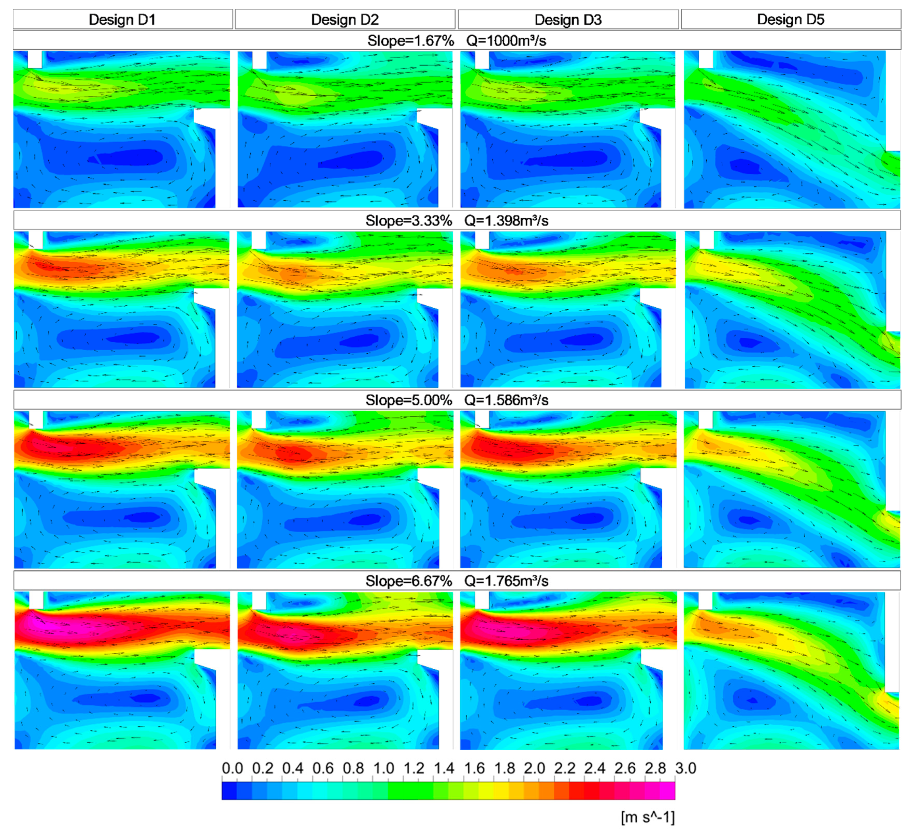
In Figure 8, the velocity distributions in planes distant from the bottom at z/h = 0.4 are compared between the reference design (D1), with the cylinder designs (D2 with a cylinder of h = 0.4 m and D3 with h = 0.2 m) and the design with slots positioned on alternate sides (D5) for the four slopes tested.
The analysis of the flow in the VSF with the cylinder positioned after the slot identified that a main jet between consecutive openings is maintained and that the maximum velocities are linked to higher slopes, as observed in the geometries without the presence of the cylinder. The comparison between the design with cylinder and the reference indicates that the presence of a cylinder can reduce the maximum velocities for the smallest and highest slopes between 1.3% and 8.2%, respectively, considering the cylinder height of 0.4 m, and those between 3.2% and 6.1%, considering the cylinder height of 0.2 m. In the comparison between the two designs with cylinders, it can be observed that the taller cylinder influences the behavior of velocities in a greater depth of flow and has a greater effect on velocity reduction than the shorter cylinder.
The alternation of the position of the vertical slot (design D5) causes a reduction of the maximum velocities and a reduction of the region of large recirculation (Figure 8). The reduction of the maximum velocity varied between 16% and 27%, with the highest values associated with the highest slopes. In design D5, a reduction of the resting region between the larger baffles was clearly observed, and an analysis of the behavior of the turbulence kinetic energy was carried out as presented below. The simplification of the geometry of the larger baffle maintaining the slots in the same position along the fishway (design D4) causes an increase of the maximum velocities (Table 2) in comparison with the reference design (D1) under the same discharge and slope. The maximum velocities are slightly higher for design D4, with values up to 7% higher for the region closest to the entrance of the jet in the pool.
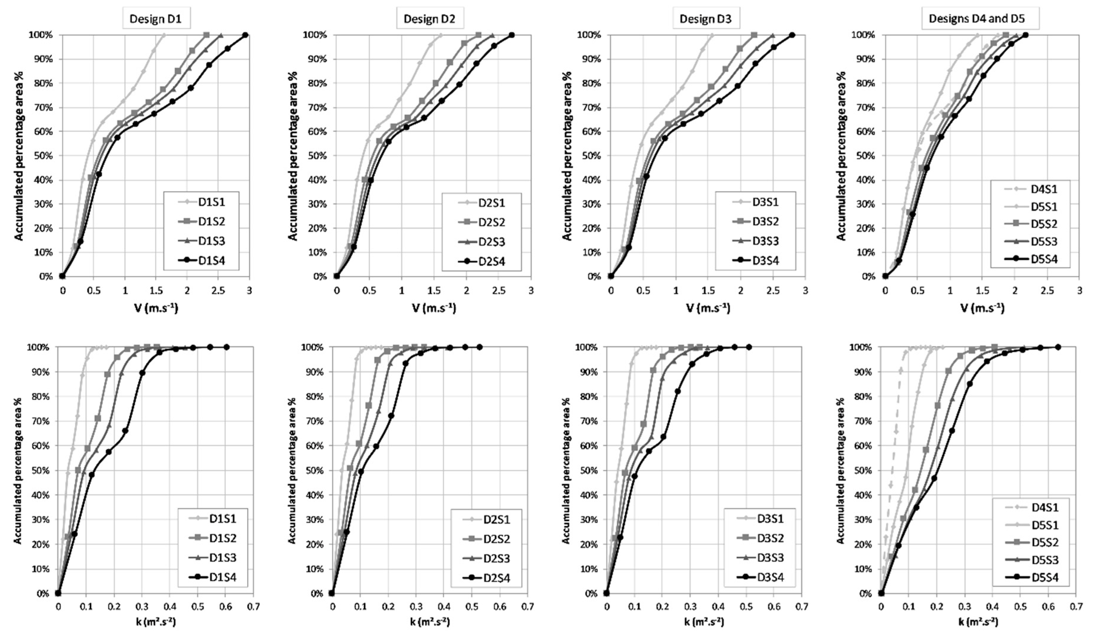
In addition, the velocity and turbulence kinetic energy fields of the five designs with different slopes and discharges were compared, considering their distribution in the pools. For the central pools of the geometries tested and for the z/h = 0.4 plane, the cumulative frequency distributions of velocities and turbulence kinetic energy are presented in Figure 9.
In the geometries with the slope of 1.67%, there is no significant variation in behavior between designs D1, D2, D3, and D4 by analyzing the velocity frequency distributions. For example, in designs D1 to D4, between 72% and 75% of the pool area has velocities below 1.0 m·s−1, whereas for design D5, velocities are lower and 85% of the pool area has velocities less than 1.0 m·s−1. For the higher slopes, the effect of geometry on the distributions of velocities in the pools area is more relevant. For a slope of 3.33% in design D1, 10% of the pool area has velocities greater than 2.0 m·s−1, and in approximately 25% of the pool the velocity exceeds 1.5 m·s−1, whereas for geometries D2 and D3, velocities greater than 2.0 m·s−1 do not exceed 6% of the pool area, and for geometry D5 this velocity is not verified in any region. For the highest slope tested (6.67%), the frequency distributions of velocities in the pools allow for verification that the reference design, D1, presents 24% of the pool area with velocities greater that 2.0 m·s−1, whereas for geometries D2, D3, and D5, the values are 18%, 20% and 5%, respectively.
The zones with velocities lower than 0.5 m·s−1 are smaller in the designs with higher slopes. For design D1, velocities are lower than 0.5 m·s−1 in 57%, 43%, 40%, and 34% of the pool area, for the slopes of 1.67%, 3.33%, 5.00%, and 6.67%, respectively. For designs D2 and D3, with the cylinders, in the plane at z/h = 0.4, these values are similar to the reference design. When it is evaluated in a plane that passes through the cylinder (e.g., z = 0.15 m), the zones with velocities lower than 0.5 m·s−1 decrease to 52%, 38%, 35% and 30% for the respective slopes in design D2. The decrease in the resting zones in the presence of the cylinders is in agreement with previous studies [58]. As large recirculation zones can be traps for small fish [58], its reduction by the insertion of the cylinder in designs D2 and D3 turns the fishway less selective.
The increase in the slope, for designs D1, D2, D3, and D5, resulted in an increase in the amplitude of the z-component of velocity (Vz). Comparing the amplitude of Vz for the design D1 with slopes of 6.67% and 1.67%, for example, in the former the values are 80% higher in the deepest layers and 115% higher for the surface layers of the pool. In design D2, the amplitudes of Vz are about 83% higher in the slope of 6.67% in comparison with the slope 1.67%, regardless of the layer position. Comparing designs D1 and D2, for the same slope, the insertion of the cylinder reduces the amplitude of Vz by 15% in the layers under the influence of the cylinder. It was observed the z-component velocities are less expressive in the major part of the pool, as it was verified for the reference design (Section 3.2). For example, in the deepest layers of design D2, Vz lies in the range between −0.3 m·s−1 and 0.3 m·s−1 in more than 97% (83%) of the area for the slope of 1.67% (6.67%). For the surface planes, there are more than 99% (94%) of the area for the slope of 1.67% (6.67%) with Vz ranging between −0.3 m·s−1 and 0.3 m·s−1.
For all the designs tested, the increase in the slope is responsible for the increase in downward velocity close to the slot entrance and increase in the upwelling velocity at the end of the pool upstream of the long baffle. Previous studies [30] have also verified that the presence of a cylinder reduced the vertical velocity. Considering that vertical velocities have demonstrated to influence the behavior of the fish [20,81,83], the insertion of the cylinder can benefits fish.
The analysis of turbulence kinetic energy frequency distributions for the slope of 1.67% shows designs D1, D2, and D3 having similar patterns. For example, for designs D1, D2, and D3, 58%, 59% and 56% of the pool area, respectively, have turbulence kinetic energy below 0.05 m2·s−2, which were the values associated with the preferred areas in studies with Iberian barbel (Luciobarbus bocagei) [21]. The maximum values of turbulence kinetic energy in designs D1, D2, and D3 are the same (0.17 m2·s−2). Thus, the insertion of the cylinders for the lower slope was not significant to reduce maximum velocities or turbulence kinetic energy. For the same slope of 1.67%, in designs D4 and D5, 62% and 30% of the pool area, respectively, have k < 0.05 m2·s−2. For design D4, the maximum turbulence kinetic energy was similar to the one obtained in the reference design. The design with the slots in alternate sides (D5) and the slope of 1.67% shows higher turbulence kinetic energy than the reference of up to 57%, and the maximum value of 0.22 m2·s−2.
In addition, for the slope of 6.67%, designs D1, D2, D3, and D5 present 20%, 23%, 22% and 15% of the pool area, respectively, with k < 0.05 m2·s−2. The maximum values of turbulence kinetic energy were reduced in the designs with the cylinders. The insertion of the taller (lower) cylinder in design D2 (D3) was able to reduce the maximum value of turbulence kinetic energy in 15% (12%), when being compared with the reference D1, of which the value is 0.60 m2·s−2. In design D5, the maximum turbulence kinetic energy was 7% higher than the observed one in the reference.
Data of turbulence kinetic energy, obtained in other VSFs (length = 14.18b0, width = 7.66b0, and b0 = 0.13 m) with a slope of 8.50% [67], reached up maximum values of 0.35 m2·s−2 and k < 0.05 m2·s−2 in 59% to 73% of the pool area. The present study obtained the higher maximum values and minor zones of the pool with k < 0.05 m2·s−2. Even with differences in the size of the pool and in the slope, it is probable that the nonstandard dimensions of the VSF in the present study are partially responsible for higher turbulence.
The maximum values of normalized turbulent kinetic energy (k0.5/Vmax) for designs D1, D2, D3, and D4 for the several slopes are between 0.24 and 0.26 and for design D5 between 0.33 and 0.36. The maximum normalized turbulent kinetic energy values for standard VSFs (Design 18, [11]) for slopes of 5.06% and 10.52% were 0.28 and 0.24, respectively [26]. The values of k0.5/Vmax are not efficient to characterize the turbulence in nonstandard VSF flow since both k and Vmax values are higher to those found in standard VSFs, resulting in similar values for different patterns.
The analyses from the ecological point of view are complex, mainly because there is a lack in understanding and quantification of the behavior of freshwater fish species [5]. If biological information is absent, the selection of fishway designs will consider the fish behavior observed in similar structures or the swimming capabilities and hydraulic preferences of other species. This is a trial and error approach that probably requires years to attain success [5].
The insertion of a single cylinder causes the reduction in velocity magnitude, in the z-components of velocity and in the turbulence kinetic energy, which are all positive points for the displacement of the fish [30]. It is a necessary further study to evaluate the fish behavior related with the vortex dynamics in the cylinder wake. Eddies of a similar diameter to the fish length associated with higher vorticity provide stability challenges to swimming fish [20]. Previous studies [30,58], with insertion of a single cylinder in the VSF, verified that this modification could allow for the correlation of VSF flow features to the swimming capabilities of small fish.
The flow in design D5 presented lower maximum velocities, but higher turbulence in terms of absolute values and distribution, in relation with the reference design. Silva et al. [31] evaluated pool-type fishways with orifices in a straight configuration and with orifices in alternating sides. The alternating sides orifices configuration presented most favorable hydraulic conditions than the straight one and it was the most efficient for passage of fish with different sizes. Experimental studies with fish in nonstandard VSFs with slots in alternating sides are required to verify if the reduction in the maximum velocities are still interesting if it is accompanied by higher turbulence.
Considering that fishways may be composed of many pools that connect the downstream and upstream sides of the physical barrier, a slight reduction of the flow velocities or in the turbulence kinetic energy in each pool can represent a great economy in the amount of energy that the fish spend along the total way. Results of velocities and turbulence kinetic energy show that the insertion of a cylinder (designs D2 and D3) can be a better measure in order to turn the flow in an existing VSF less selective. Tarrade et al. [58] verified that the passage through slots by the small fish became easier with the insertion of a cylinder close to the slot. Biological preferences of the fish present in one region will provide information to choose an appropriate design or rehabilitation measure.
If the velocities in the slot, which is a mandatory region for the passage in the VSF, are higher than the burst swimming speed, the flow in the fishway will represent an insurmountable hydraulic barrier. Thus, the flows on the nonstandard VSF for all designs we have evaluated with the slopes of 5.00% and 6.67% are incompatible to swimming capabilities of a wide variety of fish. Even the modifications we have tested in the reference design were not able to rehabilitate the nonstandard VSF for higher slopes. It is also clear that the design of new nonstandard VSFs associated with higher slopes must be avoided, unless specific studies shows the agreement between hydraulic characteristics and swimming capabilities.
4. Conclusions
Several geometries of nonstandard VSF were evaluated using a numerical 3D model. An investigation of the effect of the slope of the structure indicated that by increasing the slope four times (1.67% to 6.67%), the discharge is increased by 76.5% to maintain the same mean depth of flow in the pools and the maximum velocity is increased by 78.6%. The differences in the maximum velocities obtained in this study and those obtained by a simplified equation are also remarkable. For a pool with dimensions of a length and a width of 5.08 and 3.73 times the width of the slot, respectively, the velocities can be up to 68% higher than the theoretical prediction. Comparing data on the swimming capacity of neotropical fishes (e.g., [2,7]) with velocities found in the reference design indicates that the use in neotropical environments would be limited to structures with smaller slopes, so that velocities are compatible with the species present in these areas. Thus, it is quite useful to investigate interventions in the geometry of the structures, so that the flow is more fish-friendly in terms of maximum velocities and turbulent flow patterns. Modifications in the reference design were tested to obtain a less selective flow. The insertion of a cylinder after the passage of the flow through the slot allowed for the reduction of maximum velocities by up to 8% for the taller cylinder and up to 6% for the shorter cylinder, with greater influence for design with higher slopes. These analyses emphasize that the presence of a cylindrical element within the pool is beneficial in the sense of reducing the maximum velocities and reducing the areas subjected to higher velocities, which may be considered as hydraulic barriers to the movement of fish. The cylindrical element of greater height produces more significant and more extensive changes inside the pool. Simplified baffles resulted in maximum velocities up to 7% higher than those obtained in the original configuration. Considering that the reference configuration already exhibits values of maximum velocities that are limiting for several neotropical fish species, this modification was not considered to be a viable alternative, unless working with very low slopes where maximum velocities are still within the range of use. The positioning of vertical slots on alternating sides of the same pool clearly represents the most efficient tested alternative in the sense of reducing the maximum velocities and the areas subjected to them. This alternative proved to be quite efficient in reducing maximum flow velocities, reaching a reduction of up to 27% compared to the reference geometry. On the other hand, this configuration causes the recirculation region inside the pools, used for rest by the fish, to be reduced. Further, an increase in parameters indicative of the turbulence was observed, and the turbulence kinetic energy increased up to 57%.
The results from this study could be useful in the design of new nonstandard VSF as well as changes to existing nonstandard VSFs with the aim of obtaining a less selective flow. The results could also be used as input data for the estimation of fish habitat suitability indices for different system configurations, allowing for optimization of the design of these structures for the types of fish in the region, as proposed by Alvarez-Vázquez et al. [42,84] and Maeda [24]. The use of CFD allows for the estimation of the main variables of the fishway flow for different hydraulic conditions and diverse nonstandard geometries. This information can be considered in comparison with the ideal values required by different types of fish to be able to pass through the structure in the shortest time and consume the least amount of energy.
Supplementary Materials
The following are available online at https://www.mdpi.com/2073-4441/11/2/199/s1, Figure S1: Flow depth along the model: (a) dimensionless flow depth along the nine pools of the model; (b) line where the flow depth were evaluated—pools 1 to 9, Figure S2: Details in one pool of the three meshes tested: (a) coarse mesh (1.8 × 10⁶ elements); (b) medium mesh (2.7 × 10⁶ elements) and (c) fine mesh (6.1 × 10⁶ elements). The medium mesh was selected for the simulations, Figure S3: Longitudinal velocity Vx (m·s−1), transversal velocity Vy (m·s−1) and z-component of velocity Vz (m·s−1), at four cross sections I, II, III and IV (according to Figure 3), in the plane at z/h = 0.4 from the bottom, for a discharge of 0.800 m³·s−1, design D1S1 obtained through three meshes: coarse, medium and fine, S4. Model validation.
Author Contributions
All authors listed have contributed substantially to the manuscript to be included as authors. Conceptualization, D.G.S. and J.M.B.; data curation, D.G.S., J.B.R. and J.M.B.; formal analysis, D.G.S., J.B.R. and J.M.B.; investigation, D.G.S. and J.B.R.; methodology, D.G.S., J.B.R. and J.M.B.; project administration, D.G.S.; validation, D.G.S. and J.B.R.; writing of the original draft, D.G.S. and J.B.R.; writing of review and editing, D.G.S., J.B.R. and J.M.B. All authors read and approved the final version of the manuscript.
Funding
This research was funded by Conselho Nacional de Desenvolvimento Científico e Tecnológico of Brazil (444180/2014-1). J.B.R. received a scholarship grant from Universidade Federal do Rio Grande do Sul, Brazil.
Conflicts of Interest
The authors declare no conflicts of interest.
Symbols and Abbreviations
b0 = slot width [m]
B = width of the pool [m]
CQ = discharge coefficient [-]
Cμ = k − ε turbulence model constant [-]
Fr = Froude number [-]
g = gravity acceleration [m·s−2]
h = water depth [m]
k = turbulence kinetic energy per unit mass [m2·s−2]
L = length of the pool [m]
p = pressure [kg·m−1·s−2]
p′ = modified pressure [kg·m−1·s−2]
PV = volumetric dissipated power [W·m−3]
Q = volumetric discharge [m3·s−1]
Re = Reynolds number [-]
S = longitudinal slope [-]
SM = momentum source [kg·m−2·s−2]
t = time [s]
V = velocity magnitude [m·s−1]
Vmax = Maximum velocity [m·s−1]
Vmax t = Maximum theorical velocity [m·s−1]
Vx = mean longitudinal velocity component [m·s−1]
Vy = mean transverse velocity component [m·s−1]
Vz = mean z-component of velocity [m·s−1]
x = longitudinal coordinate [m]
y = transverse coordinate [m]
z = z coordinate, normal to the channel bottom [m]
ε = turbulence dissipation rate [m2·s−3]
∆h = hydraulic drop between two adjacent pools [m]
μ = molecular viscosity [kg·m−1·s−1]
μt = turbulence viscosity [kg·m−1·s−1]
ρ = density [kg·m−3]
CFD = computational fluid dynamics
GCI = grid convergence index
HPP = Hydro Power Plant
LES = Large Eddy Simulation
RANS = Reynolds-averaged Navier–Stokes
VOF = volume of fluid method
VSF = vertical slot fishway
References
- Godinho, H.; Godinho, A. Ecology and conservation of fish in southeastern Brazilian river basins submitted to hydroelectric impoundments. Acta Limnol. Bras. 1994, 5, 187–197. [Google Scholar]
- Santos, H.A.; Pompeu, P.S.; Vicentini, G.S.; Martinez, C.B. Swimming performance of the freshwater neotropical fish: Pimelodus maculatus Lacepède, 1803. Brazilian J. Biol. 2008, 68, 433–439. [Google Scholar] [CrossRef] [Green Version]
- FAO/DVWK. Fish Passes Design, Dimensions and Monitoring; Food and Agriculture Organization of the United Nations: Rome, Italy, 2002. [Google Scholar]
- Bermúdez, M.; Puertas, J.; Cea, L.; Pena, L.; Balairón, L. Influence of pool geometry on the biological efficiency of vertical slot fishways. Ecol. Eng. 2010, 36, 1355–1364. [Google Scholar] [CrossRef]
- Williams, J.G.; Armstrong, G.; Katopodis, C.; Larinier, M.; Travade, F. Thinking like a fish: a key ingredient for development of effective fish passage facilities at river obstructions. River Res. Appl. 2012, 28, 407–417. [Google Scholar] [CrossRef]
- Kim, J.H.; Yoon, J.D.; Baek, S.H.; Park, S.H.; Lee, J.W.; Lee, J.A.; Jang, M.H. An efficiency analysis of a nature-like fishway for freshwater fish ascending a large Korean river. Water (Switzerland) 2016, 8. [Google Scholar] [CrossRef]
- Pompeu, P.D.S.; Martinez, C.B. Swimming performance of the migratory Neotropical fish Leporinus reinhardti (Characiformes: Anostomidae). Neotrop. Ichthyol. 2007, 5, 139–146. [Google Scholar] [Green Version]
- Larinier, M. Pool Fishways, Pre-Barrages and Natural Bypass Channels. BFPP-Connaiss. et Gest. du Patrim. Aquat. 2002, 364, 54–82. [Google Scholar] [CrossRef]
- Clay, C. Design of Fishways and Other Fish Facilities; Lewis Publisher: Boca Raton, FL, USA, 1995. [Google Scholar]
- Rajaratnam, N.; Van der Vinne, G.; Katopodis, C. Hydraulics of vertical slot fishways. J. Hydraul. Eng. 1986, 112, 909–927. [Google Scholar] [CrossRef]
- Rajaratnam, N.; Katopodis, C.; Solanki, S. New designs for vertical slot fishways. Can. J. Civ. Eng. 1992, 19, 402–414. [Google Scholar] [CrossRef]
- Tarrade, L.; Pineau, G.; Calluaud, D.; Texier, A.; David, L.; Larinier, M. Detailed experimental study of hydrodynamic turbulent flows generated in vertical slot fishways. Environ. Fluid Mech. 2011, 11, 1–21. [Google Scholar] [CrossRef]
- Rodríguez, T.T.; Agudo, J.P.; Mosquera, L.P.; González, E.P. Evaluating vertical-slot fishway designs in terms of fish swimming capabilities. Ecol. Eng. 2006, 27, 37–48. [Google Scholar] [CrossRef]
- Puertas, J.; Cea, L.; Bermúdez, M.; Pena, L.; Rodríguez, Á.; Rabuñal, J.R.; Balairón, L.; Lara, Á.; Aramburu, E. Computer application for the analysis and design of vertical slot fishways in accordance with the requirements of the target species. Ecol. Eng. 2012, 48, 51–60. [Google Scholar] [CrossRef]
- Marriner, B.A.; Baki, A.B.M.; Zhu, D.Z.; Cooke, S.J.; Katopodis, C. The hydraulics of a vertical slot fishway: A case study on the multi-species Vianney-Legendre fishway in Quebec, Canada. Ecol. Eng. 2016, 90, 190–202. [Google Scholar] [CrossRef]
- Romão, F.; Quaresma, A.L.; Branco, P.; Santos, J.M.; Amaral, S.; Ferreira, M.T.; Katopodis, C.; Pinheiro, A.N. Passage performance of two cyprinids with different ecological traits in a fishway with distinct vertical slot configurations. Ecol. Eng. 2017, 105, 180–188. [Google Scholar] [CrossRef]
- Bombač, M.; Novak, G.; Mlačnik, J.; Četina, M. Extensive field measurements of flow in vertical slot fishway as data for validation of numerical simulations. Ecol. Eng. 2015, 84, 476–484. [Google Scholar] [CrossRef]
- Pena, L.; Puertas, J.; Bermúdez, M.; Cea, L.; Peña, E. Conversion of vertical slot fishways to deep slot fishways to maintain operation during low flows: Implications for hydrodynamics. Sustain. 2018, 10, 2406. [Google Scholar] [CrossRef]
- Katopodis, C. Developing a toolkit for fish passage, ecological flow management and fish habitat works. J. Hydraul. Res. 2005, 43, 451–467. [Google Scholar] [CrossRef]
- Tritico, H.M.; Cotel, A.J. The effects of turbulent eddies on the stability and critical swimming speed of creek chub (Semotilus atromaculatus). J. Exp. Biol. 2010, 213, 2284–2293. [Google Scholar] [CrossRef] [PubMed] [Green Version]
- Silva, A.; Santos, J.; Ferreira, M.T.; Pinheiro, A.; Katopodis, C. Effects of water velocity and turbulence on the behaviour of Iberian Barbel (Luciobargus bocagel, Steindachner 1864) in an experimental pool-type fishway. River Res. Appl. 2011, 27, 360–373. [Google Scholar] [CrossRef]
- Santos, J.M.; Silva, A.; Katopodis, C.; Pinheiro, P.; Pinheiro, A.; Bochechas, J.; Ferreira, M.T. Ecohydraulics of pool-type fishways: getting past the barriers. Ecol. Eng. 2012, 48, 38–50. [Google Scholar] [CrossRef]
- Mao, X.; Fu, J.J.; Tuo, Y.C.; An, R.D.; Li, J. Influence of structure on hydraulic characteristics of T shape fishway. J. Hydrodyn. 2012, 24, 684–691. [Google Scholar] [CrossRef]
- Maeda, S. A simulation-optimization method for ecohydraulic design of fish habitat in a canal. Ecol. Eng. 2013, 61, 182–189. [Google Scholar] [CrossRef]
- Gao, Z.; Andersson, H.I.; Dai, H.; Jiang, F.; Zhao, L. A new Eulerian-Lagrangian agent method to model fish paths in a vertical slot fishway. Ecol. Eng. 2016, 88, 217–225. [Google Scholar] [CrossRef]
- Liu, M.; Rajaratnam, N.; Zhu, D. Mean flow and turbulence structure in vertical slot fishways. J. Hydraul. Eng. 2006, 765–777. [Google Scholar] [CrossRef]
- Yagci, O. Hydraulic aspects of pool-weir fishways as ecologically friendly water structure. Ecol. Eng. 2010, 36, 36–46. [Google Scholar] [CrossRef]
- Sanagiotto, D.; Pinheiro, A.; Endres, L.; Marques, M. Estudo experimental das características do escoamento em escadas para peixes do tipo ranhura vertical: turbulência do escoamento. Rev. Bras. Recur. Hídricos 2011, 16, 195–205. [Google Scholar] [CrossRef]
- Sanagiotto, D.; Pinheiro, A.; Endres, L.; Marques, M. Estudo experimental das características do escoamento em escadas para peixes do tipo ranhura vertical: padrões gerais do escoamento. Rev. Bras. Recur. Hídricos 2012, 17, 135–148. [Google Scholar] [CrossRef]
- Calluaud, D.; Pineau, G.; Texier, A.; David, L. Modification of vertical slot fishway flow with a supplementary cylinder. J. Hydraul. Res. 2014, 52, 614–629. [Google Scholar] [CrossRef]
- Silva, A.T.; Katopodis, C.; Santos, J.M.; Ferreira, M.T.; Pinheiro, A.N. Cyprinid swimming behaviour in response to turbulent flow. Ecol. Eng. 2012, 44, 314–328. [Google Scholar] [CrossRef]
- Rajaratnam, N.; Katopodis, C.; Mainali, A. Plunging and streaming flows in pool and weir fishways. J. Hydraul. Eng. 1988, 114, 939–944. [Google Scholar] [CrossRef]
- Wu, S.; Rajaratnam, N.; Katopodis, C. Structure of flow in vertical slot fishway. J. Hydraul. Eng. 1999, 125, 351–360. [Google Scholar] [CrossRef]
- Puertas, J.; Pena, L.; Teijeiro, T. Experimental approach to the hydraulics of vertical slot fishways. J. Hydraul. Eng. 2004, 130, 10–23. [Google Scholar] [CrossRef]
- Ead, S.A.; Katopodis, C.; Sikora, G.J.; Rajaratnam, N. Flow regimes and structure in pool and weir fishways. J. Environ. Eng. Sci. 2004, 3, 379–390. [Google Scholar] [CrossRef]
- Guiny, E.; Ervine, D.A.; Armstrong, J.D. Hydraulic and biological aspects of fish passes for Atlantic Salmon. J. Hydraul. Eng. 2005, 131, 542–553. [Google Scholar] [CrossRef]
- Stuart, I.G.; Berghuis, A.P. Upstream passage of fish through a vertical-slot fishway in an Australian subtropical river. Fish. Manag. Ecol. 2002, 9, 111–122. [Google Scholar] [CrossRef]
- Viana, E.; Martinez, C.; Marques, M. Mapeamento do campo de velocidades no mecanismo de transposição de peixes do tipo ranhura vertical construído na UHE de Igarapava. Rev. Bras. Recur. Hídricos 2007, 12, 5–15. [Google Scholar]
- Viana, E.M.F.; Faria, M.T.C.; Martinez, C.B. Experimental flow analysis of a pool-type fishway using velocity fields from reduced model and prototype. Int. Rev. Mech. Eng. 2014, 8, 655. [Google Scholar] [CrossRef]
- Bombač, M.; Novak, G.; Rodič, P.; Četina, M. Numerical and physical model study of a vertical slot fishway. J. Hydrol. Hydromech. 2014, 62, 150–159. [Google Scholar] [CrossRef] [Green Version]
- Bates, P.; Lane, S.; Ferguson, R. Computational Fluid Dynamics: Applications in Environmental Hydraulics; John Wiley and Sons: Chichester, UK, 2005. [Google Scholar]
- Alvarez-Vázquez, L.J.; Martínez, A.; Vázquez-Méndez, M.E.; Vilar, M.A. Vertical slot fishways: Mathematical modeling and optimal management. J. Comput. Appl. Math. 2008, 218, 395–403. [Google Scholar] [CrossRef] [Green Version]
- Cea, L.; Pena, L.; Puertas, J.; Vázquez-Cendón, M.E.; Peña, E. Application of deveral depth-averaged turbulence models to simulate flow in vertical slot fishways. J. Hydraul. Eng. 2007, 133, 160–172. [Google Scholar] [CrossRef]
- Bombač, M.; Četina, M.; Novak, G. Study on flow characteristics in vertical slot fishways regarding slot layout optimization. Ecol. Eng. 2017, 107, 126–136. [Google Scholar] [CrossRef]
- Masayuki, F.; Mai, A.; Mattashi, I. 3-D Flow Simulation of an Ice-Harbor Fishway. In Advances in Water Resources and Hydraulic Engineering; Springer: Berlin/Heidelberg, Germany, 2009. [Google Scholar]
- Heimerl, S.; Hagmeyer, M.; Echteler, C. Numerical flow simulation of pool-type fishways: New ways with well-known tools. Hydrobiologia 2008, 609, 189–196. [Google Scholar] [CrossRef]
- Abdelaziz, S.M.A. Numerical Simulation of Fish Behavior and Fish Movement Through Passages. Ph.D. Thesis, Technische Universität München, Munich, Germany, March 2013. [Google Scholar]
- Marriner, B.A. Hydraulics of the vertical slot fishway, a case study on the Vianney- Legendre fishway in Quebec, Canada; University of Alberta: Edmonton, AB, Canada, 2013. [Google Scholar]
- Shamloo, H.; Aknooni, S. 3D-Numerical Simulation of the Flow in Pool and Weir Fishways. In Proceedings of the XIX International Conference on Water Resources CMWR 2012, Urbana, IL, USA, 17–22 June 2012. [Google Scholar]
- An, R.; Li, J.; Liang, R.; Tuo, Y. Three-dimensional simulation and experimental study for optimising a vertical slot fishway. J. Hydro-Environ. Res. 2016, 12, 119–129. [Google Scholar] [CrossRef]
- Ballu, A.; Pineau, G.; Calluaud, D.; David, L. Characterization of the flow in a vertical slot fishway with macro-roughnesses using unsteady (URANS and LES) simulations. In Proceedings of the E-proceedings of the 37th IAHR World Congress, Kuala Lumpur, Malaysia, 13–18 August 2017. [Google Scholar]
- Stamou, A.I.; Mitsopoulos, G.; Rutschmann, P.; Bui, M.D. Verification of a 3D CFD model for vertical slot fish-passes. Environ. Fluid Mech. 2018, 1–27. [Google Scholar] [CrossRef]
- Beamish, F.W.H. Swimming capacity. Fish Physiol. 1978, 7, 101–187. [Google Scholar]
- Hammer, C. Fatigue and exercise tests with fish. Comp. Biochem. Physiol. 1995, 112, 1–20. [Google Scholar] [CrossRef]
- Nikora, V.I.; Aberle, J.; Biggs, B.J.F.; Jowett, I.G.; Sykes, J.R.E. Effects of fish size, time-to-fatigue and turbulence on swimming performance: a case study of Galaxias maculatus. J. Fish Biol. 2003, 63, 1365–1382. [Google Scholar] [CrossRef]
- Quaranta, E.; Katopodis, C.; Revelli, R.; Comoglio, C. Turbulent flow field comparison and related suitability for fish passage of a standard and a simplified low-gradient vertical slot fishway. River Res. Appl. 2017, 33, 1295–1305. [Google Scholar] [CrossRef]
- Wang, R.W.; David, L.; Larinier, M. Contribution of experimental fluid mechanics to the design of vertical slot fish passes. Knowl. Manag. Aquat. Ecosyst. 2010, 396, 1–21. [Google Scholar] [CrossRef]
- Tarrade, L.; Texier, A.; David, L.; Larinier, M. Topologies and measurements of turbulent flow in vertical slot fishways. Hydrobiologia 2008, 609, 177–188. [Google Scholar] [CrossRef] [Green Version]
- Cornu, V.; Baran, P.; Calluaud, D.; David, L. Effects of various configurations of vertical slot fishways on fish behaviour in an experimental flume. In Proceedings of the 9th International Symposium on Ecohydraulics, Vienne, Austria, 17–21 September 2012. [Google Scholar]
- Klein, J.; Oertel, M. Influence of inflow and outflow boundary conditions on uniform flow in vertical slot fishways models. In Proceedings of the 7th International Symposium on Hydraulic Structures, Aachen, Germany, 15–18 May 2018. [Google Scholar]
- ANSYS Incorporated. Ansys CFX-Solver Theory Guide; Ansys Inc.: Canonsburg, PA, USA, 2013. [Google Scholar]
- Jones, W.; Launder, B. The prediction of laminarization with a two-equation model of turbulence. Int. J. Heat Mass Transf. 1972, 15, 301–314. [Google Scholar] [CrossRef]
- Blank, M. Advanced Studies of Fish Passage Through Culverts: 1-D and 3-d Hydraulic Modeling of Velocity, Fish Energy Expenditure, and a New Barrier Assessment Method; Montana State University: Bozeman, MT, USA, 2008. [Google Scholar]
- Marriner, B.A.; Baki, A.B.M.; Zhu, D.Z.; Thiem, J.D.; Cooke, S.J.; Katopodis, C. Field and numerical assessment of turning pool hydraulics in a vertical slot fishway. Ecol. Eng. 2014, 63, 88–101. [Google Scholar] [CrossRef]
- Baki, A.B.M.; Zhu, D.Z.; Rajaratnam, N. Flow Simulation in a rock-ramp fish pass. J. Hydraul. Eng. 2016, 142, 04016031. [Google Scholar] [CrossRef]
- Tran, T.D.; Chorda, J.; Laurens, P.; Cassan, L. Modelling nature-like fishway flow around unsubmerged obstacles using a 2D shallow water model. Environ. Fluid Mech. 2016, 16, 413–428. [Google Scholar] [CrossRef]
- Quaresma, A.L.; Romão, F.; Branco, P.; Ferreira, M.T.; Pinheiro, A.N. Multi slot versus single slot pool-type fishways: A modelling approach to compare hydrodynamics. Ecol. Eng. 2018, 122, 197–206. [Google Scholar] [CrossRef]
- Fuentes-Pérez, J.F.; Silva, A.T.; Tuhtan, J.A.; García-Vega, A.; Carbonell-Baeza, R.; Musall, M.; Kruusmaa, M. 3D modelling of non-uniform and turbulent flow in vertical slot fishways. Environ. Model. Softw. 2018, 99, 156–169. [Google Scholar] [CrossRef]
- Tajnesaie, M.; Nodoushan, E.J.; Barati, R.; Moghadam, M.A. Performance comparison of four turbulence models for modeling of secondary flow cells in simple trapezoidal channels. ISH J. Hydraul. Eng. 2018, 1–11. [Google Scholar] [CrossRef]
- Cea, L.; Puertas, J.; Vázquez-Cendón, M.E. Depth averaged modelling of turbulent shallow water flow with wet-dry fronts. Arch. Comput. Methods Eng. 2007, 14, 303–341. [Google Scholar] [CrossRef]
- Ma, L.; Ashworth, P.J.; Best, J.L.; Elliott, L.; Ingham, D.B.; Whitcombe, L.J. Computational fluid dynamics and the physical modelling of an upland urban river. Geomorphology 2002, 44, 375–391. [Google Scholar] [CrossRef]
- Ferrari, G.E.; Politano, M.; Weber, L. Numerical simulation of free surface flows on a fish bypass. Comput. Fluids 2009, 38, 997–1002. [Google Scholar] [CrossRef]
- Celik, I.; Ghia, U.; Roache, P.; Freitas, C.; Coleman, H.; Raad, P. Procedure for Estimation and Reporting of Uncertainty Due to Discretization in CFD Applications. J. Fluids Eng. 2008, 130, 078001. [Google Scholar] [Green Version]
- Roache, P.J. Perspective: A Method for Uniform Reporting of Grid Refinement Studies. J. Fluids Eng. 1994, 116, 405–413. [Google Scholar] [CrossRef]
- Klein, J.; Oertel, M. Comparison between crossbar block ramp and vertical slot fish pass via numerical 3D CFD simulation. In Proceedings of the 36th IAHR World Congress, Hague, The Netherlands, 28 June–3 July 2015. [Google Scholar]
- Wu, T.Y. Introduction to The Scaling of Aquatic Animal Locomotion. In Scale Effects in Animal Locomotion; Academic Press: Cambridge, Massachusetts, USA, 1977. [Google Scholar]
- Bell, M. Fisheries Handbook of Engineering Requirements and Biological Criteria, 3rd ed.; Corps of Engineers, North Pacific Division: Portland, OR, USA, 1990. [Google Scholar]
- Guiny, E.; Armstrong, J.D.; Ervine, D.A. Preferences of mature male brown trout and Atlantic salmon parr for orifice and weir fish pass entrances matched for peak velocities and turbulence. Ecol. Freshw. Fish 2003, 12, 190–195. [Google Scholar] [CrossRef]
- Cheong, T.S.; Kavvas, M.L.; Anderson, E.K. Evaluation of adult white sturgeon swimming capabilities and applications to fishway design. Environ. Biol. Fishes 2006, 77, 197–208. [Google Scholar] [CrossRef]
- Kirk, M.A.; Caudill, C.C.; Syms, J.C.; Tonina, D. Context-dependent responses to turbulence for an anguilliform swimming fish, Pacific lamprey, during passage of an experimental vertical-slot weir. Ecol. Eng. 2017, 106, 296–307. [Google Scholar] [CrossRef]
- Santos, J.M.; Branco, P.J.; Silva, A.T.; Katopodis, C.; Pinheiro, A.N.; Viseu, T.; Ferreira, M.T. Effect of two flow regimes on the upstream movements of the Iberian barbel (Luciobarbus bocagei) in an experimental pool-type fishway. J. Appl. Ichthyol. 2013, 29, 425–430. [Google Scholar] [CrossRef]
- Tan, J.; Tao, L.; Gao, Z.; Dai, H.; Yang, Z.; Shi, X. Modeling fish movement trajectories in relation to hydraulic response relationships in an experimental fishway. Water (Switzerland) 2018, 10, 1511. [Google Scholar] [CrossRef]
- Peake, S.; McKinley, R.S.; Scruton, D.A. Swimming performance of various freshwater Newfoundland salmonids relative to habitat selection and fishway design. J. Fish Biol. 1997, 51, 710–723. [Google Scholar] [CrossRef]
- Alvarez-Vázquez, L.J.; Martínez, A.; Rodríguez, C.; Vázquez-Méndez, M.E.; Vilar, M.A. Optimal shape design for fishways in rivers. Math. Comput. Simul. 2007, 76, 218–222. [Google Scholar] [CrossRef]
Figure 1.
General configuration of the vertical slot fishway model: (a) partial 3D view, and (b) plan view (dimension in meters).
Figure 1.
General configuration of the vertical slot fishway model: (a) partial 3D view, and (b) plan view (dimension in meters).

Figure 2.
Plan views of fishway pools: (a) Design D1—reference; (b) Design D2 and D3—with cylinders; (c) Design D4—non-alternating straight baffles; (d) Design D5—alternating straight baffles (dimensions in meters).
Figure 2.
Plan views of fishway pools: (a) Design D1—reference; (b) Design D2 and D3—with cylinders; (c) Design D4—non-alternating straight baffles; (d) Design D5—alternating straight baffles (dimensions in meters).

Figure 3.
Cross sections I, II, III and IV and vertical planes parallel to the longitudinal axis of fishway sections V and VI used for results analysis (dimensions in meters).
Figure 3.
Cross sections I, II, III and IV and vertical planes parallel to the longitudinal axis of fishway sections V and VI used for results analysis (dimensions in meters).

Figure 4.
Velocity fields (V) in different planes parallel to the bottom at a distance from it of z/h = 0.2, 0.4 and 0.6, for the four slopes tested in design D1.
Figure 4.
Velocity fields (V) in different planes parallel to the bottom at a distance from it of z/h = 0.2, 0.4 and 0.6, for the four slopes tested in design D1.

Figure 5.
Velocities (V) in vertical planes parallel to the longitudinal axis of fishway sections V (y = 1.7 m) and VI (y = 0.5 m) for the four slopes tested in design D1. Details of sections in Figure 3.
Figure 5.
Velocities (V) in vertical planes parallel to the longitudinal axis of fishway sections V (y = 1.7 m) and VI (y = 0.5 m) for the four slopes tested in design D1. Details of sections in Figure 3.

Figure 6.
Turbulence kinetic energy, k, in four cross sections I, II, III and IV (Figure 3), for the plane parallel to the bottom at z/h = 0.4, for the four slopes tested in design D1.
Figure 6.
Turbulence kinetic energy, k, in four cross sections I, II, III and IV (Figure 3), for the plane parallel to the bottom at z/h = 0.4, for the four slopes tested in design D1.

Figure 7.
Longitudinal velocities, Vx, in cross section I (x = 0.6 m, Figure 3), in a plane at z/h = 0.4, for design D1, with slopes of 1.67% and 6.67%, and different discharges tested.
Figure 7.
Longitudinal velocities, Vx, in cross section I (x = 0.6 m, Figure 3), in a plane at z/h = 0.4, for design D1, with slopes of 1.67% and 6.67%, and different discharges tested.

Figure 8.
Velocities (V) in planes parallel to the bottom with a distance of z/h = 0.4, for the four slopes tested and for four designs: reference (D1), with a cylinder of h = 0.4 m (D2), with a cylinder of h = 0.2 m (D3) and with slots positioned on alternate sides (D5).
Figure 8.
Velocities (V) in planes parallel to the bottom with a distance of z/h = 0.4, for the four slopes tested and for four designs: reference (D1), with a cylinder of h = 0.4 m (D2), with a cylinder of h = 0.2 m (D3) and with slots positioned on alternate sides (D5).

Figure 9.
Cumulative frequency distribution curves of velocities (V) and turbulence kinetic energy (k) on a horizontal plane at z/h = 0.4 for different geometries, slopes and discharges. For design D1, the discharges correspond to the mean flow depth of 1.3 m. For the other designs, the same discharges of D1 were used for the correspondent slopes.


Table 1.
Characteristics of all simulations.
| Geometry Code Design/Slope | Design Description | Slope [%] | Discharges [m³/s] |
|---|---|---|---|
| D1S1 | Reference (Figure 2a) | 1.67 | 0.600 */0.800 */1.000 **/ 1.200 */1.400 * |
| D1S2 | 3.33 | 0.839/1.118/1.398 */1.678/1.957 | |
| D1S3 | 5.00 | 0.952/1.269/1.586 */1.903/2.22 | |
| D1S4 | 6.67 | 1.059/1.412/1.765 */2.118/2.471 | |
| D2S1 | With cylinder: diameter = 0.4 m, height = 0.4 m (Figure 2b) | 1.67 | 1.000 |
| D2S2 | 3.33 | 1.398 | |
| D2S3 | 5.00 | 1.586 | |
| D2S4 | 6.67 | 1.765 | |
| D3S1 | With cylinders: diameter = 0.4 m, height = 0.2 m (Figure 2b) | 1.67 | 1.000 |
| D3S2 | 3.33 | 1.398 | |
| D3S3 | 5.00 | 1.586 | |
| D3S4 | 6.67 | 1.765 | |
| D4S1 | Non-alternating straight baffles (Figure 2c) | 1.67 | 1.000 |
| D5S1 | Alternating straight baffles (Figure 2d) | 1.67 | 1.000 |
| D5S2 | 3.33 | 1.398 | |
| D5S3 | 5.00 | 1.586 | |
| D5S4 | 6.67 | 1.765 |
Table 2.
Main hydraulic characteristics obtained in all simulations.
| Design/Slope | Q(m³·s−1) | h (m) | V max (m·s−1) | Vmax/Vmaxt | CQ | Re | Fr | PV (W/m³) |
|---|---|---|---|---|---|---|---|---|
| D1S1 | 0.600 | 0.860 | 1.431 | 1.44 | 1.194 | 6.98 × 10⁵ | 0.41 | 55.55 |
| 0.800 | 1.078 | 1.543 | 1.56 | 1.270 | 7.42 × 10⁵ | 0.39 | 59.09 | |
| 1.000 | 1.280 | 1.622 | 1.64 | 1.337 | 7.81 × 10⁵ | 0.37 | 62.21 | |
| 1.200 | 1.495 | 1.664 | 1.68 | 1.374 | 8.03 × 10⁵ | 0.36 | 63.91 | |
| 1.400 | 1.716 | 1.665 | 1.68 | 1.396 | 8.16 × 10⁵ | 0.34 | 64.96 | |
| D1S2 | 0.839 | 0.850 | 2.146 | 1.53 | 1.194 | 9.87 × 10⁵ | 0.58 | 157.19 |
| 1.118 | 1.040 | 2.265 | 1.62 | 1.301 | 1.08 × 10⁶ | 0.57 | 171.20 | |
| 1.398 | 1.275 | 2.317 | 1.65 | 1.327 | 1.10 × 10⁶ | 0.53 | 174.62 | |
| 1.678 | 1.480 | 2.358 | 1.68 | 1.372 | 1.13 × 10⁶ | 0.50 | 180.56 | |
| 1.957 | 1.740 | 2.324 | 1.66 | 1.361 | 1.12 × 10⁶ | 0.46 | 179.11 | |
| D1S3 | 0.952 | 0.807 | 2.497 | 1.46 | 1.165 | 1.18 × 10⁶ | 0.71 | 281.80 |
| 1.269 | 1.073 | 2.544 | 1.48 | 1.168 | 1.18 × 10⁶ | 0.62 | 282.51 | |
| 1.586 | 1.300 | 2.546 | 1.48 | 1.205 | 1.22 × 10⁶ | 0.58 | 291.43 | |
| 1.903 | 1.540 | 2.588 | 1.51 | 1.221 | 1.24 × 10⁶ | 0.54 | 295.19 | |
| 2.220 | 1.845 | 2.547 | 1.48 | 1.189 | 1.20 × 10⁶ | 0.48 | 287.43 | |
| D1S4 | 1.059 | 0.775 | 2.914 | 1.47 | 1.169 | 1.37 × 10⁶ | 0.84 | 435.22 |
| 1.412 | 1.050 | 2.926 | 1.48 | 1.151 | 1.34 × 10⁶ | 0.71 | 428.32 | |
| 1.765 | 1.275 | 2.947 | 1.49 | 1.184 | 1.38 × 10⁶ | 0.66 | 440.91 | |
| 2.118 | 1.517 | 2.97 | 1.50 | 1.195 | 1.40 × 10⁶ | 0.61 | 444.69 | |
| 2.471 | 1.855 | 2.856 | 1.44 | 1.140 | 1.33 × 10⁶ | 0.53 | 424.27 | |
| D2S1 | 1.000 | 1.370 | 1.601 | 1.62 | 1.249 | 7.30 × 10⁵ | 0.34 | 58.12 |
| D2S2 | 1.398 | 1.415 | 2.166 | 1.55 | 1.195 | 9.88 × 10⁵ | 0.45 | 157.34 |
| D2S3 | 1.586 | 1.450 | 2.403 | 1.40 | 1.081 | 1.09 × 10⁶ | 0.49 | 261.29 |
| D2S4 | 1.765 | 1.450 | 2.706 | 1.37 | 1.042 | 1.22 × 10⁶ | 0.55 | 387.70 |
| D3S1 | 1.000 | 1.325 | 1.569 | 1.58 | 1.292 | 7.55 × 10⁵ | 0.35 | 60.10 |
| D3S2 | 1.398 | 1.315 | 2.212 | 1.58 | 1.286 | 1.06 × 10⁶ | 0.50 | 169.30 |
| D3S3 | 1.586 | 1.35 | 2.476 | 1.44 | 1.161 | 1.17 × 10⁶ | 0.55 | 280.64 |
| D3S4 | 1.765 | 1.355 | 2.766 | 1.40 | 1.115 | 1.30 × 10⁶ | 0.61 | 414.88 |
| D4S1 | 1.000 | 1.300 | 1.741 | 1.76 | 1.316 | 7.69 × 10⁵ | 0.37 | 61.25 |
| D5S1 | 1.000 | 1.510 | 1.423 | 1.44 | 1.133 | 6.62 × 10⁵ | 0.29 | 52.73 |
| D5S2 | 1.398 | 1.680 | 1.861 | 1.33 | 1.007 | 8.32 × 10⁵ | 0.35 | 132.52 |
| D5S3 | 1.586 | 1.760 | 2.027 | 1.18 | 0.89 | 9.01 × 10⁵ | 0.37 | 215.26 |
| D5S4 | 1.765 | 1.840 | 2.166 | 1.09 | 0.821 | 9.59 × 10⁵ | 0.38 | 305.52 |
Q is the discharge, h is the mean depth, Vmax is the maximum velocity, Vmaxt is the maximum theorical velocity (Equation (5)), CQ is the discharge coefficient (Equation (6)), Re is Reynolds number (Equation (7)), Fr is the Froude number (Equation (8)) and PV is the volumetric dissipated power (Equation (9)).
© 2019 by the authors. Licensee MDPI, Basel, Switzerland. This article is an open access article distributed under the terms and conditions of the Creative Commons Attribution (CC BY) license (http://creativecommons.org/licenses/by/4.0/).
Share and Cite
MDPI and ACS Style
Sanagiotto, D.G.; Rossi, J.B.; Bravo, J.M. Applications of Computational Fluid Dynamics in The Design and Rehabilitation of Nonstandard Vertical Slot Fishways. Water 2019, 11, 199. https://doi.org/10.3390/w11020199
AMA Style
Sanagiotto DG, Rossi JB, Bravo JM. Applications of Computational Fluid Dynamics in The Design and Rehabilitation of Nonstandard Vertical Slot Fishways. Water. 2019; 11(2):199. https://doi.org/10.3390/w11020199
Chicago/Turabian StyleSanagiotto, Daniela Guzzon, Júlia Brusso Rossi, and Juan Martín Bravo. 2019. "Applications of Computational Fluid Dynamics in The Design and Rehabilitation of Nonstandard Vertical Slot Fishways" Water 11, no. 2: 199. https://doi.org/10.3390/w11020199
Note that from the first issue of 2016, this journal uses article numbers instead of page numbers. See further details here.