Adaptive Initialization Method for K-Means Algorithm

Introduction

The clustering algorithm is a classical algorithm in the field of data mining. It is used in virtually all natural and social sciences and has played a central role in various fields such as biology, astronomy, psychology, medicine, and chemistry (Shah and Koltun 2017). For example, in the commercial field, Horng-Jinh Chang et al. proposed an anticipation model of potential customers’ purchasing behavior based on clustering analysis (Chang et al., 2007). In the biology field, clustering is of central importance for the analysis of genetic data, as it is used to identify putative cell types (Kiselev et al., 2019). In addition, the applications of the clustering algorithm also include image segmentation, object or character recognition (Dorai and Jain 1995), (Connell and Jain 1998) and data reduction (Huang 1997) (Jiang et al., 2014). The clustering algorithm mainly includes hierarchy-based algorithms, partition-based algorithms, density-based algorithms, model-based algorithms and grid-based algorithms (Saxena et al., 2017).

The K-means algorithm is widely used because of its simplicity and efficiency (MacQueen 1967). Even it was proposed for more than 50 years, there are still many related studies today (Bu et al., 2019; Lai et al., 2019; I.; Khan et al., 2019). The K-means algorithm is a classic partition-based clustering algorithm. However, the traditional K-means algorithm uses the random method to determine the initial cluster centers, which make clustering results prone to local optima and then result in worse clustering performance. To overcome this disadvantage, many improved methods have been proposed. However, providing an optimal partition is an NP hard problem under a specific metric (Redmond and Heneghan, 2007).

Forgy randomly selected K points from the data as the initial cluster centers without a theoretical basis, and the final clustering results more easily fell into a local optimum (Forgy, 1965). Jancey’s method assigned a randomly generated synthetic point from the data space to each initial clustering center (Jancey 1966). However, some of these centers may be quite distant from any of the points, which might lead to the formation of empty clusters. MacQueen proposed using the first K points in the dataset as the initial centers. The disadvantage of this approach is that the method is extremely sensitive to data order (MacQueen 1967). In addition, the above methods do not take into account the characteristics of data distribution, using randomly generated points or synthetic points as the initial cluster centers, resulting in poor and unstable clustering results (Yang et al., 2017a). Selecting clustering centers is actually selecting the representative points for specific classes. The density of data points can be used to measure the representativeness of points. Redmond et al. estimated the density distribution of the dataset by constructing a Kd-tree (Redmond and Heneghan 2007), but its density calculation method was unreasonable (Wang et al., 2009). Zhang et al. proposed an initialization method based on density Canopy with complexity O(n2) (Zhang et al., 2018). In addition, Cao et al. used the neighborhood-based rough set mode to measure the representativeness of the points to generate the initial cluster centers, but the method was sensitive to parameters (Cao et al., 2009). Khan et al. calculated the representative points from the dimensions of the data points based on the principle of data compression (S. S. Khan and Ahmad 2004). The overall effect of this method is good, but its complexity is positively related to the dimensionality of the data and is not applicable to high-dimensional data. Based on the minimum spanning tree (MST), Yang et al. selected representative points, which are also called skeleton points, from the datasets and then regarded some skeleton points that are far away from each other as the final initial cluster centers (Yang et al., 2017b). However, the complexity of this method is quadratic. S. Manochandar et al. chose representative points by computing the eigenvectors of the dataset-relative matrix, but this method has only been proven to reduce the sum of squared error (SSE) of the partitions, instead of to improve objective clustering accuracy (Manochandar et al., 2020). In addition to the density of the data points, the distance between the data points is also regarded as one of the criteria for selecting the initial cluster centers. Gonzalez proposed a maximin method; the idea is to select the data points, which are as far as possible from each other, as the initial cluster centers, to make the cluster centers more evenly dispersed in each class (Gonzalez 1985). However, this method has strong randomness, resulting in unstable clustering results. Arthur et al. proposed K-means++ (Arthur and Vassilvitskii 2007), which has disadvantages similar to the maximin method. For example, K-means++ will result in unstable clustering results because of the randomly selected first cluster center, or it may generate no representative initial cluster centers. Murugesan et al. determined the initial cluster centers by the maximum average distance model, but this model is sensitive to outliers (Murugesan and Punniyamoorthy, 2020). To obtain better clustering results, some methods consider both the representativeness of data points and the distance between data points. Rodriguez et al. proposed a new clustering algorithm based on density peaks and proposed a method to generate cluster centers based on both density and distance (Rodriguez and Laio 2014). However, none of the above-mentioned methods can dynamically adapt to datasets with various characteristics (Yang et al., 2017a).

Yang et al. proposed a K-means initialization method based on a hybrid distance, which can dynamically adapt to datasets with various characteristics (Yang et al., 2017a). The method considers both the density and the distance and uses a parameter to adjust the proportion of the two factors. They also proposed an internal clustering validation index, named the clustering validation index based on the neighbors (CVN), to select the optimal clustering results. However, this method also has shortcomings, such as 1) when calculating density, the threshold cannot be uniquely determined, resulting in unstable results. 2) Heavily depending on adjusting the parameter, the parameter must be adjusted five times to obtain better clustering results. 3) In some cases, the CVN index values calculated using different parameter settings are equal. At this time, CVN cannot be used to select better clustering results. 4) The time complexity of the algorithm is O ($n^2$), which is difficult to apply to large datasets.

In this paper, we propose an adaptive initialization method for the K-means algorithm (AIMK), which not only adapts to datasets with various characteristics but also requires only two runs to obtain better clustering results. Also, we propose the AIMK-RS based on random sampling to reduce the time complexity of the AIMK to O(n). AIMK-RS is easily applied to large and high-dimensional datasets. First, we propose a new threshold to calculate the density of the data points based on the skeleton points of MST. Second, we compute the hybrid distances based on the density of the data points. Finally, we select K data points, where the hybrid distances among them are relatively large, as the final cluster centers. In addition, we apply random sampling to AIMK to obtain the AIMK-RS, whose time complexity is only O(n). We also exploit AIMK to initialize the variants of K-means, such as K-medoids and spectral clustering. And it can still obtain better clustering performance, which proves that AIMK also has good scalability. This paper is organized as follows. In the Adaptive Initialization Method section, an adaptive initialization method for K-means is presented. In the Experiments and Results section, the experimental studies are presented and discussed. Finally, in the Conclusion section, the relevant conclusions are drawn.

The following are the main contributions of this paper:

1) Proposing an adaptive initialization method for the K-means algorithm (AIMK), which not only adapts to datasets with various characteristics but also requires only two runs to obtain better clustering results;

2) Proposing the AIMK-RS based on random sampling to reduce the time complexity of the AIMK to O(n);

3) Proposing a new threshold to estimate the density of the data points based on the skeleton points of MST;

4) Exploiting AIMK to initialize the variants of K-means, such as K-medoids and spectral clustering to prove AIMK’s good scalability;

5) Comprehensive experiments tested on 22 real-world datasets validate the superiority of the proposed methods compared with the 11 current state-of-the-art methods.

Adaptive Initialization Method for the K-Means Algorithm

In this section, we describe the algorithm for selecting the initial cluster centers in detail. First, several concepts involving this algorithm are presented.

Skeleton Points

In a previous study, Jie et al. proposed a new compressed representation, named skeleton points, from the original datasets based on an MST and regarded them as candidates for cluster centers (Yang et al., 2017b). In contrast, we leverage the skeleton points to determine the threshold for calculating the density of data points because they can reflect the characteristics of the datasets to some extent. In the beginning, we introduce how to construct an MST using the original dataset.

Let X denote a dataset with K clusters and n data points: $X=\left\{x_i|x_i\in R^p,i=\mathrm{1,2},\dots ,n\right\}$. To use the MST to get the skeleton points, dataset X should be represented by the undirected complete weighted graph $G=\left(V,E\right)$, where $V=\left\{v_1,v_2,\dots ,v_n\right\}$.,$\left|E\right|=\frac{n\left(n-1\right)}{2}$. Each data point $x_i$ in dataset X corresponds to a vertex $v_i\in V$ in graph G, and the data point $x_i$(i = 1, 2,…, n) and vertex $v_i$ (i = 1, 2,…, n) have a one-to-one correlation. The number of vertices in graph G is the same as the number of data points $x_i$ in dataset X. The distance between any two vertices is equal to the edge weights between that two data points.

The Prim algorithm (Prim 1957) can be used to generate the MST of G, which can be described as follows:

Step 1: Pick any vertex $v_i$ from graph G to be the root of the tree.

Step 2: Grow the tree by one edge: of the edges that connect the tree to vertices not yet in the tree, find the minimum-weight edge from G and transfer it to the tree.

Step 3: Repeat Step 2 (until the tree contains all vertices in graph G).

We create an MST from the original dataset using the procedures above, and then show how to extract skeleton points from the MST. We start by introducing a concept called the number of adjacent data points, and then we use it to generate skeleton points.

Let $T=\left(V,E_T\right)$ be a minimum spanning tree of $G=\left(V,E\right)$, where $V=\left\{v_1,v_2,\dots ,v_n\right\}$, $E_T=\left\{e_1,e_2,\dots ,e_{n-1}\right\}$, $e_i\in E\left(G\right)$.

Definition 2.1: (Number of adjacent data points, Yang et al., 2017b) Let $U_i$ be the set of vertices of T with a degree i and $W_i$ be the complementary set of $U_i$, that is, $W_i=V\backslash U_i$. For $U_i$, the number of adjacent data points, denoted as $f_i$, is the number of vertex in $W_i$ being adjacent to vertex in $U_i$.

Note that only add 1 to $f_i$ under the circumstance of one vertex in $W_i$ being adjacent to more than one vertex in $U_i$.

Theorem 2.1: If anyone vertex in $W_i$ is adjacent to one and only one vertex in $U_1$, then $f_1=\left|U_1\right|$, otherwise $f_1<\left|U_1\right|$.

Now, we introduce how to leverage the number of adjacent data points $f_i$ to obtain the skeleton points.

Definition 2.2: (Skeleton Point, Yang et al., 2017b) Suppose the maximum degree of T be m; then, $V=U_1\cup U_2\cup \dots \cup U_m$. Let $F=\arg \underset{i}{\max }{f}_i$. The skeleton points, denoted as S, are the vertices of T with the degree being greater than or equal to F. Therefore, $S=U_F\cup U_{F+1}\cup \dots \cup U_m$.

We generate a synthetic dataset, then construct the MST and calculate the skeleton points according to the Definitions 2.1–2.2 which are enclosed by the triangles, as shown in Figure 1. Next, we introduce the threshold for calculating the density of data points.

FIGURE 1. We generate a synthetic dataset, then construct the MST and calculat the skeleton points according to Definitions 2.1–2.2; they are enclosed by the triangles. As shown, the skeleton points are a type of compressed representation based on the characteristic of the dataset.

Threshold

Definition 2.3: (Threshold) In $T=\left(V,E_T\right)$, suppose the number of skeleton points $S$ is s; if the maximum weights of adjacent edges of each skeleton point can be denoted as $\left\{w_1,w_2,\dots ,w_s\right\}$, then we define a threshold as

In an MST, the adjacent edge weights of vertices can reflect the distribution characteristics of the area where the vertices are located. While vertices contain a large number of unimportant points or outliers, we only focus on the skeleton points. In summary, when calculating the threshold, we only consider the adjacent edge weights of the skeleton points, and the mean value of the maximum weights of adjacent edges of each skeleton point is taken as the threshold.

Density of Vertices

In the following section, we introduce how to calculate the density of data points using the threshold Thr. We first construct a Thr-Connected Graph (TCG).

Definition 2.4: (Thr-Connected Graph) In dataset X, if $\text{d}\left(x_i,x_j\right)\le Thr$, then add an edge between data points $x_i$ and $x_j$; this is called a Thr-Connected Graph (TCG), where $d\left(x_i,x_j\right)$ is the distance between the data point $x_i$ and $x_j$. Each data point $x_i$ in dataset X corresponds to a vertex $v_i\in V$ in graph TCG.

Definition 2.5: (density of $v_i$) In TCG, the mean distance between the vertex $v_i$ and the vertices connected to vertex $v_i$, denoted as $v_j$, is

where k is the number of vertices $v_j$.

Suppose$v^k=\left\{v_i|thenumberofvertices\text{ connected }tovertex{v}_{i}isk\right\}$, $D_{max}^k=\underset{v_i\in v^k}{\max }D\left(v_i\right)$, and$D_{min}^k=\underset{v_i\in v^k}{\min }D\left(v_i\right)$; then, the density of $v_i$ is

To make $\frac{D_{max}^k-D\left(v_i\right)}{D_{max}^k-D_{min}^k}$<1, we add an infinite decimal ε to its denominator, where $\epsilon \to 0+$.

Hybrid Distance

If the distance among the initial cluster centers is small, it is easy to make the K-means algorithm fall into a local optimum. However, if only the distance factor is considered, it is possible to use the outlier as the initial cluster center. Jie. et al. proposed a new distance, a hybrid distance, to solve this problem (Yang et al., 2017a). Hybrid distance considers the distance and density of the cluster centers at the same time so that the selected cluster centers are far away from each other and have a higher density.

Definition 2.6: (Hybrid distance between $v_i$) In TCG, suppose $d_{max}=\underset{1\le i,j\le n,i\ne j}{\max }\left(d\left(v_i,v_j\right)\right)$, $d_{min}=\underset{1\le i,j\le n,i\ne j}{\min }\left(d\left(v_i,v_j\right)\right)$, $P_{max}=\underset{1\le i,j\le n,i\ne j}{\max }\left({\rho }_i+{\rho }_j\right)$, and $P_{min}=\underset{1\le i,j\le n,i\ne j}{\min }\left({\rho }_i+{\rho }_j\right)$; the hybrid distance between the vertex $v_i$ and $v_j$ is

where λ is a hyperparameter, normally set by 0 or 1 in practice; this is explained in detail in the following section.

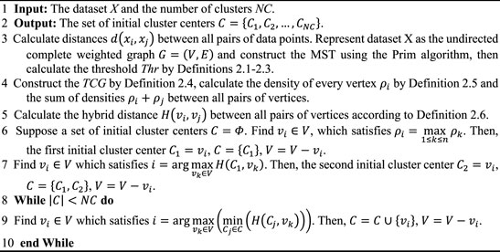
The Algorithm of the Proposed AIMK

Now we present the algorithm for determining the initial cluster centers based on the above-defined concepts. The details are as follows:

Algorithm 1 Algorithm of the proposed AIMK.

Algorithm Analysis

Clustering is NP-hard. No published optimization method provides theoretical guarantees for optimal partition of K-means for all datasets, even if the number of clusters is fixed to 2 (Dasgupta 2008). Due to the intractability of NP-hard problems, clustering algorithms are evaluated in terms of empirical performance on standard datasets. Therefore, in previous studies, many heuristic clustering algorithms have been proposed, one of the most well-known is clustering by fast search and find of density peaks (SFDP) (Rodriguez and Laio 2014). SFDP determines the cluster centers by measuring the two factors, the Gaussian kernel density of data points and the density-relative distance between data points. These two factors inspired the research of this paper. The proposed model is based on the skeleton points in the MST to estimate the density of each data point, and then combines the dissimilarity (i.e., distance) between the data points to calculate the hybrid distance matrix, and finally selects K data points, where the hybrid distances among them are relatively large, as the final cluster centers. In the experiment part, lots of test cases have demonstrated the effectiveness of the proposed model.

Time Complexity Analysis

According to the Algorithm 1, the time complexity of AIMK is analyzed as follows. In Step 3, the time complexity of computation of the distance between all pairs of vertices and the Prim algorithm is $\text{O}\left(n^2\right)$, and the time complexity of calculation of the threshold Thr is $O\left(n\right)$. Construction of the TCG and calculation of the density of every vertex ${\rho }_i$ requires $O\left(n\right)$ in Step 4, and the computation of the sum of densities ${\rho }_i+{\rho }_j$ between all pairs of vertices requires $O\left(n\right)$. In Step 5, because the distance and the sum of densities between all pairs of vertices have been obtained in Step 3 and Step 4, the time complexity of the calculation of the hybrid distance $H\left(v_i,v_j\right)$ between all pairs of vertices is $O\left(n\right)$. Determination of the first and second initial cluster centers requires $O\left(n\right)$ in Step 6 and Step 7. In Steps 8–10, the remaining initial cluster centers are selected, in which the time complexity is less than $NC\ast n$ and approximately equal to $O\left(NC\ast n\right)$. Because normally the number of clusters $NC\ll n$, the entire time complexity of AIMK is $\text{O}\left(n^2\right)$.

Reducing Complexity of AIMK by Sampling (AIMK-RS)

Due to the time complexity $O\left(n^2\right)$, it is difficult to apply AIMK to large or high-dimensional datasets. To solve this problem, we consider random sampling to extract $\sqrt{n}$ samples from the original dataset, where $n$ means the number of samples of the dataset, and then use these samples as the input for AIMK. It is worth mentioning that to make the $\sqrt{n}$ samples fully express the characteristics of the original dataset, we recommend using random sampling to reduce complexity only when the number of clusters $\text{K}\ll n$. In this way, the time complexity of AIMK will be reduced to $O\left(n\right)$. AIMK after random sampling, is denoted as AIMK-RS. The time complexities of all baselines (will be introduced in experiment part), AIMK and AIMK-RS are listed in Table 1.

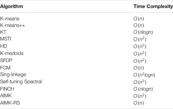
TABLE 1. Comparison of Time complexity.

Experiments

In this section, we mainly introduce the public datasets required for the experiment, well-known clustering algorithms, and several validation indices to evaluate the overall clustering performance and comparisons.

Datasets

In experiments, we use 22 real-world datasets (16 normal and six larger or higher-dimensional from the UCI Machine Learning Respository (https://archive.ics.uci.edu/ml/datasets) and LIBSVM official website (https://www.csie.ntu.edu.tw/∼cjlin/libsvmtools/datasets). The datasets include Breast-cancer, Shuttle, Pendigits, Colon-cancer, Zoo, Haberman, Svmguide2, Wine, Ionosphere, Leukemia, Gisette, Splice, Svmguide4, Liver-disorders, Soybean-small, Balance-scale, Ijcnn1, Phishing, Protein, Mushrooms, SensIT Vehicle (seismic), SensIT Vehicle (combined). The description of the datasets is as shown in Table 2.

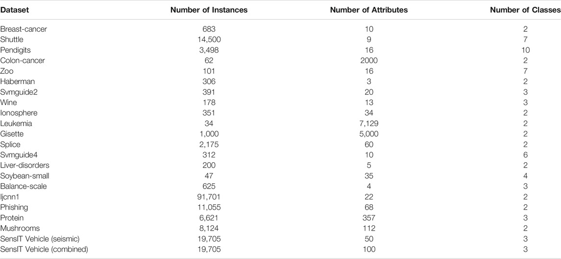
TABLE 2. Description of the 22 datasets.

State-of-The-Art Clustering Algorithms for Comparisons

We compare the clustering performance between AIMK and 11 selected clustering algorithms. For the sake of fairness, these baselines not only include initialization methods for K-means, such as K-means, K-means++, the method initializing K-means using kd-trees (KT) (Redmond and Heneghan 2007), the MST-based initializing K-means (MSTI) (Yang et al., 2017b), and the initialization method based on hybrid distance for K-means (HD) (Yang et al., 2017a), but also include some well-known clustering algorithms, such as K-medoids (Kaufman and Rousseeuw 2009), clustering by fast search and find of density peaks (SFDP) (Rodriguez and Laio 2014), fuzzy C-means clustering (FCM) (Bezdek et al., 1984), single-linkage hierarchical clustering (SH) (Johnson 1967), and self-tuning spectral clustering (SS) (Zelnik-Manor and Perona 2005), efficient parameter-free clustering using first neighbor relations (FINCH) (Sarfraz et al., 2019). Besides, since the results of K-means, K-means++, K-medoids, FCM, and SS are not unique, we take the average performance of 10 runs as the real performance. SFDP has a hyperparameter dc, ranging from 1–2% (Rodriguez and Laio 2014). We take the average performance while the hyperparameter equals 1, 1.1, 1.2, 1.3, 1.4, 1.5, 1.6, 1.7, 1.8, 1.9, and 2% because of the sensitivity of the hyperparameter. Furthermore, we take the ground-truth number of clusters as prior knowledge to choose the cluster centers in SFDP. For FINCH, we exploit the required number of clusters mode to ensure fairness of comparison. Note that all the baselines and AIMK used Euclidean distance as a metric. All experiments were performed in MatLab 2019b environment, and were conducted on a laptop with the 4-core Intel i7-10510U CPU clocked at 1.8 and 2.3 GHz and 16 GB memory.

Validation Indices

To evaluate the performance of clustering algorithms, we exploit three widely used external clustering validation indices including Accuracy (ACC), Rand Index (RI), and F-measure. These indices are defined as follows:

where n denotes the number of objects. NC is the number of clusters. P_i is the number of objects that are correctly assigned. TP means true positive, FP means false positive, FN means false negative, and TN means true negative (Powers 2011).

Results

In this section, we analyze the parameter setting of AIMK and then compare the proposed AIMK algorithm with other well-known clustering approaches. We then compare AIMK-RS with the two baselines with linear complexity on larger or higher-dimensional datasets. In addition, the AIMK is also applied to the variants of the K-means algorithm, K-medoids, and spectral clustering to prove the scalability.

Sensitivity and Setting of λ

To analyze the sensitivity of the parameter λ, we run AIMK on 16 datasets: Breast-cancer, Shuttle, Pendigits, Colon-cancer, Zoo, Haberman, Svmguide2, Wine, Ionosphere, Leukemia, Gisette, Splice, Svmguide4, Liver-disorders, Soybean-small, and Balance-scale while λ is set as 0, 0.25, 0.5, 0.75, 1. Then, we use ACC, RI, and F-measure to evaluate the performance of AIMK on each dataset. The results are listed in Tables 3–5. The optimal results for the corresponding index are denoted in bold. As the results show, when λ is set as 0 or 1, the optimal results in each validation index can be always obtained in each dataset. This is because of K-means’ own iterative mechanism. Even though different initial cluster centers are obtained because of different settings of the parameter λ, the same clustering results are finally obtained after iterating. The HD algorithm is required to run five times to obtain a better clustering result (Yang et al., 2017a), but AIMK can obtain a better result with only two runs, that is when λ is set as 0 or 1, respectively. Therefore, in subsequent experiments, we only consider the results of AIMK when λ equals 0 or 1.

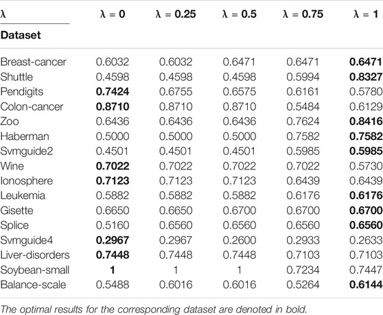
TABLE 3. AIMK Runs on 16 datasets, Measured by ACC.

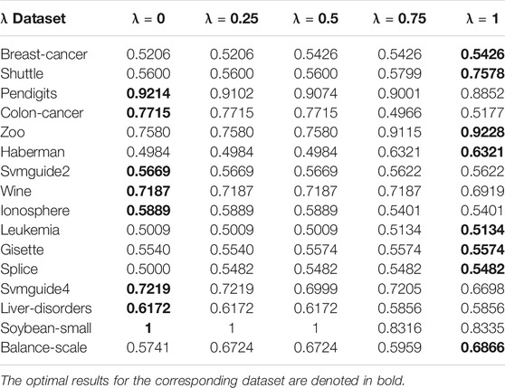
TABLE 4. AIMK Runs on 16 datasets, Measured by RI.

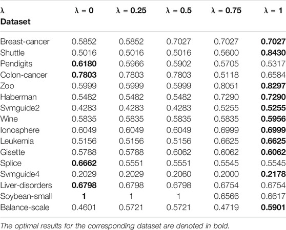
TABLE 5. AIMK Runs on 16 datasets, Measured by F-Measure.

Impact of Threshold Thr

To explain more clearly how to use skeleton points to determine the threshold Thr, we perform experiments on four representative datasets: Pendigits, Shuttle, Wine, and Gisette, whose data size and dimensions are from small to large and low to high, respectively. We run AIMK when Thr is set as the mean value of the maximum weights, mean weights, and minimum weights of adjacent edges of each skeleton point. Meanwhile, λ is set as 0 or 1, and the final results are shown as both sides of the slash “/’’, respectively. We use ACC to evaluate the results of each run. The results are shown in Table 6. For each dataset, the optimal results can be obtained only when Thr is set as the maximum weights of adjacent edges of each skeleton point. Therefore, it is more reasonable to set Thr as the maximum weights of adjacent edges of each skeleton point. Furthermore, the threshold Thr can be also used to help density-based clustering algorithms, such as DBSCAN (Ester et al., 1996), OPTICS (Ankerst et al., 1999), and SFDP, calculate the density of points without any extra adjusting parameters.

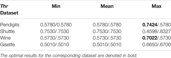
TABLE 6. The impact of Threshold Thr on clustering performance.

Comparison With Other Clustering Algorithms

We compare the clustering performance between AIMK (λ is set as 0 or 1) and 11 selected algorithms by 16 normal real-world datasets. ACC, RI, and F-measure are exploited to evaluate the performance of each baseline on each dataset. The results are listed in Tables 7–9. The optimal results for the corresponding dataset are denoted in bold. We use the average rank to measure the final performance of each baseline across datasets. The rank means the rank number of each row sorted in descending order. If there are the same results from two different algorithms, their ranks are equal.

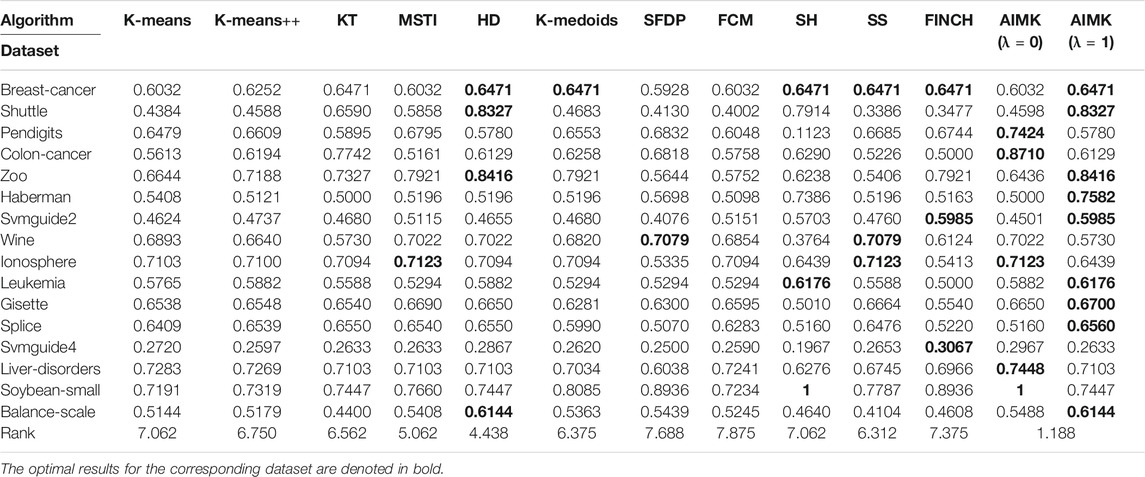
TABLE 7. Results of All Algorithms on 16 Real-World datasets, Measured by ACC.

According to Tables 7–9, AIMK (set λ as 0 or 1) achieves the best performance on 14, 13, and 8 of the 16 datasets when measured by ACC, RI, and F-measure, respectively. Moreover, it can be seen from the ranks that AIMK is obviously superior to the other 11 baselines, no matter which validation index we use.

Furthermore, according to Table 7, AIMK achieves the highest ACC rank compared with the other 11 baselines. The rank of AIMK 1.188 is much higher than the rank of HD 4.438, which achieves the second-highest ACC rank. FCM achieves the lowest ACC rank, at just 7.875. HD is the best-performing initialization method for K-means in addition to AIMK in Table 7, whose rank is 4.438. According to Table 8, AIMK achieves the highest RI rank compared with the other 11 baselines. The rank of AIMK 1.312 is much higher than the rank of HD 4.438, which achieves the second-highest RI rank. FINCH achieves the lowest RI, at just 9.000. HD is still the best-performing initialization method for K-means in addition to AIMK in Table 8, whose rank is 4.438. According to Table 9, AIMK still achieves the highest F-measure rank compared with the other 11 baselines. The rank of AIMK 1.938 is higher than the rank of SH 3.125, which achieves the second-highest F-measure rank. FCM achieves the lowest F-measure, which is just 10.00. MSTI is the best-performing initialization method for K-means in addition to AIMK in Table 9, whose rank is 5.938.

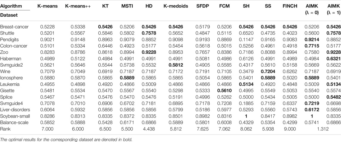
TABLE 8. Results of All Algorithms on 16 Real-World datasets, Measured by RI.

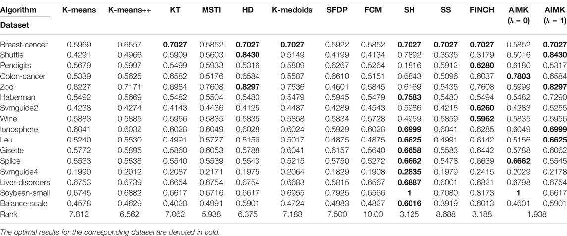
TABLE 9. Results of All Algorithms on 16 Real-World datasets, Measured by F-Measure.

To further investigate the statistical differences between the compared baselines and AIMK, we employ multiple comparisons with the best (MCB) test (Koning et al., 2005). The test computes the average ranks (in error rates, that is, 1-index values) of the forecasting methods according to the specific metric across all datasets of the competition and concludes whether or not these are statistically different. Figure 2 presents the results of the analysis. In addition, the Friedman p-values under the three indices (ACC, RI, and F-measure) are $1.48\times {10}^{-5}$, $1.1\times {10}^{-6}$ and $1.1\times {10}^{-11}$, respectively. Therefore, in a big picture, we can conclude AIMK provides significantly better performance than the other 11 compared baselines.

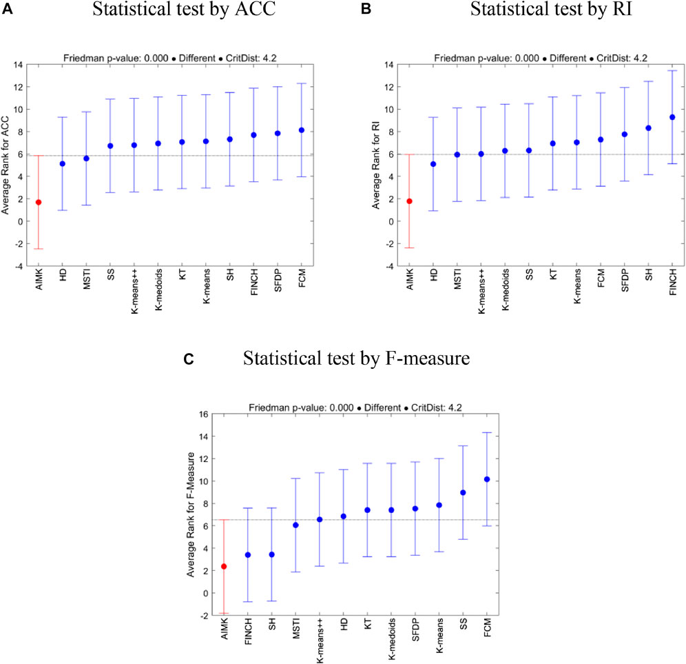
FIGURE 2. MCB test for AIMK and the compared baselines.

Performance of AIMK-RS

AIMK-RS is compared with two widely used initialization methods, K-means and K-means++, whose time complexity is also $O\left(n\right)$, on six larger or higher-dimensional datasets. ACC, RI, and F-measure are also exploited to evaluate the results. In addition, we take the average performance of 100 runs as the real performance of the AIMK-RS because it provides for more even sampling and can fully express the characteristics of the original datasets. The optimal results for the corresponding datasets are denoted in bold. The results are listed in Tables 10–12, and we can conclude that compared with the two baselines, AIMK-RS still achieves better performance. Particularly, on the dataset Ijcnn1, ACC, RI, and F-measure of AIMK-RS are increased by 7.68, 7.32, and 6.59%, respectively.

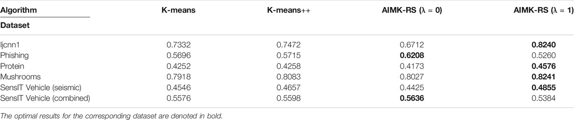
TABLE 10. Larger or Higher-Dimensional datasets, Measured by ACC.

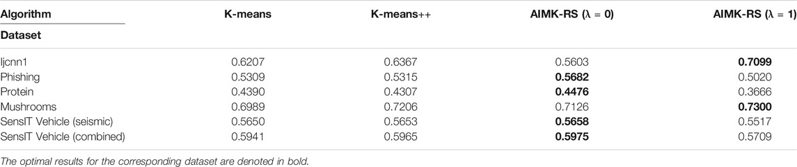
TABLE 11. Larger or Higher-Dimensional datasets, Measured by RI.

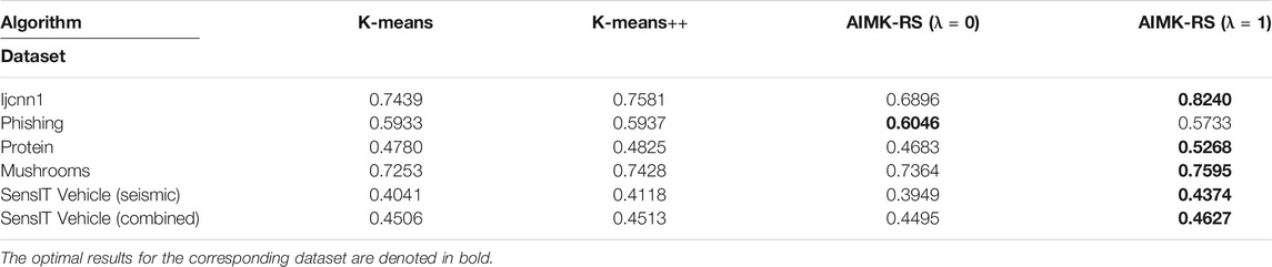
TABLE 12. Larger or Higher-Dimensional datasets, Measured by F-Measure.

Initialize Other Clustering Algorithms Using AIMK

In some variants of the K-means algorithm, the initialization method still plays an important role in the final clustering performance. For example, the initialization is required in the first step of the K-medoids algorithm and the last step of spectral clustering. However, the random initialization method is applied in the original algorithms. In this section, we even leverage AIMK to initialize the K-medoids clustering algorithm and spectral clustering algorithm. Due to the instability of original K-medoids and spectral clustering, we take the average performance of 10 runs as their real performance. There is a hyperparameter δ in the spectral clustering algorithm, so we use the self-tuning mode (Zelnik-Manor and Perona, 2005). The results are shown in Tables 13 and 14. In Table 13, the clustering performance of K-medoids initialized by AIMK, denoted as K-medoids + AIMK reaches the higher or equal performance on 15 datasets, except for the Gisette one. Particularly, the performance is increased by 36.44 and 8.39% on the Shuttle and Colon-cancer datasets, respectively. In Table 14, the overall higher clustering performance can be explored through spectral clustering initialized by AIMK, denoted as Spectral + AIMK. Especially Spectral + AIMK leads to 6.91 and 14.48% higher accuracy on the dataset Pendigits, Balance-scale, respectively.

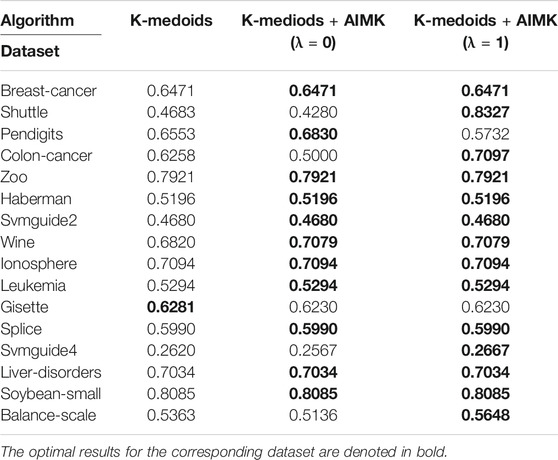
TABLE 13. Use AIMK to initialize the K-Medoids, measured by ACC.

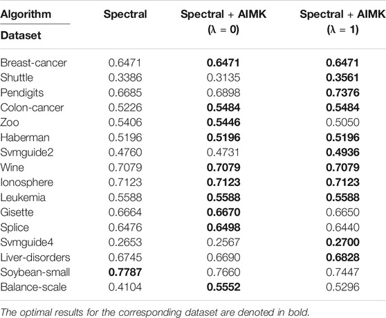
TABLE 14. Use AIMK to initialize spectral clustering, measured by ACC.

Discussion

Choice of λ

After the above experiments, we can see that the parameter λ is crucial for the final clustering results. To further illustrate the impact of parameter λ, we generate two types of datasets with different distributions from a mixture of three bivariate Gaussian densities. Figure 3A, Figure 3B is given by

FIGURE 3. To further illustrate the impact of parameter λ, we generate two types of datasets, (A), (B) and (C), (D), with different distribution from a mixture of three bivariate Gaussian densities. Class 1, Class 2, Class 3, and initial cluster centers are represented by different shapes: circle, cross, triangle, and star, respectively.

Figures 3C,D is given by $\frac{1}{3}Gaussian\left(\begin{array}{c}0\\ 0\end{array}\right)\left(\begin{array}{cc}0.01& 0\\ 0& 0.01\end{array}\right)+\frac{1}{3}Gaussian\left(\begin{array}{c}0\\ 0.6\end{array}\right)\left(\begin{array}{cc}0.01& 0\\ 0& 0.01\end{array}\right)+\frac{1}{3}Gaussian\left(\begin{array}{c}0.15\\ 0.15\end{array}\right)\left(\begin{array}{cc}0.01& 0\\ 0& 0.01\end{array}\right)$. where Gaussian (X, Y) is a Gaussian normal distribution with the mean X and the covariance matrix Y. We stimulate three clusters, namely, Class 1, Class 2 and Class 3, which are represented by different shapes: circle (20 points), cross (20 points), and triangle (20 points), respectively. As shown in Figures 3A–D, we use AIMK to determine the initial cluster centers marked with the star when λ is set as 0 and 1. In Figure 3A, Figure 3B, when λ is equal to 0, the three cluster centers happen to be the centroid of three classes. When λ is equal to 1, only one cluster center is the centroid of class 1, and the other two cluster centers are just outliers in class 2 and class 3, respectively. In Figure 3C, Figure 3D, when λ is equal to 0, two cluster centers are dropped in class 1, one cluster center is dropped in class 2, and no cluster center is dropped in class 3. However, when λ is equal to 1, three cluster centers happen to be dropped in three classes, and two of the three are outliers.

According to formula (Eq. 4), when λ is equal to 0, only the top K points with a higher density are selected as initial cluster centers. At this time, if all or most of these K initial cluster centers fall in K different classes, as shown in Figure 3A, then the initialization effect is better. However, for some datasets, such as overlapping datasets, shown as Figure 3C, the top K points with higher density cannot be distributed relatively evenly among K classes. Therefore, at this time, we need to consider the distance factor. According to formula (Eq. 4), when λ is equal to 1, we only select the K points that are far apart from each other as initial cluster centers. At this time, all or most of these K initial cluster centers are more likely to be relatively evenly distributed among the K classes, as shown in Figure 3D.

In summary, if the users have prior knowledge of the datasets, the parameter λ can be selected more accurately like the examples above in advance. Otherwise, they can still get good clustering results by executing the algorithm in just two interactions.

Conclusion

In this study, we propose the AIMK algorithm which can not only adapt to datasets with various characteristics but also obtain better clustering results within two runs. First, we propose a new threshold to calculate the density of the data points based on the skeleton points of MST. Second, we compute the hybrid distances based on the density of the data points. Finally, we select K data points, where the hybrid distances among them are relatively large, as the final cluster centers. In addition, we apply random sampling to AIMK to obtain the AIMK-RS, whose time complexity is only O(n).

In the experiment part, first, we analyze the sensitivity of parameter λ on each dataset, and conclude that better performance can be obtained when λ is 0 or 1. Second, we compare AIMK with 11 different algorithms on 16 normal datasets. The experimental results show that AIMK outperforms the current initialization methods and several well-known clustering algorithms. We also compare AIMK-RS with two widely used initialization methods with linear complexity. AIMK-RS still achieves better performance. Particularly, the ACC, RI, and F-measure are increased by 7.68, 7.32, and 6.59% on the dataset Ijcnn1, respectively. Finally, we exploit AIMK to initialize the variants of K-means, such as K-medoids and spectral clustering. The better clustering performance demonstrates AIMK is a good way for initialization and has the potential to extend to other state-of-the-art algorithms. Particularly, for the K-medoids initialized by AIMK, the performance is increased by 36.44 and 8.39% on the Shuttle and Colon-cancer datasets, respectively. Similarly, spectral clustering initialized by AIMK leads to 6.91 and 14.48% higher accuracy on the dataset Pendigits, Balance-scale, respectively. In the discussion part, we take two toy examples to show the choice of λ for datasets with different characteristics.

In the future, we will combine AIMK or AIMK-RS with other state-of-art algorithms to more real-world datasets. Moreover, we will leverage them to some specific applications, such as image segmentation, classification of EEG data, etc.

Data Availability Statement

The datasets generated for this study are available on request to the corresponding author or Jie Yang (jie.yang-4@student.uts.edu.au).

Author Contributions

JY developed the methodology, performed the experiments, and wrote the manuscript. Y-KW, XY and C-TL gave important suggestions for designing the research and writing the manuscript. The research was supervised by Y-KW and C-TL.

Funding

This work was supported in part by the Australian Research Council (ARC) under discovery grant DP180100656 and DP210101093. Research was also sponsored in part by the Australia Defence Innovation Hub under Contract No. P18-650825, US Office of Naval Research Global under Cooperative Agreement Number ONRG - NICOP - N62909-19-1-2058, and AFOSR – DST Australian Autonomy Initiative agreement ID10134. We also thank the NSW Defence Innovation Network and NSW State Government of Australia for financial support in part of this research through grant DINPP2019 S1-03/09 and PP21-22.03.02.

Conflict of Interest

The authors declare that the research was conducted in the absence of any commercial or financial relationships that could be construed as a potential conflict of interest.

Publisher’s Note

All claims expressed in this article are solely those of the authors and do not necessarily represent those of their affiliated organizations, or those of the publisher, the editors, and the reviewers. Any product that may be evaluated in this article, or claim that may be made by its manufacturer, is not guaranteed or endorsed by the publisher.

Acknowledgments

We also thank the support from PengCheng Professorship. We also thank the NSW Defence Innovation Network and NSW State Government of Australia for financial support in part of this research through grant DINPP2019 S1-03/09 and PP21-22.03.02.

References

Anerst, M., Breunig, M. M., Kriegel, H.-P., and Sander, J. (1999). “OPTICS: Ordering Points to Identify the Clustering Structure,” in SIGMOD 99: Proceedings of the 1999 ACM SIGMOD International Conference on Management of Data, Philadelphia, PA, 49–60. doi:10.1145/304181.304187
Arthur, D., and Vassilvitskii, S. (2007). “K-Means++: The Advantages of Careful Seeding,” in Proceedings of the Eighteenth Annual ACM-SIAM Symposium on Discrete Algorithms, New Orleans, Louisiana, January 7–9, 2007 (Society for Industrial and Applied Mathematics), 1027–1035.
Bezdek, J. C., Ehrlich, R., and Full, W. (1984). FCM: The Fuzzy C-Means Clustering Algorithm. Comput. Geosci. 10 (2–3), 191–203. doi:10.1016/0098-3004(84)90020-7
Bu, Z., Li, H.-J., Zhang, C., Cao, J., Li, A., and Shi, Y. (2020). Graph K-Means Based on Leader Identification, Dynamic Game, and Opinion Dynamics. IEEE Trans. Knowl. Data Eng. 32, 1348–1361. doi:10.1109/TKDE.2019.2903712
Cao, F., Liang, J., and Jiang, G. (2009). An Initialization Method for the K-Means Algorithm Using Neighborhood Model. Comput. Maths. Appl. 58 (3), 474–483. doi:10.1016/j.camwa.2009.04.017
Chang, H.-J., Hung, L.-P., and Ho, C.-L. (2007). An Anticipation Model of Potential Customers' Purchasing Behavior Based on Clustering Analysis and Association Rules Analysis. Expert Syst. Appl. 32 (3), 753–764. doi:10.1016/j.eswa.2006.01.049
Connell, S. D., and Jain, A. K. (1998). “Learning Prototypes for Online Handwritten Digits,” in Proceedings. Fourteenth International Conference on Pattern Recognition (Cat. No.98EX170), Brisbane, QLD, Australia, 20–20 Aug 1998 182–184. doi:10.1109/ICPR.1998.711110
Dasgupta, S. (2008). The Hardness of K-Means Clustering. Technical Report CS2008-0916. Available at: https://www.semanticscholar.org/paper/The-hardness-of-k-means-clustering-Dasgupta/426376311a7526bd77dacd27fd1a7d58dc2da7e1 (Accessed June 30, 2021).
Dorai, C., and Jain, A. K. (1995). “Shape Spectra Based View Grouping for Free-form Objects,” in Proceedings: International Conference on Image Processing, Washington, DC, USA, 23–26 Oct 1995, 340–343. doi:10.1109/ICIP.1995.538548
Ester, M., Kriegel, H. P., and Xu, X. (1996). “A Density-Based Algorithm for Discovering Clusters in Large Spatial Databases with Noise,” in KDD'96: Proceedings of the Second International Conference on Knowledge Discovery and Data Mining, Portland, Oregon, August 2–4, 1996, 226–231.
Forgy, E. W. (1965). Cluster Analysis of Multivariate Data : Efficiency versus Interpretability of Classifications. Biometrics 21, 768–769.
Gonzalez, T. F. (1985). Clustering to Minimize the Maximum Intercluster Distance. Theor. Comput. Sci. 38 (January), 293–306. doi:10.1016/0304-3975(85)90224-5
Huang, Z. (1997). A Fast Clustering Algorithm to Cluster Very Large Categorical Data Sets in Data Mining. DMKD 3 (8), 34–39.
Jancey, R. (1966). Multidimensional Group Analysis. Aust. J. Bot. 14 (1), 127–130. doi:10.1071/bt9660127
Jiang, D., Chen, G., Ooi, B. C., Tan, K.-L., and Wu, S. (2014). “epiC,” in Proceedings of the VLDB Endowment, Hangzhou, China, September 1st–5th 2014, 541–552. doi:10.14778/2732286.2732291
Johnson, S. C. (1967). Hierarchical Clustering Schemes. Psychometrika 32 (3), 241–254. doi:10.1007/BF02289588
Kaufman, L., and Rousseeuw, P. J. (2009). Finding Groups in Data: An Introduction to Cluster Analysis, Vol. 344. New York: John Wiley & Sons.
Khan, I., Luo, Z., Huang, J. Z., and Shahzad, W. (2020). Variable Weighting in Fuzzy K-Means Clustering to Determine the Number of Clusters. IEEE Trans. Knowl. Data Eng. 32, 1838–1853. doi:10.1109/TKDE.2019.2911582
Khan, S. S., and Ahmad., A. (2004). Cluster Center Initialization Algorithm for K-Means Clustering. Pattern Recognition Lett. 25 (11), 1293–1302. doi:10.1016/j.patrec.2004.04.007
Kiselev, V. Y., Andrews, T. S., and Hemberg, M. (2019). Challenges in Unsupervised Clustering of Single-Cell RNA-Seq Data. Nat. Rev. Genet. 20 (5), 273–282. doi:10.1038/s41576-018-0088-9
Koning, A. J., Franses, P. H., Hibon, M., and Stekler, H. O. (2005). The M3 Competition: Statistical Tests of the Results. Int. J. Forecast. 21 (3), 397–409. doi:10.1016/j.ijforecast.2004.10.003
Lai, Y., He, S., Lin, Z., Yang, F., Zhou, Q.-F., and Zhou, X. (2020). An Adaptive Robust Semi-supervised Clustering Framework Using Weighted Consensus of Random K-Means Ensemble. IEEE Trans. Knowl. Data Eng. 1, 1. doi:10.1109/TKDE.2019.2952596
MacQueen, J. (1967). “Some Methods for Classification and Analysis of Multivariate Observations,” in Proceedings of the Fifth Berkeley Symposium on Mathematical Statistics and Probability, Oakland, CA, USA, 281–297.
Manochandar, S., Punniyamoorthy, M., and Jeyachitra, R. K. (2020). Development of New Seed with Modified Validity Measures for K-Means Clustering. Comput. Ind. Eng. 141 (March), 106290. doi:10.1016/j.cie.2020.106290
Murugesan, V. P., and Punniyamoorthy, M. (2020). A New Initialization and Performance Measure for the Rough K-Means Clustering. Soft Comput. 24 (15), 11605–11619. doi:10.1007/s00500-019-04625-9
Powers, D. M. (2011). Evaluation: From Precision, Recall and F-Measure to ROC, Informedness, Markedness and Correlation. J. Machine Learn. Tech. 2 (1), 37–63. doi:10.9735/2229-3981
Prim, R. C. (1957). Shortest Connection Networks and Some Generalizations. Bell Syst. Tech. J. 36 (6), 1389–1401. doi:10.1002/j.1538-7305.1957.tb01515.x
Redmond, S. J., and Heneghan, C. (2007). A Method for Initialising the K-Means Clustering Algorithm Using Kd-Trees. Pattern Recognition Lett. 28 (8), 965–973. doi:10.1016/j.patrec.2007.01.001
Rodriguez, A., and Laio, A. (2014). Clustering by Fast Search and Find of Density Peaks. Science 344 (6191), 1492–1496. doi:10.1126/science.1242072
Sarfraz, S., Sharma, V., and Stiefelhagen, R. (2019). “Efficient Parameter-free Clustering Using First Neighbor Relations,” in 2019 IEEE/CVF Conference on Computer Vision and Pattern Recognition (CVPR), Long Beach, CA, USA, June 16th–June 20th, 2019, 8926–8935. doi:10.1109/CVPR.2019.00914
Saxena, A., Prasad, M., Gupta, A., Bharill, N., Patel, O. P., Tiwari, A., et al. (2017). A Review of Clustering Techniques and Developments. Neurocomputing 267 (December), 664–681. doi:10.1016/j.neucom.2017.06.053
Shah, S. A., and Koltun, V. (2017). Robust Continuous Clustering. Proc. Natl. Acad. Sci. USA 114 (37), 9814–9819. doi:10.1073/pnas.1700770114
Wang, Y., Li, C., and Zuo, Y. (2009). A Selection Model for Optimal Fuzzy Clustering Algorithm and Number of Clusters Based on Competitive Comprehensive Fuzzy Evaluation. IEEE Trans. Fuzzy Syst. 17 (3), 568–577. doi:10.1109/TFUZZ.2008.928601
Yang, J., Ma, Y., Zhang, X., Li, S., and Zhang, Y. (2017b). A Minimum Spanning Tree-Based Method for Initializing the K-Means Clustering Algorithm. Int. J. Comput. Inf. Eng. 11, 13–17. doi:10.5281/zenodo.1128109
Yang, J., Ma, Y., Zhang, X., Li, S., and Zhang, Y. (2017a). An Initialization Method Based on Hybrid Distance for K-Means Algorithm. Neural Comput. 29 (11), 3094–3117. doi:10.1162/neco_a_01014
Zelnik-Manor, L., and Perona, P. (2005). “Self-Tuning Spectral Clustering,” in Advances in Neural Information Processing Systems. Editors L. K. Saul, Y. Weiss, and L. Bottou (Vancouver British Columbia, Canada: MIT Press), 1601–1608.
Keywords: k-means, adaptive, initialization method, initial cluster centers, clustering
Citation: Yang J, Wang Y-K, Yao X and Lin C-T (2021) Adaptive Initialization Method for K-Means Algorithm. Front. Artif. Intell. 4:740817. doi: 10.3389/frai.2021.740817
Received: 13 July 2021; Accepted: 25 October 2021;
Published: 25 November 2021.
Edited by:
Mohammad Akbari, Amirkabir University of Technology, IranReviewed by:
Yugal Kumar, Jaypee University of Information Technology, IndiaRoshan Chitrakar, Nepal College of Information Technology, Nepal
Copyright © 2021 Yang, Wang, Yao and Lin. This is an open-access article distributed under the terms of the Creative Commons Attribution License (CC BY). The use, distribution or reproduction in other forums is permitted, provided the original author(s) and the copyright owner(s) are credited and that the original publication in this journal is cited, in accordance with accepted academic practice. No use, distribution or reproduction is permitted which does not comply with these terms.
*Correspondence: Chin-Teng Lin, Chin-Teng.Lin@uts.edu.au