Internal wave activity in the deep Gulf of Mexico

1 Introduction

The Gulf of Mexico (GoM) is a semi-enclosed basin connected to the Caribbean Sea through the Yucatan Channel and to the south-western North Atlantic through the Florida Strait. The eastern GoM’s circulation is dominated by the Loop Current (LC) (Austin and George, 1955; Sturges and Evans, 1983; Leben, 2005), which connects the two straits and carries warm and salty subtropical underwater (SUW) between the surface and ≈ 300 m and Tropical Atlantic Central Water (TACW) between 300 m and the approximate depth of the Florida Sill (≈740 m) (Hamilton et al., 2018; Portela et al., 2018). The LC was named after the large loop it makes in the eastern GoM, consisting of a pool of lighter water (SUW and TACW) yielding an anticyclonic circulation. The LC extension is highly variable from a fully retracted mode, known as the port to port mode, where the flow directly links the two channels in a nearly straight line along the Northern slope of Cuba, and an extended mode where the tip of the LC reaches the Texas Louisiana continental shelf to the north (Leben, 2005; Oey et al., 2005). While the growth of the LC from retracted to fully extended mode is a slow process and takes about a year, the transition from extended to retracted modes can be quite sudden as a large warm core ring detaches from the LC. Meandering of the LC’s edge also participates in the variability of its position (Donohue et al., 2016a; Donohue et al., 2016b). It is important to note that the usual LC terminology does not only designate the fast current associated with the sharp front between SUW and the Gulf Common Water (GCW), but also embodies the whole SUW water mass bounded by the front. In this work, we follow this common terminology and when we refer to the LC, we refer to this whole warm water-mass, which is also associated with a large anticyclonic circulation.

Beneath the TACW, between ≈ 700 and 900 m lies a layer of Antarctic intermediate water (AAIW) stacked over a large volume of North Atlantic deep water (NADW) that occupies the lower layer of the GoM between 1200 m and the bottom (≈3800 m at its deepest) (Rivas et al., 2005; Portela et al., 2018). Since the depth of the sill is much deeper in the Yucatan Channel than in the Florida Strait (2000 and 740 m, respectively), water entering the GoM below 740 m does not exit through the Florida Strait. As the GoM extends to much greater depths than the Yucatan Channel, which represents the only entrance for external water, the ventilation process of the deep GoM is of particular interest. It is dominated by sporadic events of inflow of slightly colder NADW from the Caribbean (compared to GoM’s NADW), that last a few days to a few weeks (Rivas et al., 2005). This inflow occurs in the bottom 200 m of the sill and the NADW then, once it enters the Gulf, sinks under the lighter GoM’s water until it reaches the bottom. Using moored ADCP and CTD data, Rivas et al. (2005) estimated that the time necessary for the renewal of the full NADW deep layer (residence time) was of about 250 years (later confirmed by ¹4C measurements of Chapman et al. (2018)), while Amon et al. (2023)’s ¹4C measurements suggest a much shorter residence time of ≈ 100 years, in agreement with Ochoa et al. (2021)’s results based on heat balance.

Because ventilation events require the GoM’s water to be warmer than the inflow water at the sill depth and all levels below, and that cold inflow water is the only source of external water, some process must be invoked for the warming of the deep GoM, such as diapycnal mixing. Oxygen distribution in the GoM also supports the necessity of some vertical diffusivity to occur in the deep GoM. NADW is a particularly oxygen-rich water mass ([4-6] ml l⁻¹) compared to the overlying AAIW, TACW and SUW (≈ [3-4], [2.5-3.5], and [3-3.5] ml l⁻¹, respectively) (Portela et al., 2018). Remarkably, Nowlin and McLellan (1967); Rivas et al. (2005) and Amon et al. (2023) noted that below 1000 m, the oxygen concentration in the GoM decreases with increasing distance from the Yucatan Channel. At shallower depths, the situation is reversed, and the oxygen concentration increases away from the Yucatan Channel, consistent with mixing of the two layers. Combining the observations of a series of ship surveys using CTD, ADCP and oxygen measurements with a mooring array in the Yucatan Channel, Rivas et al. (2005) computed a full oxygen budget for the GoM, and concluded that oxygen consumption was not sufficient to balance the advective flux through the Yucatan Channel, so that significant vertical diffusivity has to be invoked to close the oxygen budget. Recently, Ochoa et al. (2021) proposed a conceptual model for the warming of the deep GoM, consisting in a diffusive upwelling on the continental slopes in the form of diapycnal mixing. Using glider observations of microstructure, Molodtsov et al. (submitted manuscript) measured elevated levels of turbulent kinetic energy over the western continental slopes and proposed that internal waves might act as the necessary sources of diapycnal mixing.

The internal waves – a variety of oceanic oscillations with frequencies ranging from the inertial (f) and buoyancy (N) frequencies – are thought to provide the main path for energy dissipation in the World Ocean through a forward energy cascade driven by wave-wave interactions (Polzin et al., 1995; Polzin et al., 2014). In the spectral domain, these interactions result in a “continuum” of internal waves which can be modelled by the well-known GM spectrum (Garrett and Munk, 1975) for which both spectral slope and energy level are constant. While the forward energy cascade and the associated processes [e.g., wave triads; McComas and Bretherton (1977)] are not fully understood, the link between internal wave activity (i.e., spectral level and slope) and the turbulent dissipation of kinetic energy (ϵ) yielding diapycnal mixing is well-attested (Gregg, 1989; Polzin et al., 2014; Whalen et al., 2015).

The main energy sources for the internal waves continuum are the near-inertial waves generated by the wind, topographic interaction with geostrophic current and mesoscale fronts (Alford et al., 2016), and the internal tides forced by barotropic tides at locations where the bottom slope matches the wave slope. In addition to these energy sources, high internal wave modes can be generated near the bottom when large-scale features (e.g., mesoscale eddies) interact with rough topographies (Clément et al., 2016). These energy sources modify the shapes of the internal wave spectra (e.g., kinetic and potential energy spectra, shear and strain spectra) at the wavenumbers and frequencies where the energy is injected and are likely to modify the rest of the internal wave continuum (Le Boyer and Alford, 2021) as they impact the forward energy cascade through wave-wave interactions.

Previous studies have investigated the dynamics of internal waves in the Northern GoM, showing an energy transfer from low-frequency (balanced) flows into the internal wave field, particularly near the inertial frequency (Jing et al., 2018). The role of Hurricane wakes in internal wave generation was also shown to be important both in the Northern GoM (Jing et al., 2015) and near the LC region (Pallàs-Sanz et al., 2016a; Pallàs-Sanz et al., 2016b). Interestingly, Jing et al. (2015) showed that these internal waves in the Northern GoM were associated with elevated diapycnal mixing. However, these regional studies based on mooring observations were restricted to the upper layers of the GoM, and could not highlight the properties of the internal wave field in the deep GoM, where the mixing of the NADW with the overlying AAIW should occur.

In this work, we aim to characterize the geographical distribution of internal waves activity in the deep eastern GoM, north of the Yucatan Channel, using a fleet of profiling floats that continuously measure temperature, salinity and pressure as they drift. Following Hennon et al. (2014), time series of temperature are converted into isopycnal displacements. The floats drift at 1500 dbar, in the upper limit of the NADW, only a few hundred meters above the Yucatan Sill and below the overlying AAIW layer, where diapycnal mixing would be expected to play an important role in warming the bottom layer and reducing its oxygen content. Although estimates of turbulent diffusivity in the region would be of interest to directly assess the impact of internal waves on water masses mixing, the profiling floats data set does not allow us to perform such estimates accurately. While fine-scale strain parameterizations have proven to be powerful tools in estimating turbulent diffusivity (Kunze et al., 2006; Thompson et al., 2007), and were applied to Argo float profiles in the past (Whalen et al., 2012; Whalen et al., 2015), the GoM’s stratification at our depth of interest is particularly weak, so that vertical strain estimates essentially result in noise, considering the float’s thermistor and conductivity cell precision. This study only focuses on characterizing the geography of the internal wave activity in terms of isopycnal displacement and available potential energy and does not provide estimates of the resulting turbulent diffusivity.

The profiling floats dataset is described in section 2.1 and the isopycnal displacement reconstruction methods and calculations of available potential energy are detailed in section 2.2. The geographical distribution of internal wave properties is described in section 3.1 and the driving processes are studied in section 3.2. The results are then discussed in section 4.

2 Data and methods

2.1 Profiling float observations

Since June 2019, 29 Solo autonomous profilers have been sampling the Eastern Gulf of Mexico in the LC region. These floats have the particularity of drifting at ≈1500 dbar, profile every five days, and continuously measure pressure, conductivity, and temperature at an hourly rate as they drift at the parking depth. The average float displacement between two surfacings is of ≈26 km and 99.9% of these displacements were smaller than 1°. As of November 2022, the floats have collected 5781 vertical profiles and time series of temperature and salinity during drift phases. Here, both the vertical profiles and the drift-phase observations are used to infer isopycnal displacement time series. For the consistency of the dataset, only floats freely drifting between 1400 and 1600 dbar were used and all data from floats bumping against the bottom on the continental slopes were removed. After applying this criterion, along with a strict quality control of the data, 2615 profiles and time series were retained. The profiles locations are shown in Figure 1A, and the number of observations per 0.5° ×0.5° grid points is shown in Figure 1B. The position of the Loop Current was detected using AVISO absolute dynamic topography (ADT; thereafter referred to as SSH). Its edge is defined by the minimum value SSH contour passing through both the Yucatan Channel and the Florida Strait. On average, this corresponds to the 50 cm SSH isopleth. The probability of the presence of the LC in the eastern GoM is shown as a color-map in Figure 1A. A vast majority of the profiles (and time series) were collected in the region of influence of the Loop Current.

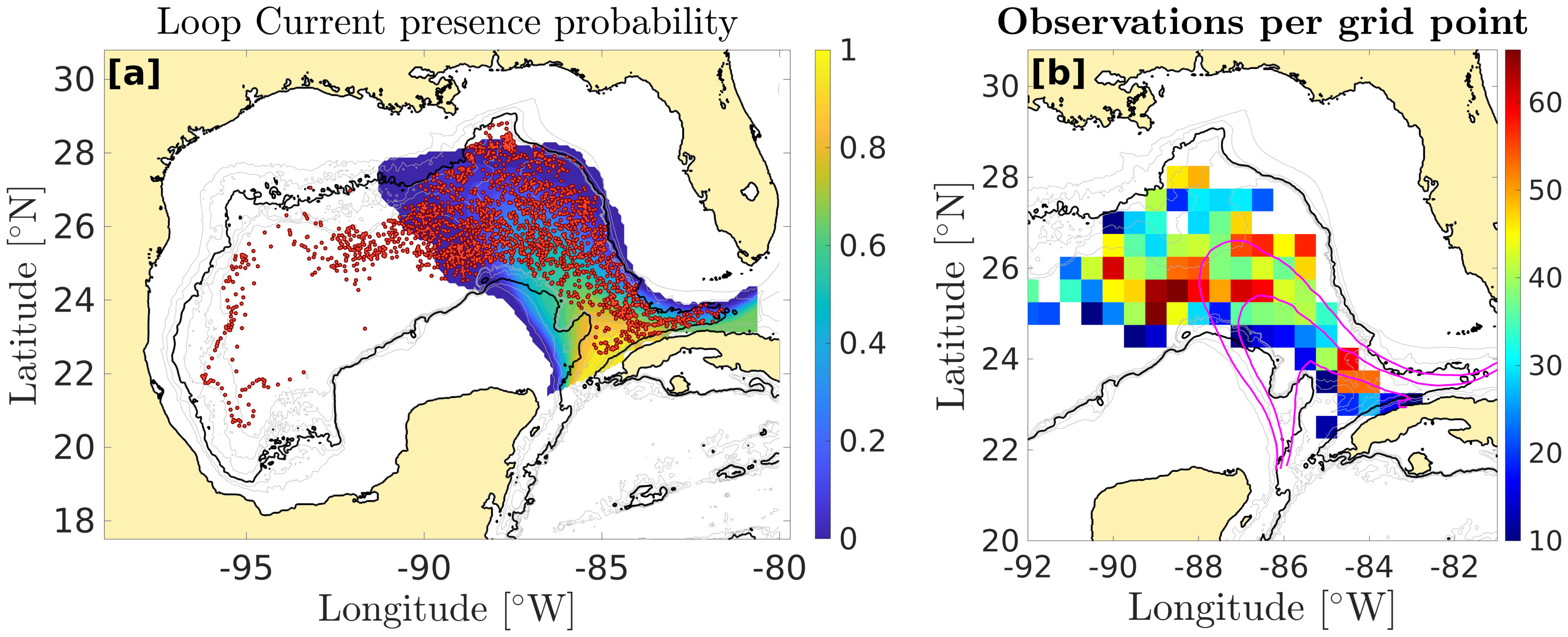
Figure 1 (A) Probability of the presence of the Loop Current (LC) between June 2019 and March 2023. The LC’s edge is the outermost absolute dynamic topography (SSH) contour passing through the Yucatan Channel and the Florida Strait. The red dots represent the locations of the float profiles. (B) Number of observations per grid point in the ${\frac{1}{2}}^{°}$ gridded Gulf of Mexico. The magenta contours represent the Loop Current presence probability. The outtermost contour is 0.1, the middle contour is 0.5, and the southernmost contour is 0.9.

Because stratification is weak in the GoM near the floats’ parking depth, the lack of precision of the salinity measurements may introduce significant noise that needs to be addressed. Figure 2A shows 50 m low-passed filtered vertical salinity profiles for the entire dataset between 1200 and 1800 dbar, along with the pressure and salinity values observed during the drift phases. Figure 2B shows a T-S plot for the same pressure range. On average, salinity varies by less than 0.03 psu between 1200 and 1800 dbar. Salinity measurements at the parking depth also have a narrow range, between 34.95 and 34.98 psu, while the precision of salinity measurements of standard Argo floats is estimated to be 0.01 psu. On the other hand, the temperature range at the parking depth is ≈0.2°C, 100 times the estimated Argo’s Sea-bird SBE 41 thermistor’s precision, so that temperature measurements can be considered as reliable at these depths. The lack of precision of the salinity measurements is evident in the randomly selected profiles of Figure 2C and d as staircase patterns, where salinity only takes discrete values. An example of time series of the temperature and salinity contribution to density anomaly during the drift phase is also shown in Figure 3A. The lack of resolution in the salinity measurement is particularly evident as a seemingly random shift between two discrete values, while the temperature is well resolved. Variance spectra were computed for density anomaly and the contributions of temperature (σ₀(αT^′), where α is the thermal expansion coefficient) and salinity (σ₀(βS^′), where β is the haline contraction coefficient) (Figure 3B). The spectrum associated with the raw salinity is nearly flat between 4 and 10 cpd (≈ ω⁻⁰.³), while the temperature spectrum is much steeper (≈ ω⁻¹.⁷), showing that the raw salinity signal in the time series is essentially noise. Despite this noise in salinity measurements, a clear linear relationship between temperature and salinity is evident in Figure 2D, so that salinity can be recovered from temperature measurements using linear regression. The corrected salinity inferred from temperature is shown in Figures 2C, D. After correcting salinity, the spectrum recovers the slope of the temperature spectrum (Figure 3B). Consequently, the density spectrum computed using corrected salinity is also steeper than raw density, consistent with a strong noise reduction at high frequency. Corrected salinity, based on temperature, is used throughout this paper.

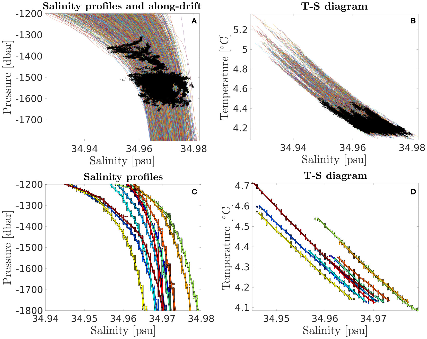
Figure 2 (A) Salinity against pressure between 1200 and 1800 dbar for all the vertical profiles (colored lines) and for the drift phase time series (black dots). (B) T-S diagram using the same data as in (A). (C) Raw (dots) and corrected (continuous lines) salinity profiles for 12 randomly selected vertical profiles. The seemingly straight vertical lines crossing the profiles are contiguous dots representing the raw data (D) same as (C) for the T-S diagram.

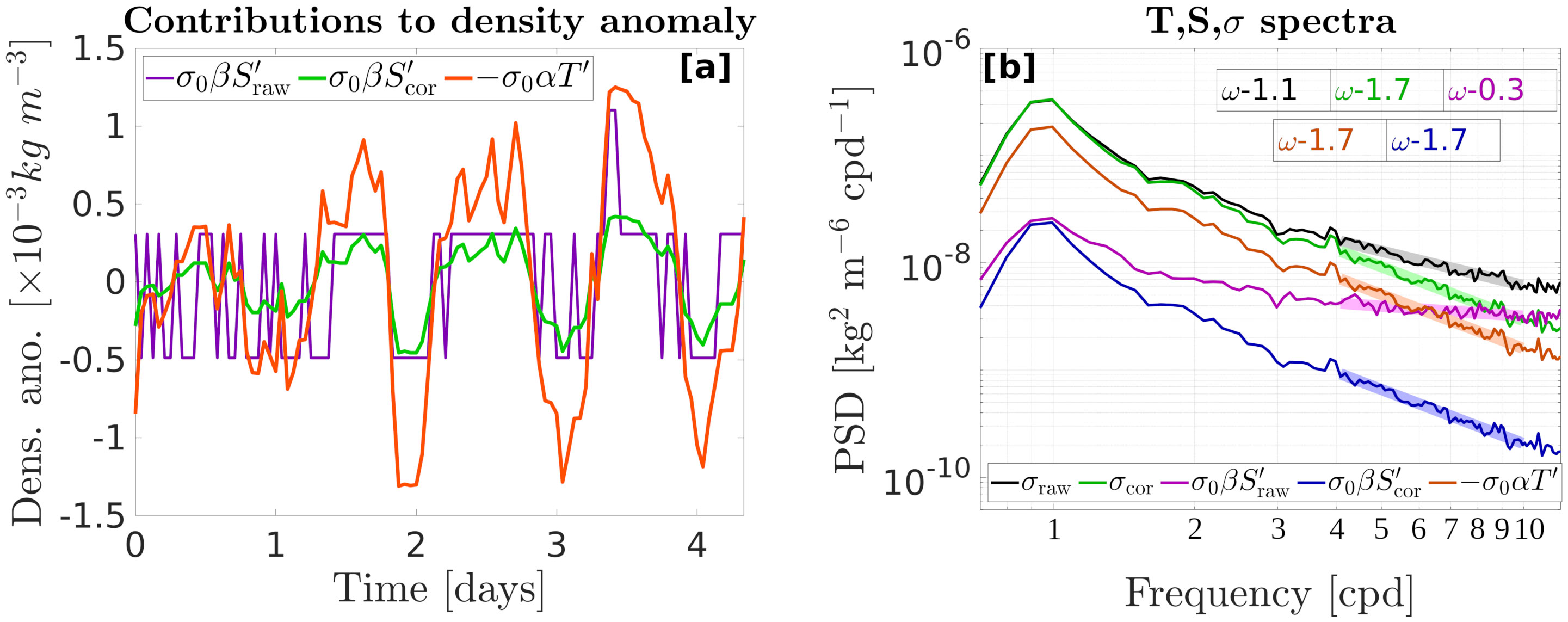
Figure 3 (A) Time series of temperature and salinity contributions to the density anomaly. The orange line represents temperature, the magenta line represents raw salinity, and the green line represents corrected salinity. (B) Power spectral density of density anomaly and temperature and salinity contributions. The black line is the density computed from the raw salinity data, the green line is the density computed with the corrected salinity, the magenta line is the raw salinity contribution to density anomaly, the blue line is the corrected salinity contribution, and the orange line is temperature contribution to density anomaly. The spectral slopes indicated in the text boxes were computed between 4 and 10 cycles per day (cpd).

2.2 Isopycnal displacements reconstruction

Isopycnal displacements are first estimated from the pressure and corrected potential density (hereafter density) time series during the drift phase (p_d(t) and σ_d(t), respectively), using the previous and next vertical density profiles to construct a reference mean state σ_r(z). For each measurement of the time series, we define the equivalent pressure p_e(t) as the pressure of the density value σ_d(t) in the reference profile σ_r(z). The displacement is then defined as the difference between the observed pressure and the equivalent pressure: η(t) = p_d(t)− p_e(t). In the case of linear stratification ($\frac{d{\sigma }_r}{dp}=\gamma$, where γ  is a constant), Hennon et al. (2014) showed that the isopycnal displacement could be inferred as:

Although linear stratification is not required to infer isopycnal displacements, since the method first described in this section is valid for any stratification, it is convenient if we want to discuss the available potential energy (APE) associated with the internal wave field. When the Buoyancy frequency is constant, APE is proportional to the squared isopycnal displacement (Polzin and Lvov, 2011):

where ${\sigma }_0$ is a reference density and $N^2$ is the squared buoyancy frequency, defined as:

APE is thus proportional to the squared buoyancy frequency-scaled (BFS) isopycnal displacement $\tilde{\eta }(t)$:

where N₀ is a reference buoyancy frequency. Although N₀ could be any arbitrary value, here we define it as the average buoyancy frequency of all available vertical profiles at the parking depth in the GoM.

To assess the validity of the linear stratification approximation, we performed a linear regression on each reference density profile over the pressure range spanned by the equivalent pressure p_e(t) of the corresponding time series. A quadratic fit was also computed for comparison. Figure 4A shows the coefficient of determination (R²) for each fit. The quadratic fit is an excellent approximation, with a mean R² > 0.998, and no value below 0.99. The linear approximation, despite lower R² values, is also a solid estimate of the density profiles, with an average R² greater than 0.99 and no value below 0.94.

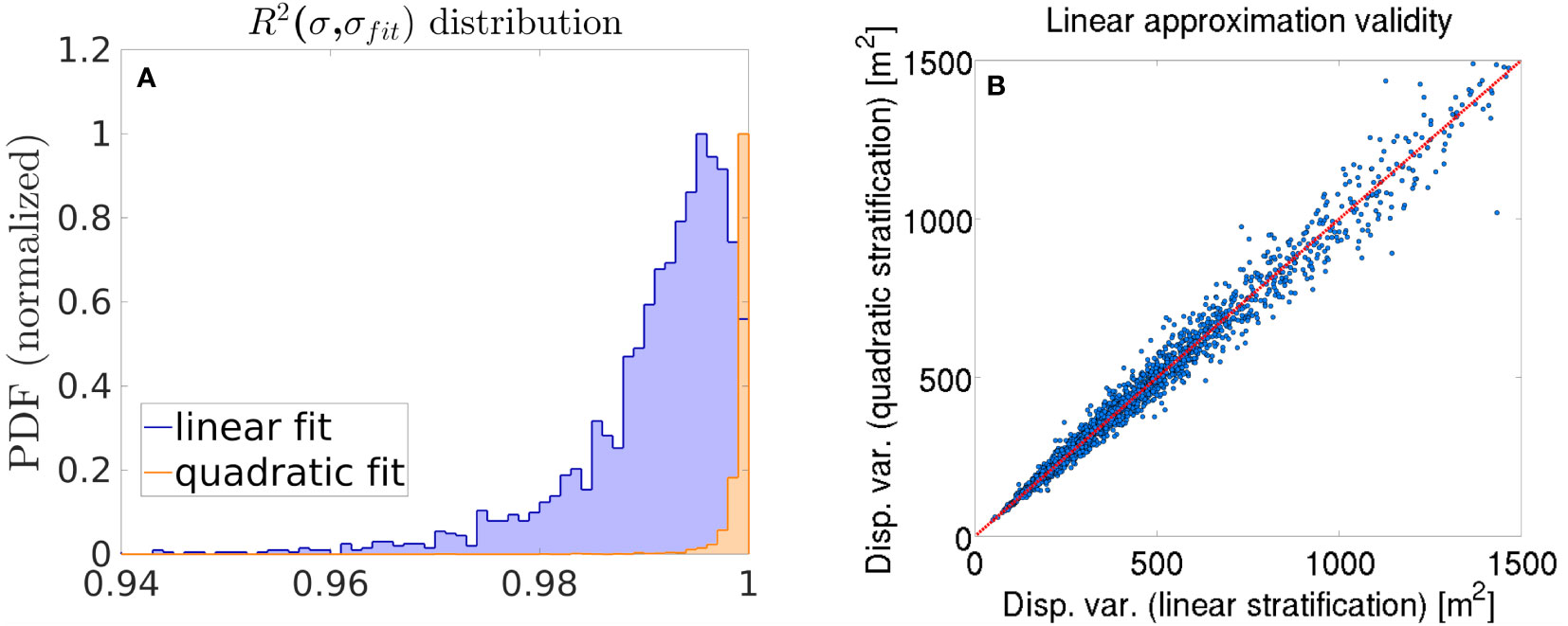
Figure 4 (A) Coefficient of determination of the fitted density profiles. The blue and orange distributions represent the linear and quadratic fits, respectively. (B) displacement variance computed using the quadratic density profile against that using the linear density profile.

For each time series, the final isopycnal displacements used in this work are computed following Hennon et al. (2014), using the γ value computed using a linear regression on σ_r(z) over the range spanned by the equivalent pressure p_e(t). An example of isopycnal displacement time series during the float drift is shown in Figure 5.

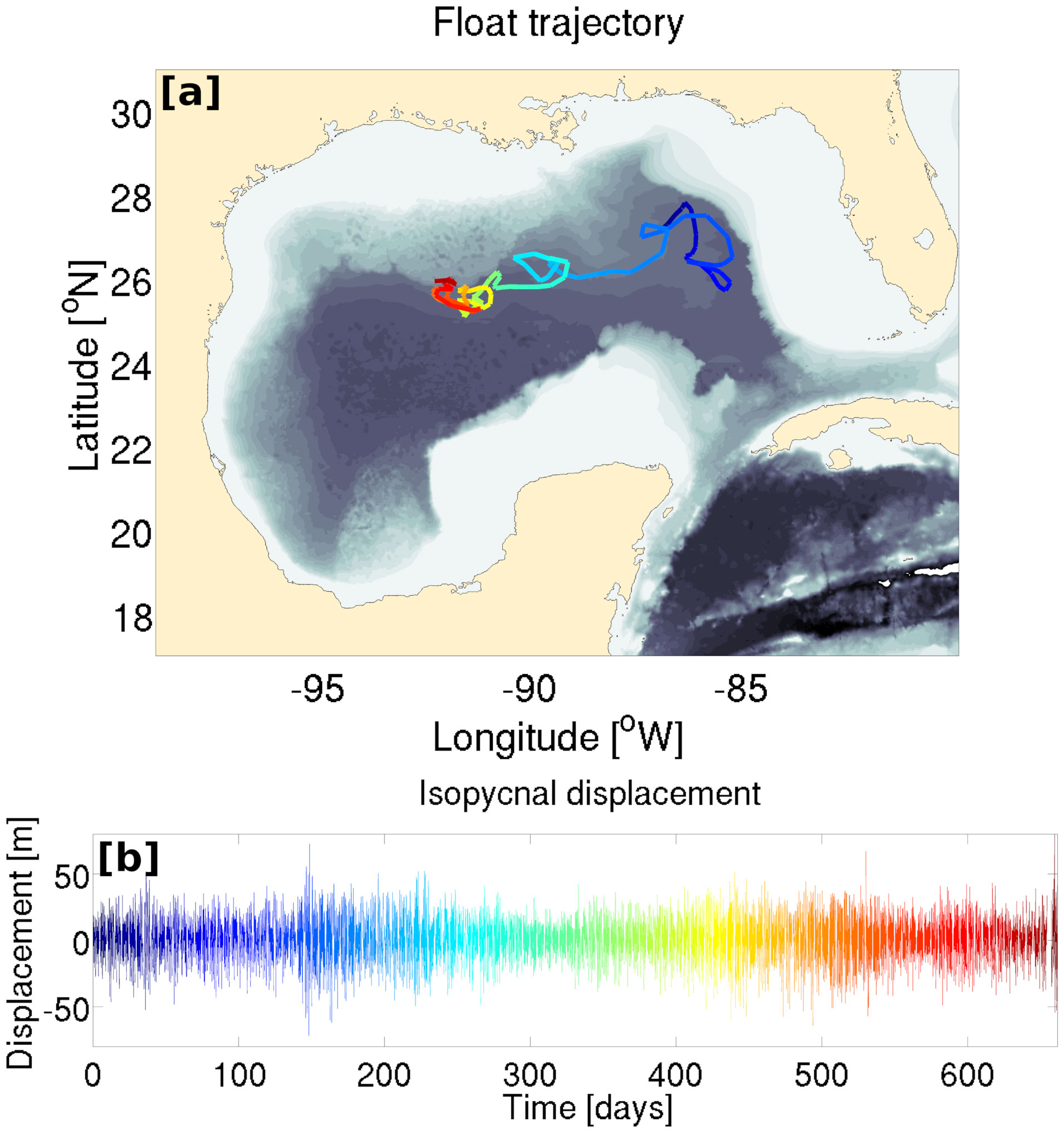
Figure 5 (A) Example of the trajectory of a drifting profiling float. Time is color-coded [time reference is shown in (B)]. (B) Reconstructed isopycnal displacement time series corresponding to the same float trajectory.

To ensure that, despite the good agreement between the observed density profiles and the linear fit, no bias is introduced for large isopycnal displacements, we computed the isopycnal displacement variance for each time series, using the linear and the quadratic fits as a reference profile. Displacement variance using the linear approximation is plotted against displacement variance using the quadratic approximation in Figure 4B. The symmetry of the scattering shows that the linear approximation does not introduce a bias in the displacement variance, even for larger displacement variances.

The power spectral density of isopycnal displacement (here after displacement variance spectrum) is defined as:

where ν is the frequency and τ is the record’s length (constant and equal to 5 days here). S(ν) represents the distribution of the signal’s energy across frequencies normalized by the record’s length. Note that the raw displacement variance spectrum does not represent the energy spectrum in the physical sense. To estimate the APE distribution across frequencies, we need to compute the variance spectrum from the BFS isopycnal displacements (since the squared BFS displacement is proportional to APE, the BFS displacement variance spectrum represents the distribution of APE across frequencies). Noting S_BFS the variance spectrum of the BFS displacements, the APE spectrum is:

To map the internal wave activity geographically, we averaged the variances of the time series on a 0.5° grid of the GoM. The location of each time series was chosen as the middle point between the two surfacings. Since the average float displacement during one drift phase is of 26 km $(\approx 1/4\mathbf{V}\mathbf{A}{\mathbf{R}}_{\text{NI}}={\displaystyle {\int }_{0.7f}^{1.3f}\mathbf{S}}d\nu ,\mathbf{V}\mathbf{A}{\mathbf{R}}_{CON}={\displaystyle {\int }_{3cpd}^{8cpd}\mathbf{S}d\nu }$

The 8 cpd value was chosen to be slightly smaller than the minimum buoyancy frequency found in the GoM dataset.

The Garett and Munk (GM) frequency spectra (Garrett and Munk, 1975; Cairns and Williams, 1976) were computed using J. Klymak’s Garrett and Munk internal wave spectra Matlab Toolbox (available online at https://jklymak.github.io/GarrettMunkMatlab/).

3 Results

The mean raw and BFS displacement spectra were computed for each time series and averaged for the whole GoM (Figure 6). The average inertial period in the GoM ranges between 24 and 29 hours, so each time series only lasts 4 to 5 inertial periods. The resulting lack of frequency resolution on the left-hand-side of the spectrum result in a wide and smooth peak between 0.7 and 1.3 cpd. Variability in the inertial frequency between the south and north of the surveyed area also participates in this smoothing of the near-inertial peak. Despite being more accurately resolved in the spectral analysis, signatures of the M2 and S2 tides are barely distinguishable, suggesting a negligible contribution of the semi-diurnal tide to the total variance. The Garrett and Munk frequency spectrum was computed using the dataset’s average buoyancy and Coriolis frequencies and is compared to the raw displacement spectrum in Figure 6A. On the low end of the continuum, between 2 and 6 cpd, the mean displacement spectrum’s slope is slightly flatter and exhibits a slightly lower energy level than the reference GM spectrum. At higher frequencies, between 6 cpd and the buoyancy frequency, the displacement spectrum coincides with the GM spectrum both in terms of slope and energy level. It should be pointed out that the frequency measured by the profiling floats slightly differs from the frequency that would be measured by a fixed point instrument. During the drift phase, the profiling floats can be considered as Lagrangian floats, as they drift along with the currents. Therefore, the frequency they measure is the intrinsic frequency of the internal wave, whithout the aliasing effects of the current that arise with moored instruments.

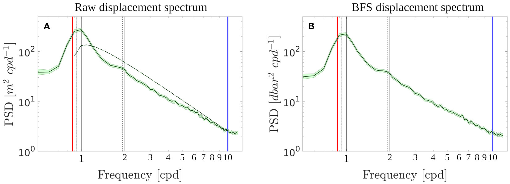
Figure 6 (A) Mean raw displacement variance spectrum for all time series. The Garrett and Munk spectrum corresponding to the average Coriolis and buoyancy frequency is plotted as a dashed-dotted line. The red and blue vertical lines represent the average Coriolis and buoyancy frequencies, respectively. The vertical black lines represent the O1, K1, M2 and S2 tidal frequencies. (B) Same as (A) for the BFS isopycnal displacements.

3.1 Geographical distribution

Spatial distribution of the mean total variance, computed by integrating the displacement spectrum over the whole frequency range between 0.7×f and the buoyancy frequency, is shown in Figure 7A. Magenta contours represent contours of the LC presence probability (0.1, 0.5, and 0.9) and are plotted to help locate the area of influence of the LC. A clear pattern emerges, with a large patch of high variance between the eastern Campeche Bank and the West Florida Shelf (87-83°W;22-25.5°N), in the LC region. Outside of this region, variance decreases northward and westward, except for sparse grid-points with increased variance along the Texas-Louisiana Shelf.

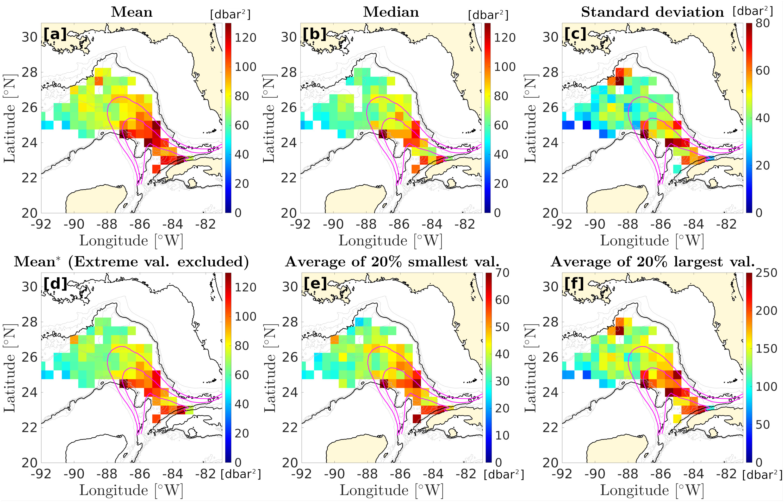
Figure 7 Maps of the displacement variance on a 0.5° grid. (A) shows the results using the average of all available data for each grid point; (B) shows the median; (C) shows the standard deviation; (D) shows the average excluding the 20% largest and smallest values; (E) shows the average of the 20% smallest values, and (F) the average of the 20% largest values. The magenta contours represent the Loop Current presence probability. The outtermost contour is 0.1, the middle contour is 0.5, and the southernmost contour is 0.9.

The geographical distribution of internal wave activity is key in this study, and the observations are not evenly distributed in the study area, with time series number per grid point varying between 10 and 64 (Figure 1). To make sure the average variance in each grid point is representative, we computed a series of different metrics to validate the statistics. At each grid-points, we also computed the median variance (Figure 7B), the standard deviation (Figure 7C), the average excluding the 20% smallest and 20%largest values (Figure 7D), the average of the 20% smallest variance samples (Figure 7E), and the average of the 20% largest variance samples (Figure 7F). Despite a larger standard deviation in the LC region, the increased displacement variance pattern detected in the mean variance map is clearly evident in all metrics, including when removing the extreme small values, extreme large values, or both. This pattern can thus not be attributed to a bias due to some outlier time series. Oppositely, the increased displacement variance off the Texas Louisiana Shelf, which is also associated with increased standard deviation, is absent from the median displacement variance map, as well as the mean displacement variance map excluding extreme values and the mean displacement variance map only taking into account the 20% smallest values. It is however evident in the map of the mean of the 20% largest variance. This pattern might therefore be attributable to a small number of time series exhibiting unusually large isopycnal displacements and is not representative of typical conditions at these locations.

The raw displacement and the BFS displacement variances were decomposed into the continuum and the near-inertial bands, as defined in section 2.2, and the maps are shown in Figure 8. In the continuum band (Figure 8A), the pattern of increased raw-displacement variance in the LC region is similar to that observed in the total variance map of Figure 7A. In the near-inertial band, increased raw-displacement variance is also observed in the LC region, except for a patch of low variance north of Cuba. As discussed in section 2.2, for a given energy, raw-displacement variance depends on local stratification. To allow for direct comparison between different geographical locations with different stratification properties, we computed maps of the BFS displacement variance, which is proportional to APE (Figures 8C, D). The patterns of increased variance observed both in the continuum and the near-inertial bands become even more evident when looking at the BFS displacements. In the continuum and in the near-inertial band, BFS displacement variance is 4 to 5 times larger in the LC region than in the rest of the basin, while the patterns remain similar to the raw-displacement variance spatial structure.

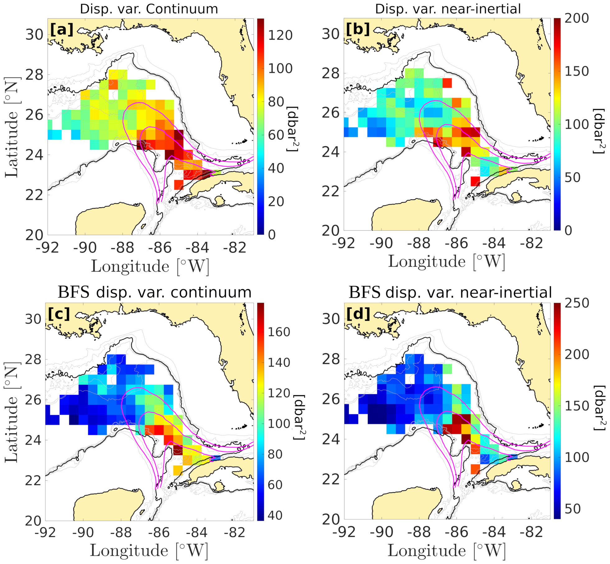
Figure 8 Maps of the displacement variance. (A) Raw displacement variance in the continuum band ([3—8]cpd). (B) Same as (A) in the near inertial band ([0.7f—1.3f]). (C) buoyancy frequency-scaled (BFS) displacement variance in the continuum band. (D) Same as (C) in the near-inertial band. The magenta contours represent the Loop Current presence probability. The outtermost contour is 0.1, the middle contour is 0.5, and the southernmost contour is 0.9.

3.2 Driving mechanisms

To understand the reasons for the increase of APE in the region of influence of the LC, we selected a subset of the data in that area to perform a sensitivity study of parameters that might be relevant for internal wave energy: deep current velocity (computed from float displacements at the parking depth), bottom roughness, float altitude above the seafloor, wind speed, wind intermittency, and sea surface height (SSH) which is a proxy for the presence or absence of the LC above the float at the time of measurement. The position of the selected profiles and time series is shown in Figure 9. The blue dots represent observations measured below the LC, while the red dots represent observations measured outside of the LC.

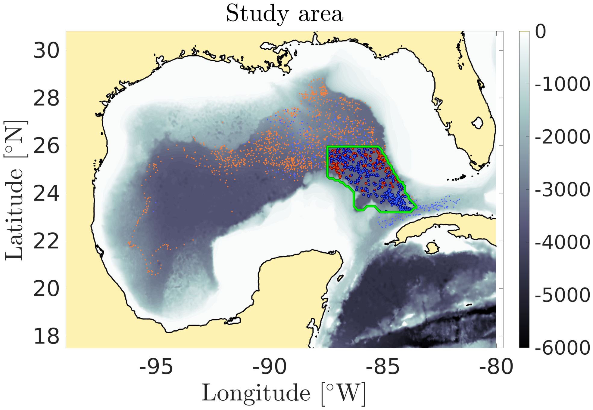
Figure 9 Map of the sensitivity study area (green contour). The blue and red dots represent observations under the Loop Current (LC) and outside of the LC, respectively.

For each parameter, the data were sorted into subsets, and the BFS variance spectra were averaged for each subset, as well as the continuum and near-inertial bands variances. 90% confidence intervals were computed in each subset using the bootstrap method.

The LC has a strong signature in sea surface height (SSH), so that the latter can be used to infer the LC’s presence. The LC and LC rings boundaries have traditionally been defined as the 17 cm sea level anomaly isopleth (Leben and Born, 1993; Leben, 2005). Using AVISO ADT, we found that, on average, the LC edge (defined as the isopleth linking the Yucatan Channel and the Florida Strait with the smallest SSH value) coincides to the 50 cm SSH isopleth, consistent with Meunier et al. (2018). Below this 50 cm SSH threshold, decreasing SSH coincides with increasing the distance from the LC. Beyond 50 cm, increasing SSH coincides with getting closer to the LC’s core. The raw and BFS displacement spectra for all SSH ranges are shown in Figures 10A, B, respectively, and 2D maps of power spectral densities in the SSH-frequency space are shown in Figures 10C, D. At all frequencies below 9 cpd, raw displacement power spectral density increases with decreasing SSH (Figures 10A, C). At higher frequencies, the tendency reverses as low-SSH spectral slopes increase while high-SSH spectral slopes remain constant. This steepness increase in the spectra occurs as the frequency exceeds the buoyancy frequency, which increases with increasing SSH (Figure 11B). The BFS displacement spectra (Figures 10B, D) exhibit opposite results to the raw displacement spectra: at all frequencies, power spectral density increases with increasing SSH, meaning that there is more APE in the LC than outside of it, and that APE gradually increases towards the very core of the LC. The increase of the BFS displacement variance with SSH is evidenced in Figure 12 for both the continuum and the near-inertial band. The opposite results between raw displacement and BFS displacement spectra can be explained by the relationship between SSH and buoyancy frequency: since the buoyancy frequency increases with increasing SSH, the BFS variance is proportional to the squared buoyancy frequency, a lower raw displacement variance can result in a larger BFS displacement variance if the water column is more stratified (more energy is required to raise isopycnal in a strongly stratified medium). Figure 11A shows a map of the mean buoyancy frequency computed from the profiling float data. The LC region has an increased stratification compared to the rest of the eastern GoM. Within the LC region, Figure 11B shows a scatter plot of buoyancy frequency against in situ steric height. It shows that stratification increases with increasing SSH, so that buoyancy frequency increases in the presence of the LC, and decreases outside of it. The decrease in raw-displacement variance under the LC while APE is actually increased results from this larger stratification.

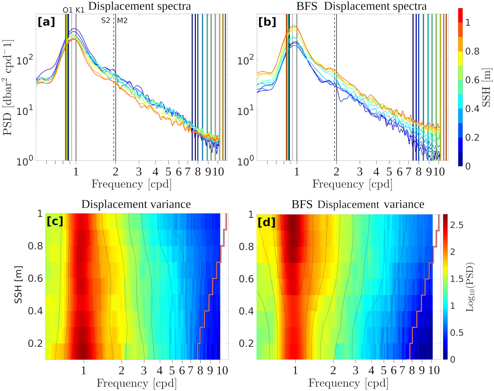
Figure 10 (A) Raw displacement variance spectra for 10 different ranges of sea surface height (SSH). SSH is color coded. The black vertical lines represent the O1, K1, M2 and S2 tidal frequencies (from left to right). The colored lines on the left-hand side (low frequencies) represent the mean Coriolis frequency for each SSH range. The colored lines on the right-hand side (high frequencies) represent the mean buoyancy frequencies for each SSH range. (B) Same as (A) for the buoyancy frequency-scaled (BFS) isopycnal displacements. (C) Contour plot of the power spectral density of the raw isopycnal displacements against frequency and SSH. The mean buoyancy frequency for each SSH range is shown as a light red line. (D) Same as (C) for the BFS isopycnal displacements.

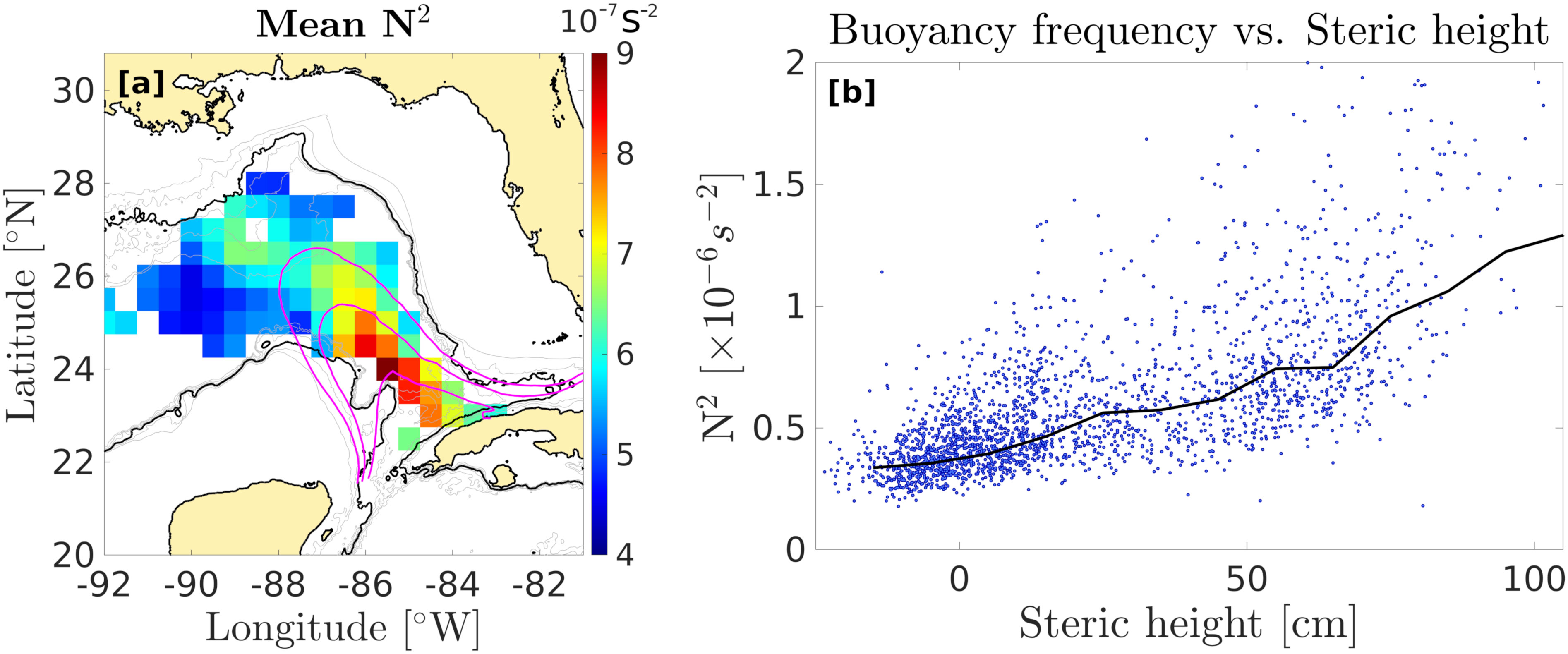
Figure 11 (A) Map of the mean squared buoyancy frequency at the parking depth on the 0.5^◦ grid. (B) Squared buoyancy frequency against steric height for all available profiles. The blue dots represent raw data, while the black line is averaged over ranges of 5 cm.

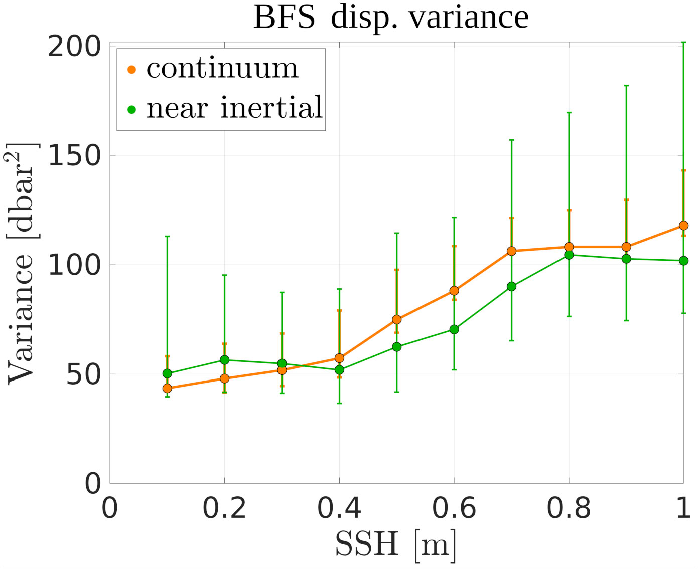
Figure 12 buoyancy frequency-scaled (BFS) variance against SSH. The green line and dots represent the near-inertial band, while the orange ones stand for the continuum.

As a deep flow encounters topographic irregularities, vertical velocities are generated and deflect isopycnals, resulting in the propagation of internal waves (Bell, 1975; Garrett and Munk, 1979; Nikurashin and Ferrari, 2010). The importance of bottom roughness was demonstrated by Hennon et al. (2014) using a similar float dataset. Following Hennon et al. (2014), bottom roughness is defined as the Gaussian-weighted standard deviation of bottom depth with a length scale L:

where x is the position vector where roughness is estimated, x_i of all other grid points, D is water depth, and w is a Gaussian weight. Here, the roughness was computed using a 50 km length scale [mean 1st Rossby radius in the GoM; Meunier et al. (2018)]. The BFS displacement spectra averaged over a series of roughness ranges and the corresponding variances in the continuum and near-inertial bands are shown in Figures 13A, E, respectively. At all frequencies, increased roughness is associated with increased power spectral density, so that both the continuum and the near-inertial band variances grow with roughness. Note that high roughness ranges have slightly noisier spectra because of reduced sample numbers.

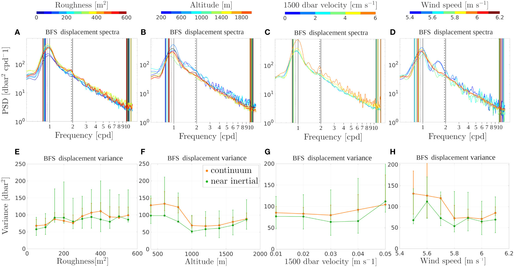
Figure 13 (A) buoyancy frequency-scaled (BFS) displacement variance spectra for 12 different ranges of bottom roughness. Roughness is color coded. The black vertical lines represent the O1, K1, M2 and S2 tidal frequencies (from left to right). The colored lines on the left-hand side (low frequencies) represent the mean Coriolis frequency for each range. The colored lines on the right-hand side (high frequencies) represent the mean buoyancy frequencies for each range. (B) Same as (A) for float altitude. (C) Same as (A) for the 1500 dbar velocity. (D) Same as (A) for wind speed. (E) BFS variance against bottom roughness. The green line and dots represent the near-inertial band, while the orange ones represent the continuum. (F) Same as (E) for the float altitude. (G) Same as (E) for the 1500 dbar velocity. (H) Same as (E) for the wind speed.

The impact of deep velocity was also investigated. Because no direct measurements right above the topography are available, we used the profiling float displacements at the parking depth (1500 dbar). Recent moored ADCP observations by Tenreiro et al. (2018) showed that, while the top 900 dbar of the GoM were strongly baroclinic, the deep layer between 1200 and 3500 dbar could be considered as nearly homogeneous. For that reason, we stress that the 1500 dbar velocity (the only available with ths dataset) might be a solid proxy for the bottom velocity. A map of the gridded mean velocity field, computed from the float displacements, is shown in Figure 14. Contours of BFS displacement variance, as well as contours of LC presence probability, are overlaid. In the area of increased variance, velocity vectors strictly follow the continental slope around the Campeche Bank and the flow field is dominated by a cyclonic circulation in deep water. The BFS displacement spectra sorted by velocity magnitude are shown in Figure 13C and the variance is plotted against the 1500 dbar velocity for the continuum and near-inertial bands in Figure 13G. Increasing the velocity does not seem to affect the spectra between 1 and 3 cm s⁻¹. Beyond a threshold value, variance increases. Note that this threshold value is smaller in the continuum (3 cm s⁻¹) than in the near-inertial band (4 cm s⁻¹). Note that there is increased noise in the averaged spectra for high-velocity ranges and that the variance confidence intervals are large, so that any conclusion is subject to caution.

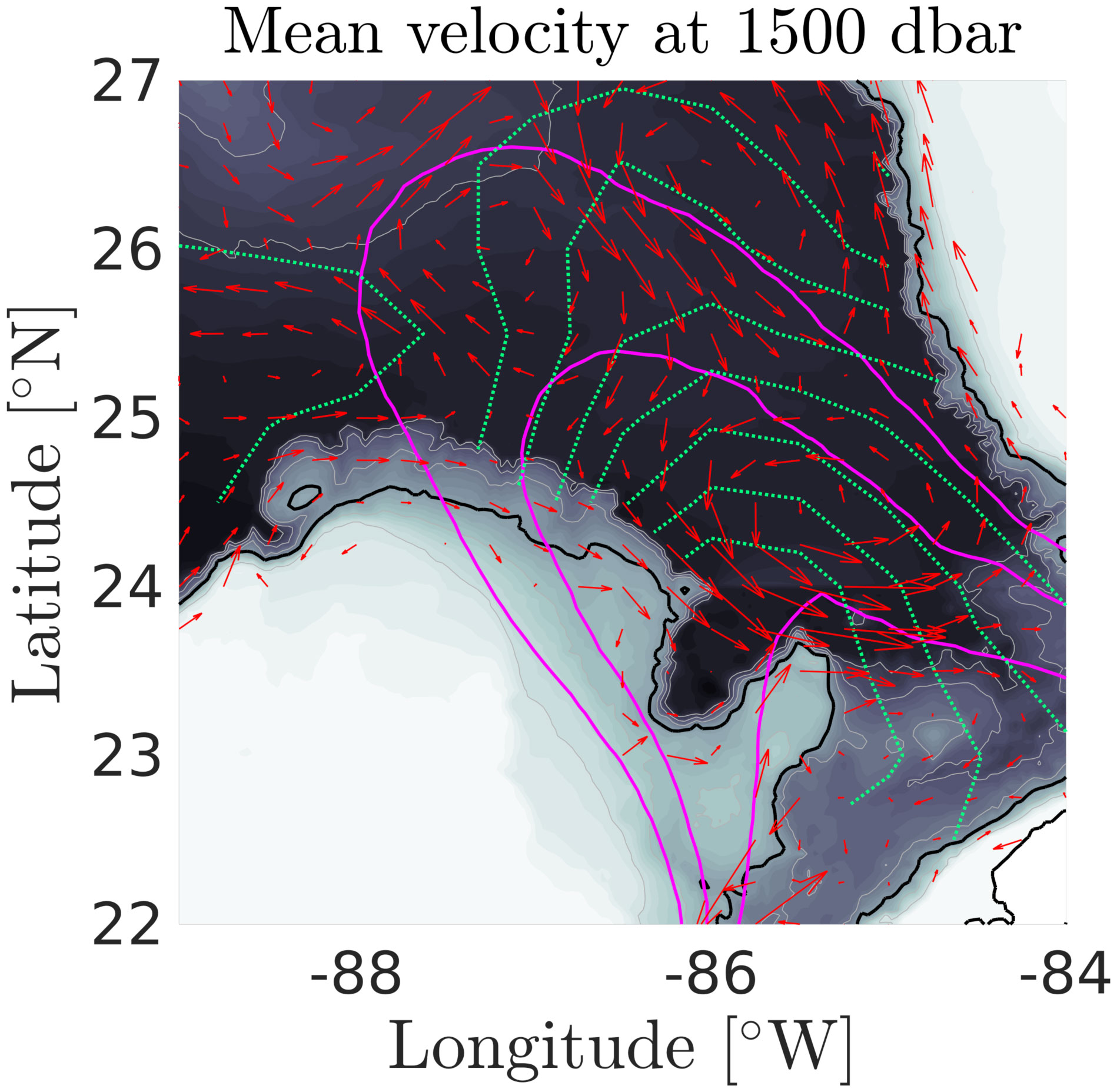
Figure 14 Gridded mean velocity at the parking depth (≈1500 dbar) inferred from float displacements (red arrows). The green contour represent the mean gridded buoyancy frequency-scaled (BFS) displacement variance. The magenta contours represent the Loop Current presence probability (0.1, 0.5, and 0.9). Topography is represented as shades of gray, and the black contour shows the 1500 dbar isobath.

The float altitude is also a relevant parameter for internal wave variance. When internal waves are generated by a deep current flowing over rough topography, isopycnal displacement is expected to be maximum close to the topography. The BFS displacement spectra averaged by float altitude ranges are shown in Figure 13C and the variances for the continuum and near-inertial ranges are plotted against altitude in Figure 13G. Floats with low altitudes (<600 m) exhibit larger variance, especially in the continuum frequency range. On the other hand, beyond 1000 m, altitude does not seem to impact the spectrum, and the variance increases gently with increasing altitude (Figure 13B). This increase of variance with altitude at all frequencies may be related to the fact that the LC presence probability (which was shown to increase variance) is higher in deep water.

To test for the possible impact of the surface wind on the increase in near-inertial variance, the dataset was sorted according to the local instantaneous wind speed and wind intermittency (running variance of wind speed over a 48 hours window; not shown). The wind product used is Copernicus Global Ocean Hourly Sea Surface Wind and Stress from Scatterometer and Model. The data is distributed on a 0.125° grid. The BFS displacement variance spectra are shown in Figure 13D. The spectra for weaker wind ranges exhibit an increased noise level because of a smaller sample size. In the near inertial band, where we would expect to see an impact of increasing wind speed (or wind intermittency), if any, no trend exists in the variance/wind speed relationship. Note that there exist a time lag between the generation of inertial oscillations by the wind at the sea surface and their downward propagation to such depth. Observations in the LC by Pallàs-Sanz et al. (2016a) show group speeds of about 70 m/day in the top 750 m. However, they also highlighted the presence of a critical layer near 500 m, beyond which the downward propagation of near-inertial energy might drastically change. Estimating a rigorous time lage between surface wind events and near-inertial waves at 1500 dbar therefore seems hazardous, and our results regarding the impact of wind on the observed internal wave activity must be interpreted cautiously.

4 Discussion and conclusion

Using profiling float data, including hourly along-drift sampling of temperature and salinity, we have explored the geography of internal wave activity in the eastern GoM at 1500 dbar. Both the raw isopycnal displacements and the BFS isopycnal displacements, whose variance is proportional to APE, have been considered. For each variable, the variances were computed both for the continuum and the near-inertial bands.

For both frequency ranges, we found a clear pattern of increased variance in the LC region, between the eastern Campeche Bank and the southern tip of the West-Florida Shelf. This pattern was observed for the raw displacement variance and was particularly striking for the APE (BFS displacement variance), which is on average 4 to 5 times larger in the LC region than in the north and west of the basin. However, we noted that, in a thin band along the northern Cuban Shelf, at the very base of the LC, internal wave activity is only increased in the continuum, and no anomalous signal is found in the near-inertial band.

We investigated the possible physical processes controlling this geographical distribution by isolating the time series within the LC region and sorting them according to a series of relevant variables, including bottom roughness, 1500 dbar current velocity, float altitude, wind speed and intermittency, as well as the local SSH, which is a proxy for the position of the float relative to the LC.

In the restricted LC influence region, rougher bottom, faster deep currents and lower float altitude are all associated with increased APE, both in the continuum and near inertial band. An increase in internal wave energy near the bottom as fast currents encounter steep topography is an expected result [e.g. Bell (1975)] and was previously demonstrated using Argo floats by Hennon et al. (2014). As the current encounters a topographic obstacle, an upward momentum flux is generated, which locally distorts isopycnals and sets up wave-motion (Bell, 1975). Recently, Clément et al. (2016) observed the systematic generation of internal waves as mesoscale eddies interact with the rough topography of the Bahamas continental slope using moored ADCPs. Their study confirmed that these topographically-generated internal waves were associated with increased diapycnal mixing. They also showed that the eddy’s flow-topography interactions generated more energy in the continuum than in the near-inertial frequency band. In our case, the increase of APE with increasing bottom roughness and deep velocity along with a decrease in float altitude, seems to be consistent with topographic generation. However, in most of the LC region, APE is also increased in the near inertial band. An increase of the continuum energy without a coincident increase in the near-inertial band, is however found in a narrow band along the North shore of Cuba, just east of the Yucatan Channel (Figure 8).

As the LC is an evolving structure, disturbed by large propagating meanders (Donohue et al., 2016a,b) and eventually changing from an extended to a retracted mode as rings are shed (Leben, 2005), we focused on the impact of the presence or absence of the LC above the floats inside the increased variance region. This was achieved by sorting the time series by the local SSH during sampling. The LC front is identified using the 50 cm SSH contour, and larger (smaller) values coincide with floats located further inside (outside) of the LC. In the region where raw displacement variance and APE are increased on average, we found that the position of the floats relative to the LC had a strong impact. Between SSH of ≈10 to 40 cm (that is, clearly outside of the LC’s influence), APE is low and constant. As SSH increases from ≈40 to ≈80 cm (that is between the LC front and its core), variance increases to reach a plateau at higher SSH values, where it is about twice as high as outside of the LC. This pattern was observed at all frequencies.

The fact that the geographical distribution of increased APE (and raw displacement variance) coincides with the region of high probability of presence of the LC, and that in that given region, the presence (absence) of the LC is correlated with an increase (decrease) of APE suggests a strong control of the LC over the internal wave activity in the eastern GoM.

It is important to remember that the LC, as defined here (which is the most common definition) is not only a fast current associated with a sharp front, but also includes a large pool of light water with closed isopleths of SSH near its core, associated with an anticyclonic circulation (think of it as a large warm-core anticyclonic eddy trapped between a meandering front and the south-east corner of the basin) (Leben, 2005; Lugo-Fernández et al., 2016).

The amplification and trapping of near-inertial waves at the base of negative vorticity structures, such as fronts and anticyclonic eddies, is a known phenomenon, so that it may seem a natural candidate to explain the observed increased internal-wave activity under the anticyclonic core of the LC. Kunze (1985) showed that the effective inertial frequency for a near-inertial wave propagating in a mesoscale flow field was modulated by the local relative vorticity. Considering this modulation and deriving a modified dispersion relation, he showed that waves with frequencies between the effective inertial frequency and the planetary inertial frequency could not propagate away from negative vorticity regions. This effect tends to accumulate near-inertial energy in zones of anticyclonic vorticity. Similar conclusions were obtained by Danioux et al. (2015) using alternative arguments. As relative vorticity approaches zero at the base of an anticyclonic eddy, near-inertial waves are expected to remain trapped in a critical layer below the eddy. Such downward and inward propagation of near-inertial waves within warm-core rings was described in detail using a primitive equation numerical model by Lee and Niiler (1998). This phenomenon was also repeatedly observed in situ (Kunze et al., 1995; Joyce et al., 2013).

Recently, Pallàs-Sanz et al. (2016b) observed the downward propagation of near-inertial waves in the LC after the passage of two hurricanes, using a mooring array in the eastern GoM equipped with current meters and ADCPs. However, they showed a concentration of near-inertial wave activity around 1000 m, in what seems like a critical layer at the base of the anticyclonic circulation of the LC. Despite this clear depth-localized energy increase, Pallàs-Sanz et al. (2016b) also shows remnants of near-inertial waves propagating down to 1500 m (see their Figure 6).

In our case, the profiling floats drift well below the depth of this supposed critical layer so that near inertial waves generated by the wind at the surface and propagating downward through this so-called inertial chimney phenomenon (Lee and Niiler, 1998) should not reach the depth of the floats as the critical layer is expected to act like a shield. Furthermore, we observed that the mean circulation below the southeast LC was cyclonic (Figure 14), in agreement with previous RAFOS floats observations (Pérez-Brunius et al., 2018), so one should rather expect near-inertial waves to be repelled and energy to be reduced (Lee and Niiler, 1998; Danioux et al., 2015).

As of now, it thus seems difficult to draw any definitive conclusion regarding the reasons for the increased internal wave activity under the LC. Similar to the high internal waves modes generated through the interaction between current and topography, all sorts of low frequency waves (lee and near inertial waves) propagating upward can also be observed in the ocean (Waterhouse et al., 2022). Near-inertial internal waves can be excited by steady or slowly evolving, low-frequency geostrophic flow impinging on seafloor topography, which can develop into near-inertial waves – through a resonant feedback – that produces near-inertial waves with velocity amplitudes similar to those of the overlying geostrophic flow (Nikurashin and Ferrari, 2010). This process is initiated through classic lee-wave generation and deposits momentum nonuniformly into the overlying fluid while propagating. These lee waves induce spatially varying nearinertial oscillations. In turn, these oscillations alter near-bottom velocities and hence add time dependence to the lee-wave generation at the inertial frequency. For sufficient geostrophic flow and topographic amplitude, this feedback is strong enough that the overlying flow can saturate in timescales of less than a few days, making the energy transfer particularly efficient.

While this study does not find direct evidence of increased diapycnal mixing in the LC region, the intense internal wave activity – compared to the rest of the central and eastern basin – suggests that part of the mixing necessary for the warming of the bottom layer NADW may occur in this area. The link between internal wave activity and diapycnal mixing was clearly demonstrated in a number of studies over the past four decades [e.g. Garrett and Munk (1975); Gregg and Briscoe (1979); Polzin et al. (1995); Müller and Briscoe (2000); Whalen et al. (2020)]. While vertical profiles of temperature and salinity, including those obtained from profiling floats can provide estimates of turbulent diffusivity by using fine-scale strain parameterizations (Polzin et al., 1995; MacKinnon et al., 2009; Whalen et al., 2012; Whalen et al., 2015), such methods, based on local meter to 10 meter-scale deviations of the buoyancy frequency from its mean value (Whalen et al., 2015), are only accurate with high resolution measurements or in well-stratified water columns. In the GoM, the NADW, in which our observations were sampled, is a particularly homogeneous water mass. Because of the coarse resolution of the Seabird SBE 41 CTD (relative to the weak stratification of the water mass), strain is essentially dominated by noise at 1-10 meters-scale (see Figures 2C, D), so that our estimates of turbulent diffusivity would essentially be dominated by noise.

Contrary to Molodtsov et al. (submitted manuscript), who provided direct estimates of diapycnal mixing from microstructure measurements along the western GoM’s continental slope and a quantitative description of the possible sources of mixing for the NADW and the AAIW, our conclusions regarding mixing of the GoM’s bottom layers remain speculative. It is however puzzling to observe such an increased internal wave activity in the LC a few hundreds meters above the depth of the Yucatan Sill. This surprising geographical distribution of the internal wave activity under the LC and in the vicinity of the Yucatan Channel is however suggestive of an alternative source of ventilation for the GoM’s NADW layer, and further experiments, including direct microstructure measurements are needed to confirm the potential role of the LC in ventilating the deep GoM.

Data availability statement

Publicly available datasets were analyzed in this study. This data can be found here: https://co.ifremer.fr/co-dataSelection/?theme=argo.

Author contributions

TM: Conceptualization, Data curation, Formal Analysis, Investigation, Methodology, Software, Validation, Visualization, Writing – original draft, Writing – review & editing. AL: Conceptualization, Formal Analysis, Investigation, Writing – original draft, Writing – review & editing. SM: Writing – review & editing. AB: Funding acquisition, Project administration, Writing – review & editing. HF: Project administration, Resources, Writing – review & editing. PR: Resources, Writing – review & editing.

Funding

The author(s) declare financial support was received for the research, authorship, and/or publication of this article. This work is part of the LC-floats and UGOS3 projects, funded by the US National Academy of Sciences through the Understanding Gulf Ocean Systems grants to the Woods Hole Oceanographic Institution 2000010488 and 200013145.

Acknowledgments

TM is grateful to John Toole at WHOI for his invaluable advice and comments during the analysis of the profiling floats data.

Conflict of interest

The authors declare that the research was conducted in the absence of any commercial or financial relationships that could be construed as a potential conflict of interest.

Publisher’s note

All claims expressed in this article are solely those of the authors and do not necessarily represent those of their affiliated organizations, or those of the publisher, the editors and the reviewers. Any product that may be evaluated in this article, or claim that may be made by its manufacturer, is not guaranteed or endorsed by the publisher.

References

Alford M. H., MacKinnon J. A., Simmons H. L., Nash J. D. (2016). Near-inertial internal gravity waves in the ocean. Annu. Rev. Mar. Sci. 8, 95–123. doi: 10.1146/annurev-marine-010814-015746
Amon R. M., Ochoa J., Candela J., Herzka S. Z., Pérez-Brunius P., Sheinbaum J., et al. (2023). Ventilation of the deep Gulf of Mexico and potential insights to the atlantic meridional overturning circulation. Sci. Adv. 9, eade1685. doi: 10.1126/sciadv.ade1685
Austin J., George B. (1955). Some recent oceanographic surveys of the Gulf of Mexico. Transact. Am. Geophys. Union 36, 885–892. doi: 10.1029/TR036i005p00885
Bell J. T.H. (1975). Topographically generated internal waves in the open ocean. J. Geophys. Res. 80 (3), 320–327. doi: 10.1029/JC080i003p00320
Cairns J. L., Williams G. O. (1976). Internal wave observations from a midwater float, 2. J. Geophys. Res. 81 (12), 1943–1950. doi: 10.1029/JC081i012p01943
Chapman P., DiMarco S. F., Key R. M., Previti C., Yvon-Lewis S. (2018). Age constraints on Gulf of Mexico deep water ventilation as determined by 14c measurements. Radiocarbon 60, 75–90. doi: 10.1017/RDC.2017.80
Clément L., Frajka-Williams E., Sheen K. L., Brearley J. A., Garabato A. C. N. (2016). Generation of internal waves by eddies impinging on the western boundary of the North Atlantic. J. Phys. Oceanogr. 46, 1067–1079. doi: 10.1175/JPO-D-14-0241.1
Danioux E., Vanneste J., Bühler O. (2015). On the concentration of near-inertial waves in anticyclones. J. Fluid Mechanics 773, R2. doi: 10.1017/jfm.2015.252
Donohue K. A., Watts D. R., Hamilton P., Leben R., Kennelly M. (2016a). Loop Current Eddy formation and baroclinic instability. Dyn. Atmos. Oceans 76, 195–216. doi: 10.1016/j.dynatmoce.2016.01.004
Donohue K. A., Watts D. R., Hamilton P., Leben R., Kennelly M., Lugo-Fernández A. (2016b). Gulf of Mexico Loop Current path variability. Dyn. Atmos. Oceans 76, 174–194. doi: 10.1016/j.dynatmoce.2015.12.003
Garrett C., Munk W. (1975). Space-time scales of internal waves: A progress report. J. Geophys. Res. 80 (3), 291–297. doi: 10.1029/JC080i003p00291
Garrett C., Munk W. (1979). Internal waves in the ocean. Annu. Rev. Fluid Mechanics 11, 339–369. doi: 10.1146/annurev.fl.11.010179.002011
Gregg M. C. (1989). Scaling turbulent dissipation in the thermocline. J. Geophys. Res.: Oceans 94, 9686–9698. doi: 10.1029/JC094iC07p09686
Gregg M., Briscoe M. G. (1979). Internal waves, finestructure, microstructure, and mixing in the ocean. Rev. Geophys. 17, 1524–1548. doi: 10.1029/RG017i007p01524
Hamilton P., Leben R., Bower A., Furey H., Pérez-Brunius P. (2018). Hydrography of the Gulf of Mexico using autonomous floats. J. Phys. Oceanogr. 48, 773–794. doi: 10.1175/JPO-D-17-0205.1
Hennon T. D., Riser S. C., Alford M. H. (2014). Observations of internal gravity waves by argo floats. J. Phys. Oceanogr. 44, 2370–2386. doi: 10.1175/JPO-D-13-0222.1
Jing Z., Chang P., DiMarco S. F., Wu L. (2015). Role of near-inertial internal waves in subthermocline diapycnal mixing in the Northern Gulf of Mexico. J. Phys. Oceanogr. 45, 3137–3154. doi: 10.1175/JPO-D-14-0227.1
Jing Z., Chang P., DiMarco S. F., Wu L. (2018). Observed energy exchange between low-frequency flows and internal waves in the Gulf of Mexico. J. Phys. Oceanogr. 48, 995–1008. doi: 10.1175/JPO-D-17-0263.1
Joyce T. M., Toole J. M., Klein P., Thomas L. N. (2013). A near-inertial mode observed within a Gulf Stream warm-core ring. J. Geophys. Res. (Oceans) 118, 1797–1806. doi: 10.1002/jgrc.20141
Kunze E. (1985). Near-inertial wave propagation in geostrophic shear. J. Phys. Oceanogr. 15, 544–565. doi: 10.1175/1520-0485(1985)015⟨0544:NIWPIG⟩2.0.CO;2
Kunze E., Firing E., Hummon J. M., Chereskin T. K., Thurnherr A. M. (2006). Global abyssal mixing inferred from lowered ADCP shear and CTD strain profiles. J. Phys. Oceanogr. 36, 1553. doi: 10.1175/JPO2926.1
Kunze E., Schmitt R. W., Toole J. M. (1995). The energy balance in a warm-core ring’s near-inertial critical layer. J. Phys. Oceanogr. 25, 942–957. doi: 10.1175/1520-0485(1995)025<0942:TEBIAW>2.0.CO;2
Leben R. R. (2005). Altimeter-derived loop current metrics. Washington DC Am. Geophys. Union Geophys. Monograph Ser. 161, 181–201. doi: 10.1029/161GM15
Leben R. R., Born G. H. (1993). Tracking Loop Current eddies with satellite altimetry. Adv. Space Res. 13, 325–333. doi: 10.1016/0273-1177(93)90235-4
Le Boyer A., Alford M. H. (2021). Variability and sources of the internal wave continuum examined from global moored velocity records. J. Phys. Oceanogr. 51, 2807–2823. doi: 10.1175/JPO-D-20-0155.1
Lee D.-K., Niiler P. P. (1998). The inertial chimney: The near-inertial energy drainage from the ocean surface to the deep layer. J. Geophys. Res. 103 (C4), 7579–7591. doi: 10.1029/97JC03200
Lugo-Fernández A., Leben R. R., Hall C. A. (2016). Kinematic metrics of the Loop Current in the Gulf of Mexico from satellite altimetry. Dyn. Atmos. Oceans 76, 268–282. doi: 10.1016/j.dynatmoce.2016.01.002
MacKinnon J., Alford M., Bouruet-Aubertot P., Bindoff N., Elipot S., Gille S., et al. (2009). “Using global arrays to investigate internal-waves and mixing,” in Proceedings of the OceanObs09 Conference: Sustained Ocean Observations and Information for Society, Venice, Italy, Vol. 2.
McComas C. H., Bretherton F. P. (1977). Resonant interaction of oceanic internal waves. J. Geophys. Res. 82 (9), 1397–1412. doi: 10.1029/JC082i009p01397
Meunier T., Pallás-Sanz E., Tenreiro M., Portela E., Ochoa J. L., Ruíz-Angulo A., et al. (2018). The vertical structure of a loop current eddy. J. Geophys. Res.: Oceans 123, 6070–6090. doi: 10.1029/2018JC013801
Molodtsov S., Anis A., Amon R. M. W., Perez-Brunius P., Sheinbaum J., Candela J., et al. (submitted manuscript). Enhanced mixing along the continental slope in the western Gulf of Mexico observed from microstructure glider measurements.
Müller P., Briscoe M. (2000). Diapycnal mixing and internal waves. Oceanography 13, 98–103. doi: 10.5670/oceanog.2000.40
Nikurashin M., Ferrari R. (2010). Radiation and dissipation of internal waves generated by geostrophic motions impinging on small-scale topography: theory. J. Phys. Oceanogr. 40, 1055–1074. doi: 10.1175/2009JPO4199.1
Nowlin W., McLellan H. (1967). A characterization of Gulf of Mexico waters in winter. J. Mar. Res. 25, 29.
Ochoa J., Ferreira-Bartrina V., Candela J., Sheinbaum J., López M., Pérez-Brunius P., et al. (2021). Deep-water warming in the Gulf of Mexico from 2003 to 2019. J. Phys. Oceanogr. 51, 1021–1035. doi: 10.1175/JPO-D-19-0295.1
Oey J. L. Y., Ezer T., Lee H. C. (2005). Loop current, rings and related circulation in the Gulf of Mexico: a review of numerical models and future challenges. Washington DC Am. Geophys. Union Geophys. Monograph Ser. 161, 31–56. doi: 10.1029/161GM04
Pallàs-Sanz E., Candela J., Sheinbaum J., Ochoa J. (2016a). Mooring observations of the nearinertial wave wake of Hurricane Ida, (2009). Dyn. Atmos. Oceans 76, 325–344. doi: 10.1016/j.dynatmoce.2016.05.003
Pallàs-Sanz E., Candela J., Sheinbaum J., Ochoa J., Jouanno J. (2016b). Trapping of the nearinertial wave wakes of two consecutive hurricanes in the Loop Current. J. Geophys. Res. (Oceans) 121, 7431–7454. doi: 10.1002/2015JC011592
Pérez-Brunius P., Furey H., Bower A., Hamilton P., Candela J., Garc´ıa-Carrillo P., et al. (2018). Dominant circulation patterns of the deep Gulf of Mexico. J. Phys. Oceanogr. 48, 511–529. doi: 10.1175/JPO-D-17-0140.1
Polzin K. L., Lvov Y. V. (2011). Toward regional characterizations of the oceanic internal wavefield. Rev. Geophys. 49, RG4003. doi: 10.1029/2010RG000329
Polzin K. L., Naveira Garabato A. C., Huussen T. N., Sloyan B. M., Waterman S. (2014). Finescale parameterizations of turbulent dissipation. J. Geophys. Res.: Oceans 119, 1383–1419. doi: 10.1002/2013JC008979
Polzin K. L., Toole J. M., Schmitt R. W. (1995). Finescale parameterizations of turbulent dissipation. J. Phys. Oceanogr. 25, 306–328. doi: 10.1175/1520-0485(1995)025⟨0306:FPOTD⟩2.0.CO;2
Portela E., Tenreiro M., Pallàs-Sanz E., Meunier T., Ruiz-Angulo A., Sosa-Gutiérrez R., et al. (2018). Hydrography of the central and western Gulf of Mexico. J. Geophys. Res. (Oceans) 123, 5134–5149. doi: 10.1029/2018JC013813
Rivas D., Badan A., Ochoa J. (2005). The ventilation of the deep Gulf of Mexico. J. Phys. Oceanogr. 35, 1763. doi: 10.1175/JPO2786.1
Sturges W., Evans J. C. (1983). On the variability of the loop current in the Gulf of Mexico. J. Mar. Res. 41, 639–653. doi: 10.1357/002224083788520487
Tenreiro M., Candela J., Sanz E. P., Sheinbaum J., Ochoa J. (2018). Near-surface and deep circulation coupling in the western Gulf of Mexico. J. Phys. Oceanogr. 48, 145–161. doi: 10.1175/JPO-D-17-0018.1
Thompson A. F., Gille S. T., MacKinnon J. A., Sprintall J. (2007). Spatial and temporal patterns of small-scale mixing in drake passage. J. Phys. Oceanogr. 37, 572. doi: 10.1175/JPO3021.1
Waterhouse A. F., Hennon T., Kunze E., MacKinnon J. A., Alford M. H., Pinkel R., et al. (2022). Global observations of rotary-with-depth shear spectra. J. Phys. Oceanogr. 52, 3241–3258. doi: 10.1175/JPO-D-22-0015.1
Whalen C. B., de Lavergne C., Naveira Garabato A. C., Klymak J. M., MacKinnon J. A., Sheen K. L. (2020). Internal wave-driven mixing: governing processes and consequences for climate. Nat. Rev. Earth Environ. 1, 606–621. doi: 10.1038/s43017-020-0097-z
Whalen C. B., MacKinnon J. A., Talley L. D., Waterhouse A. F. (2015). Estimating the mean diapycnal mixing using a finescale strain parameterization. J. Phys. Oceanogr. 45, 1174–1188. doi: 10.1175/JPO-D-14-0167.1
Keywords: internal waves, Gulf of Mexico, Loop Current, autonomous profiling floats, near-inertial waves
Citation: Meunier T, Le Boyer A, Molodtsov S, Bower A, Furey H and Robbins P (2023) Internal wave activity in the deep Gulf of Mexico. Front. Mar. Sci. 10:1285303. doi: 10.3389/fmars.2023.1285303
Received: 29 August 2023; Accepted: 25 October 2023;
Published: 16 November 2023.
Edited by:
Xiaohui Xie, Ministry of Natural Resources, ChinaReviewed by:
Shoude Guan, Ocean University of China, ChinaXiaodong Huang, Ocean University of China, China
Copyright © 2023 Meunier, Le Boyer, Molodtsov, Bower, Furey and Robbins. This is an open-access article distributed under the terms of the Creative Commons Attribution License (CC BY). The use, distribution or reproduction in other forums is permitted, provided the original author(s) and the copyright owner(s) are credited and that the original publication in this journal is cited, in accordance with accepted academic practice. No use, distribution or reproduction is permitted which does not comply with these terms.
*Correspondence: Thomas Meunier, tmeunier@whoi.edu