Article

Investigation of the Source of Iceland Basin Freshening: Virtual Particle Tracking with Satellite-Derived Geostrophic Surface Velocities

Department of Physical Oceanography, Woods Hole Oceanographic Institution, Woods Hole, MA 02543, USA
*
Author to whom correspondence should be addressed.
Remote Sens. 2023, 15(24), 5711; https://doi.org/10.3390/rs15245711
Submission received: 6 November 2023 / Revised: 4 December 2023 / Accepted: 7 December 2023 / Published: 13 December 2023

Abstract

:
In the 2010s, a large freshening event similar to past Great Salinity Anomalies occurred in the Iceland Basin that has since propagated into the Irminger Sea. The source waters of this fresh anomaly were hypothesized to have come from an eastward diversion of the Labrador Current, a finding that has since been supported by recent modeling studies. In this study, we investigate the pathways of the freshwater anomaly using a purely observational approach: particle tracking using satellite altimetry-derived surface velocity fields. Particle trajectories originating in the Labrador Current and integrated forward in time entered the Iceland Basin during the freshening event at nearly twice the frequency observed prior to 2009, suggesting an increased presence of Labrador Current-origin water in the Iceland Basin and Rockall Trough during the freshening. We observe a distinct regime change in 2009, similar to the timing found in the previous modeling papers. These spatial shifts were accompanied by faster transit times along the pathways which led to along-stream convergence and more particles arriving to the eastern subpolar gyre. These findings support the hypothesis that a diversion of relatively fresh Labrador Current waters eastward from the Grand Banks can explain the unprecedented freshening in the Iceland Basin.

1. Introduction

The Atlantic Meridional Overturning Circulation (AMOC) is an important regulator of Earth’s climate, transporting warm, salty, subtropical waters to high North Atlantic latitudes, where they are transformed by air–sea fluxes and Arctic outflow to cold, fresh dense waters that sink and return southward at intermediate and abyssal depths. Understanding the mechanisms that strengthen or weaken the AMOC and its associated heat and carbon transports will improve our ability to predict future variability in this ocean and climate system. Several model-based studies forewarned that an influx of surface freshwater in the Nordic Seas and subpolar North Atlantic (SPNA), due to melting of sea ice and the Greenland ice sheet, could weaken deep convection in these regions, slowing the AMOC and its associated fluxes of heat, carbon, and other properties [1,2,3]. Holliday et al. (2020) [4] reported just such an influx of an extreme freshwater anomaly in the SPNA in the 2010s. The fresh anomaly was first detected in 2012 in the Newfoundland Basin in the 0–200 m layer; then the North Atlantic Current (NAC) spread the freshwater anomaly eastward into the Iceland and Rockall Basins by 2015, which experienced an average freshening of −0.2 PSU. In total, the upper 1000 m of the eastern SPNA gained an extra 5900 km3 of freshwater between 2012 and 2016, a magnitude of surface freshening not seen in the prior 120-year observation record.
In 2016, the salinity anomaly advected from the Iceland Basin into the Irminger Sea over the Reykjanes Ridge, first spreading around the Irminger Sea via the boundary currents, and later spreading into the interior [5]. Between 2016 and 2019, the salinity in the Irminger Sea decreased by −0.11 PSU, a rate exceeding any other event recorded there. These authors also report that the increase in local stratification halted deep convection in the Irminger Sea for two consecutive winters, preventing formation of Irminger Sea Intermediate Water, a key component of AMOC’s lower limb [6].
This SPNA freshening follows a series of similar modern-era events from the 1960s to the 1990s [7,8,9]. The most notable of the modern era, spanning the late 1960s to the early 1970s—called the Great Salinity Anomaly (GSA)—similarly curbed SPNA winter convection in those years [1,7,10]. Increased outflow of freshwater from the Arctic, via Fram Strait or the Canadian Archipelago, and harsh winters over the Labrador Sea and Baffin Bay, have been argued as the sources of freshwater anomalies in the SPNA [8], although the Arctic origin may be most common [11]. Overall SPNA freshening during the 1960s through 1990s was followed by a decade of increasing salinity in the SPNA [12].
As well as documenting the spatial structure and timing of the 2012–2016 freshening event in the SPNA, Holliday et al. (2020) [4] investigated the origin of the anomaly. They hypothesized that it was caused in part by anomalous eastward diversion of freshwater from the western boundary of the SPNA, in turn caused by an unusually strong positive wind stress curl anomaly over the SPNA. At the western boundary of the SPNA, the main baroclinic branch of the Labrador Current transports relatively cold, fresh waters of Arctic and Greenland origin from the Labrador Sea southward along the shelfbreak off the Canadian maritime provinces at depths of 0–300 m [13]. Its freshwater transport is enhanced by input from the Labrador Coastal Current near the Bonavista Corridor [14]. The combined Labrador Current then continues south through the Flemish Pass and reaches the southern tip of the Grand Banks, where the isobaths turn sharply at 43°N, 50°W (Figure 1). From here, the Labrador Current follows multiple pathways: one continues to trace the shelfbreak westward toward the Scotian Shelf and the Gulf of Maine, a region referred to in Holliday et al. (2020) [4] and here as the Northwest Atlantic Continental Shelf and Slope region (NWACSS, 40–50°N, 50–70°W). The other path involves an eastward retroflection of a fraction of the Labrador Current at locations between Flemish Cap and the Tail of the Grand Banks (TGB) [15,16] where it merges with the northeastward-flowing Gulf Stream/North Atlantic Current (NAC). Holliday et al. (2020) [4] propose that leading up to the 2012–2016 freshening event in the eastern SPNA, the retroflection branch of the Labrador Current became dominant, sending more freshwater into the NAC and eastward through the Newfoundland Basin and into the eastern SPNA. They support this hypothesis with additional observations showing that the NWACSS region became anomalously salty at the same time the eastern SPNA freshened, losing 4600 km3 of freshwater. They argue that other causes of the eastern SPNA freshening—including increased outflow from the Arctic through Fram Strait and excess precipitation over the eastern SPNA—cannot account for the large volume of freshwater added to the eastern SPNA during 2012–2016.
Several recent studies have investigated variability in the pathways of the Labrador Current along the western boundary of the SPNA, motivated by either the extreme freshening event in the eastern SPNA or the concurrent warming and salinification of the NWACSS region. In the latter category, Gonçalves-Neto et al. (2021) [17] diagnosed a northward shift in the path of the Gulf Stream at the TGB in 2008 from altimeter-derived sea surface height (SSH) anomalies observed over the period 1993–2018. This shift, which continued to the end of the study period, preceded anomalous warming of the waters over the NWACSS. The authors argue that the northward shift of the Gulf Stream blocked the westward branch of the Labrador Current, starving the NWACSS of cold, fresh, high-oxygen water and leading to warming and salinification there.
In a follow-on modeling study, Gonçalves-Neto et al. (2023) [18] analyzed the tracks of 75,000 virtual particles initiated in the Labrador Current every 10 days at about 45°N in an eddy-rich 1/12° HYCOM simulation of the North Atlantic for the period 1993–2017. The particles were released in isopycnal layer 19 of this model, which outcrops over the shelf and reaches depths greater than 1000 m south of the Gulf Stream (average layer depth is about 600 m). On average, 13% (range 1–36%) of the particles follow the westward path toward the NWACSS while 65% (range 38–82%) are retroflected northeastward. The minimum (maximum) in westbound (eastbound) particles during the study period occurred in 2007 and 2008. Gonçalves-Neto et al. (2023) [18] go on to show that eddies and meanders of the modeled Gulf Stream impinging on the TGB caused the near complete blockage of the westward Labrador Current pathway in 2007–2008, when nearly all the virtual particles were diverted offshore onto the retroflection path toward the eastern SPNA.
Fox et al. (2022) [19] analyzed the pathways and transports associated with virtual particles back-tracked from the eastern SPNA at depths of 0–500 m between 1990 and 2020 using the high-resolution hindcast model simulation VIKING20x [20]. After showing that the model reproduced the spatial pattern and timing of the 2012–2016 freshening in the eastern SPNA (the amplitude was overestimated by 50%), the authors showed that increase in transport of Labrador Sea origin during 2008–2016 accounted for most (60%) of the freshening. Changes in T/S characteristics in the source regions and water mass modification along the paths to the eastern SPNA were found to be of lesser importance. Furthermore, the transport increase occurred along a direct path from the Labrador Sea to the eastern SPNA, while transport along a path to the eastern SPNA via the NWACSS region then back eastward along the edge of the Gulf Stream (“looped” path) decreased. In contrast, the transports along these two paths were comparable in the 1990s. Fox et al. (2022) [19] argue that the origin of the increased transport of cold and fresh water along the direct path appears to be from water circulating in the subpolar gyre for longer, not as a result of strengthening of the subpolar gyre, but rather less transformation of upper waters to denser intermediate waters such as Labrador Sea Water.
Jutras et al. (2023) [21] investigated variability in the pathways of the Labrador Current (defined by them as both the shelf and shelf-break branches combined) around the Grand Banks. They used velocity fields from the ocean re-analysis GLORYS12V1 to advect virtual particles initiated along a cross-boundary section at ~54°N (across the shelf and out to about the 2000 m isobath) between 1993 and 2015. GLORYS12V1 is based on version 3.1 of the NEMO system and assimilates sea surface temperature, altimeter-derived sea level anomaly, subsurface temperature/salinity profiles, and sea ice concentration observations. On average, about 25% of particles followed a path around the Grand Banks to the NWACSS, while 60% retroflected between Flemish Cap and the Grand Banks or at the southern tip of the Grand Banks. Jutras et al. (2023) [21] show interannual variability in retroflection strength, with high values in 1994–1996, 2000, and 2012–2015. They show that the latter event is correlated with the extreme freshening event observed in the eastern SPNA. Furthermore, they attribute the variability to large-scale gyre dynamics, arguing that the proximity of the Gulf Stream/NAC to the slope may have an amplifying impact but is not the primary cause of stronger retroflection.
All three of the recent studies described above use Lagrangian methods to investigate the pathways of cold, fresh, Arctic-origin water around the TGB. They also focus on the impact on eastern SPNA freshening or NWACSS salinification, and are based to a greater [18,19] or lesser [21] extent on velocity fields derived from eddying ocean circulation simulations (HYCOM, VIKING20x, NEMO). GLORYS12V1, used by Jutras et al. (2023) [21], assimilates observations and therefore is perhaps expected to be the most realistic. To contribute to this line of research and better understand the source of the extreme freshening in the eastern SPNA in the 2010s, here we take a purely observational approach: using surface geostrophic velocity fields computed from satellite-derived maps of absolute dynamic topography—representative of the freshest waters transported in the upper layers of the Labrador Current—to advect particles initialized in the Labrador Current north of the Grand Banks and categorize their pathways relative to the eastern SPNA freshening event. The goal is to determine whether trajectories derived from satellite-based observations would show more Labrador Current water was redirected offshore and into the NAC leading up to the fresh anomaly observed by Holliday et al. (2020) [4]. In the next section, we describe the velocity datasets and the methods utilized to calculate the particle trajectories, as well as a test of our method in recreating the pathways of real surface drifters. We then explain our results, in which we define three major pathways of Labrador Current-origin water near the Tail of the Grand Banks and the temporal changes in these pathways, specifically focusing on the 2012–2016 freshening event in the Iceland Basin and Rockall Trough. We conclude the paper with a discussion of our findings in the context of the varied hypotheses surrounding the 2010s GSA and the role of the Gulf Stream.
Figure 1. (a) Schematic diagram of the geographic features and surface currents of the North Atlantic. Geostrophic velocities derived from satellite altimetry are depicted as vectors over the contoured bathymetry; surface velocity data from 1 January 2020 are arbitrarily shown to illustrate the strength and features of the surface currents. Solid blue currents are relatively cold and fresh; solid red currents are relatively warm and saline based on hydrographic climatology (WOA23) [22]. The gray polygon encloses the Iceland Basin and Rockall Trough and is referred to as the IB/RT polygon in the text. (b) Detailed map of the study region, with major geographic features including the Flemish Cap (FC), Flemish Pass (FP), and the Tail of the Grand Banks (TGB). Major currents are labeled, with “LC” referring to Labrador Current and “LCC” to the Labrador Coastal Current. The same velocity field as in (a) is shown. Red circles indicate the 14 locations where calculated trajectories were initialized in this experiment. The contoured bathymetry is shaded at 500 m intervals, and isobaths are drawn at 200 m, 500 m, 1000 m, and 1500 m.
Remotesensing 15 05711 g001

2. Materials and Methods

2.1. Velocity Fields

Two sets of particle tracking runs were set up with all parameters identical except for the velocity field used to determine particle trajectories. The first velocity field is produced by Copernicus Marine Service and is derived from satellite altimetry. These data are processed by DUACS, providing an L4 gridded surface geostrophic velocity field with ¼° resolution (https://doi.org/10.48670/moi-00148, accessed on 22 June 2022); this velocity field and the resulting set of calculated trajectories will be referred to as “geostrophic.” The second velocity field, also available from Copernicus Marine Service, adds to this same geostrophic velocity field an Ekman component at 15 m depth using a 10 m wind from ECMWF ERA5 High Resolution Forecasting System (https://doi.org/10.48670/mds-00327, accessed on 12 July 2022); this velocity field and the resulting set of calculated trajectories will be referred to as “Ekman+geostrophic”. The Ekman+geostrophic velocity product uses an Ekman spiral empirical model that has been shown to improve comparisons to surface drifters [23]. The geostrophic velocities are at a daily resolution, and though the Ekman+geostrophic velocities are available at 3 h resolution, we used daily averages to be consistent with the geostrophic data. Both velocity fields cover from 1 January 1993 to 31 December 2021.

2.2. Particle Deployment Locations

We initialize the trajectories across a line spanning the 84 m to the 1836 m isobaths located approximately 100 km downstream of the Bonavista repeat hydrographic line (Figure 2). We chose this location because it crosses the Labrador Current, which is the major pathway for fresh, Arctic-sourced water masses from the Labrador Sea, as shown in Bonavista Line (June 2000) [24] salinity and temperature sections (Figure 2a,b). Further upstream, these water masses are carried both by the Labrador Current at the shelfbreak and the fresh Labrador Coastal Current on the inner shelf (LCC) [25]. Regional modeling work demonstrates that much of the Arctic freshwater transported in the LCC merges with the Labrador Current around 49°N via the Bonavista Corridor, which cuts across the shelf just north of the Grand Banks [14]. Thus, this location captures the majority of the freshwater out at the shelfbreak before it is influenced by the Grand Banks. This cross-shelf freshwater transport through Bonavista Corridor also allows us to use altimetry-derived velocities near the shelfbreak, which are more reliable than those on the inner shelf. Particle release locations span the Labrador Current in a section normal to the shelf and were chosen to include the maximum width of the current, estimated by visual examination of winter velocity maps when the Labrador Current is strongest. Particle release locations are spaced so that each particle inhabits a unique datapoint given the ¼° resolution of the gridded velocity field products. As a result, the particle release location cross-section contains 14 distinct locations, about 23 km apart (Figure 2).

2.3. Particle Advection Software and Simulation Experiments

Particles were tracked using Ocean Parcels v2.0 [26], a Lagrangian integration tool in Python. This purely Lagrangian approach of tracking water masses emphasizes the advective component of the conservation equation over the mixing and diffusive components. Though the salinity conservation equation—and therefore also the freshwater conservation equation—includes both an advective and a diffusive flux term, previous work has demonstrated that on large scales, diffusion and mixing is small compared to advection and adding them to the advective component leads to negligible changes [27,28]. The integration timestep for all simulations was 1 h, determined by optimizing computation time and the relative conformity of particle trajectories across simulations with varying timesteps. We followed the methodology of Schmidt et al., 2021 [29]: since we used the Ocean Parcels 4th-order Runge Kutta advection scheme [26], we chose a time step such that a particle would not skip over velocity information from a grid box, and at least two trajectory points would be within a single grid square. (At speeds of ~100 cm/s, a 1 h time step would yield about 4 km displacement, well within the ~25 km × 25 km gridding of the surface velocity field.) We also took care not to make the timestep too small, to avoid accumulation of rounding errors, or numerical drift. For both simulations, a particle was released from each of the 14 deployment locations every 5 days; or half of the 10-day repeat passes from the typical altimeter orbit. To test how long the particles should be run, we first determined how long they typically took to reach the Iceland Basin/Rockall Trough (IB/RT) region (defined by the polygon in Figure 1a). The particles were initially integrated for four years, but most of the particles had arrived to the IB/RT within the first two years. The number of particles arriving to the IB/RT peaked within the first year, and then decayed out to year four. In year four, the number of particles arriving to the IB/RT was only 15% of that of year one. Thus, the integration time scale was shortened to two years. By shortening the integration time, we retained a focus on the immediate fate of the Labrador Current waters by eliminating (the few) instances when a particle would travel the perimeter of the Irminger and Labrador Seas, then arrive via the NAC to the IB/RT box. The two-year integration timescale also permits particles to be initialized up to two years prior to the end of the velocity fields. In total, 27,622 particles were initialized over the 27 years between 1 January 1993 and 31 December 2019. The timescales of these particles are further addressed in Section 3.

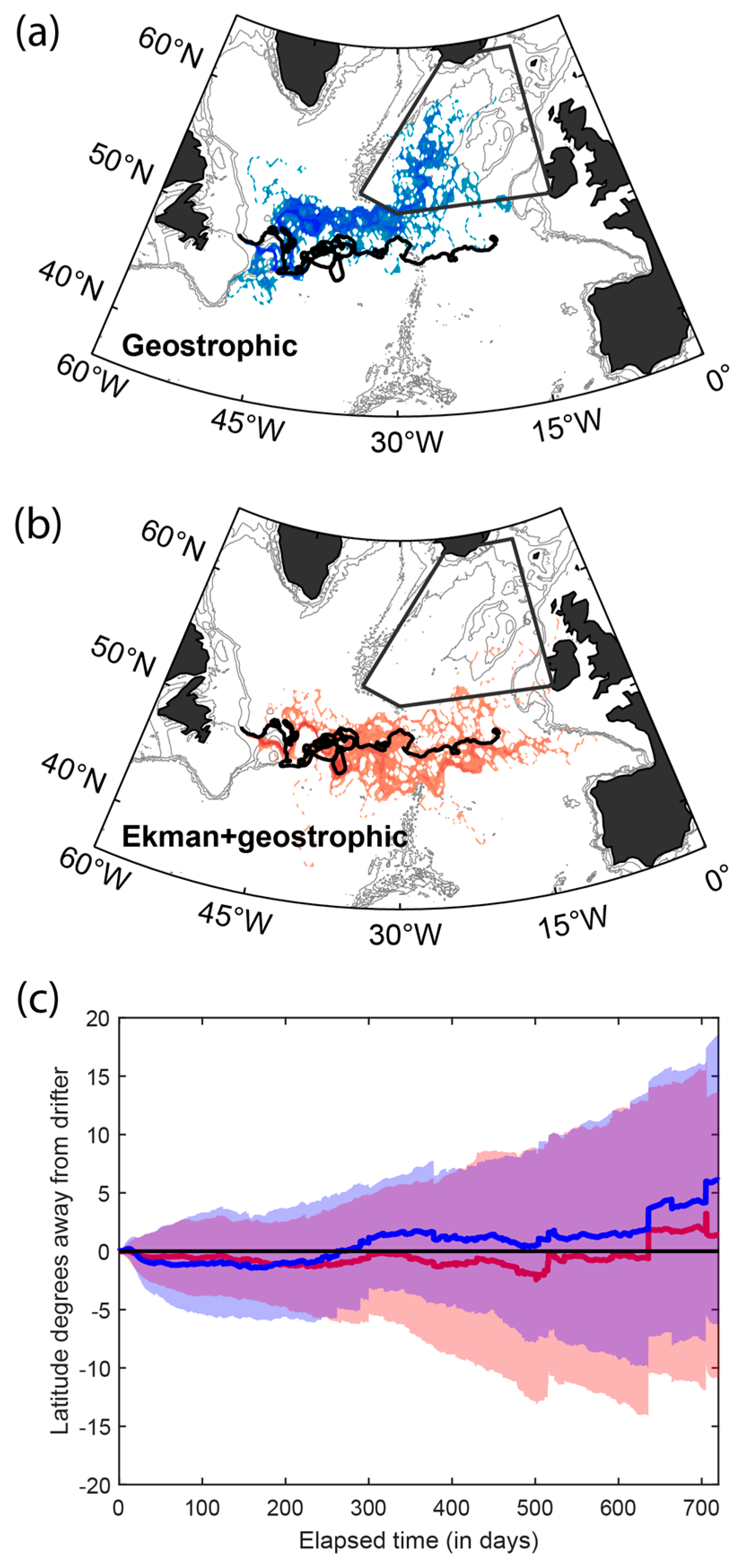
2.4. Ability of Altimetry-Derived Velocity Fields to Predict Surface Drifter Pathways

As a first step in the analysis, we investigated the relative ability of altimetry-based velocity fields to reproduce the general behaviors of surface drifters from the Global Drifter Program. Because we utilized the Ekman+geostrophic velocity field at a depth of 15 m, we selected only drifters drogued at 15 m whose paths intersected our particle initialization line (shown in Figure 2); 163 surface drifters met our criteria and were used for this analysis. For the purposes of this analysis, the “start” location and time of each surface drifter were considered as the moment they crossed our particle initialization line. For each surface drifter, 25 particles were initialized at the exact start time of the surface drifter in a 4 km radius grouping around the surface drifter start location: 1 particle was released at the exact starting location of the drifter, and 24 particles were released in concentric rings of 8 at 1, 2, and 4 km from the drifter’s starting location to test the sensitivity of the calculated trajectories to the initial position. Particle trajectories were calculated for the same duration as the lifespan of the surface drifter. These steps were taken for each of the 163 surface drifters in the geostrophic velocity field and the Ekman+geostrophic velocity field.
To visually demonstrate the relationship between the calculated particle clouds and the observed surface drifter, we show one drifter example with trajectories resulting from both the geostrophic and Ekman+geostrophic velocity fields in Figure 3. In this example, which is exemplary of many other drifter–simulation comparisons considered, the trajectories integrated using the Ekman+geostrophic velocity field replicated the general behavior of the surface drifter well (Figure 3b). This correspondence is notable considering the 1/4° altimetry fields range from 15–30 km spatial resolution, and thus only resolve larger mesoscale processes. Conversely, the trajectories integrated over the geostrophic velocity field tended to skew several latitude degrees north of the surface drifters on average (Figure 3a). The overall trend (Figure 3c) is similar to this single example; the geostrophic trajectories are generally about 4° north of the surface drifters after ~2 years of integration, whereas the Ekman+geostrophic trajectories are generally at the same latitude after a 2-year integration. This can be explained by the fact that the surface drifters are drogued in the Ekman layer, and thus the velocity field that includes the Ekman component is a better model for the surface drifters.

2.5. Geostrophic Versus Ekman+Geostrophic Velocity Fields

Given the large spread between the particle clouds with and without Ekman+geostrophic velocities shown in Figure 3, we aim to determine which velocity field is more indicative of the freshwater pathways we seek to follow in this study. In Figure 4, we map the particle distributions for all the trajectories calculated using the geostrophic (Figure 4a) and Ekman+geostrophic (Figure 4b) velocity fields; all 27,622 particle trajectories are shown with a lifespan of two years after initialization. With all simulation parameters—integration timestep, initial particle locations, and integration length—remaining identical between the two simulations, any differences are isolated to the velocity fields. The difference between panels (Figure 4a) and (Figure 4b) can be attributed to the dominant wind pattern over the mid-latitude North Atlantic. Prevailing westerly winds deflect the surface layer waters southward, causing them to recirculate in the subtropical gyre [30]. Without the Ekman component in the velocity field, particles are more likely to enter the Iceland Basin, a result that aligns with a study of subtropical-to-subpolar exchange in altimetry-derived surface currents [29]. Further, because Holliday et al. (2020) [4] observe the fresh anomaly up to 1000 m below the surface, the geostrophic velocities more closely track the depths that are of interest in this study. Satellite SSH has been shown to be representative of the structure thermocline layer across the subpolar North Atlantic in a direct comparison with hydrographic data referenced to 1000 m [29]. Häkkinen and Rhines (2004) [31] state that altimetry-derived surface currents are indicative of open-ocean currents (direction and speed) from the surface to the thermocline. Building upon this, Desbruyeres et al. (2021) [29], in a model tracer study, concluded that the non-inclusion of the Ekman component of surface velocities “enables the tracers to be strictly advected within a velocity field that primarily reflects the surface-intensified first baroclinic mode and the motions of the main thermocline”, and that altimeter-derived geostrophic sea surface velocity is a “fair proxy of the large-scale upper circulation and its changing intensity and horizontal structure”. For these reasons, the remaining analysis in this paper will focus solely on the trajectories calculated using the geostrophic-only velocity field.

3. Results

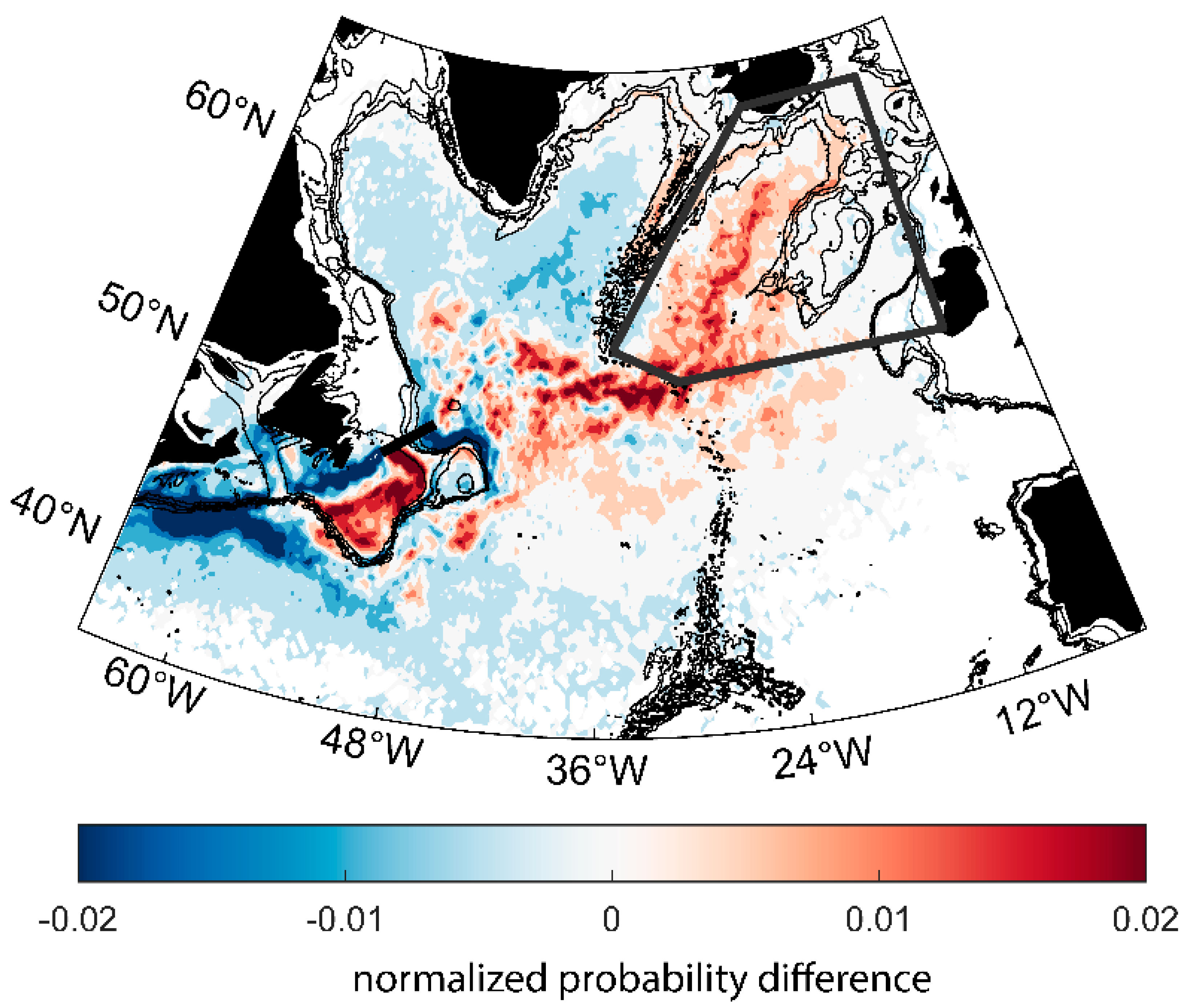
3.1. More Labrador Current-Origin Water Found in Iceland Basin in 2015 and 2016

Trajectories connecting the Labrador Current with the IB/RT (see Figure 1 or Figure 3) provide information on the strength of this connection as a function of time, as well as the speed at which the waters transit between the two locations. Of the 27,622 trajectories initialized in the Labrador Current in the geostrophic velocity fields between 1 January 1993 and 31 December 2019, 11,568 (42%) made it to the IB/RT within two years. The remainder of the particles either (a) passed southwestward into the NWACSS region, (b) crossed the North Atlantic but remained in the subtropical gyre in the West European Basin, or (c) followed the Reykjanes Ridge northward into the Irminger Basin (Table 1).
The majority of particles entering the IB/RT took about 7–11 months to cross the basin, with the fastest particles entering the IB/RT after only 90 days (3.0 months). The distribution of particle ages (Figure 5a) follows a log-normal distribution, with a peak value at 295 days (9.7 months) and a mean of 353 days (11.6 months). The number of particles entering the IB/RT drops considerably after 18 months, but particles continued to arrive to the region after two years.
The time dependence of this age distribution (Figure 5b) demonstrates that the mean and max of these age distributions shortened for particles released between 2010 and 2018, from 12.8 months (distribution mean) and 11.3 months (distribution max) in 2010 to 10.2 months (distribution mean) and 8.1 months (distribution max) in 2018. This 2–3 months (26–28%) shortening of the transit time between the Labrador Current and the IB/RT can also be visualized by an increase in the total number of particles arriving to the IB/RT in those years (Figure 6). From 1995–2007, there were about 370 particles arriving to the IB/RT each year. In 2009, the Labrador Current-origin particles in the IB/RT region increased to over 500, then decreased in 2010, and remained high through 2017. Marked maxima in 2015 and 2016 corresponded to almost a doubling of the number of particles compared to the early 2000s. This time variability corresponds closely with the time derivative of the age distribution time series; an along-stream convergence of particles occurs when a group of particles catches up to the particles released at a prior time. Thus, the consistent shortening of the age distribution from 2010 to 2018 caused a continuously high number of particles arriving to the IB/RT, consistent with a freshening during this time period (Figure 6, the annual average salinity derived from Ellet Line hydrographic data in the density range σ0 = 27.20 to 27.50 kg/m3 (from ~30 m–600 m) [32]). The Holliday et al. (2020) [4] hypothesis that the Iceland Basin freshening event occurred due to more input from the Labrador Current is consistent with these results, and we are able to further show that this increase was due to younger particles arriving to the IB/RT, potentially carrying with them even fresher waters than the longer-duration particles.

3.2. Labrador Current Waters Diverted East at the Tail of the Grand Banks between 2012–2016

A shorter transit time from the Labrador Current could be caused by either a shift in the pathways of the particles or a speeding up of the existing pathways. To determine if the pathways to the IB/RT shifted during this time period, we separated the trajectories into pathways, using the probability distribution function of all calculated trajectories in the geostrophic velocity field (Figure 4a) to guide our choices. There are two apparent pathways that direct Labrador Current-origin waters toward the eastern SPNA. The most popular pathway departs the shelfbreak north of the Flemish Cap and continues northeastward toward the Iceland Basin—a “direct” pathway into the NAC. Trajectories classified in this pathway must have first crossed a meridional line segment spanning from the northern edge of the 200 m isobath on the Flemish Cap to 54°N, shown in Figure 7b with example trajectories. The statistics of these direct pathway trajectories are provided in Table 1.
The second pathway, coined by Fox et al. (2022) [19] as the “looped” pathway, is significantly less direct, taking particles through the Flemish Pass on the shelfbreak, and retroflecting inshore of the Gulf Stream to eventually join the NAC (Figure 7c). Trajectories are classified as looped if they crossed eastward through a meridional line at 45°W between 42°N and 47.5°N. Within this looped classification, there were multiple pathways that the particles followed, so we further divided this looped pathway into a group that left the shelfbreak east of the TGB, and a group that left the shelf west of the TGB. Surprisingly, the fastest pathway from the Labrador Current launch site and the IB/RT was this looped “East TGB” pathway; this was a faster route to the IB/RT than the so-called direct pathway, while the looped “West TGB” pathway was the slowest pathway.
Though the majority of calculated trajectories moved east—either before reaching the Tail of the Grand Banks, or by retroflecting back east after tracing it west—about a quarter of the trajectories instead continued westward from the TGB, ultimately residing in the NWACSS region, including the Gulf of St. Lawrence, the Scotian Shelf, and the Gulf of Maine (Figure 7d). Trajectories were classified as following this west pathway if, after two years of travel, they resided west of the line segment connecting the SW corner of Labrador to the tip of the TGB to 38°N. Finally, a few particles did not fall into any of the three groups defined above, and either recirculated in the Labrador Sea, or were advected from the launch site inshore prior to reaching the Grand Banks.
Observing an elevated number of trajectories entering the IB/RT between 2012 and 2016 prompted further investigation into the changes in these three pathways—direct, looped, and western—as a function of time. The number of trajectories classified in each pathway was calculated annually from 1993 to 2020 (Figure 7a). The direct pathway was consistently between 400 and 500 particles per year throughout the 27-year time series, with peaks in 1999, 2007, and 2015. The largest peak occurred in 2015, corresponding closely to the maximum in total IB/RT particles (Figure 6). To explain the peak in IB/RT particles arriving in 2009, one must consider the looped and western pathways. There is a notable anticorrelation between these two pathways, and a shift in 2009 when more particles followed the looped pathway (a 55% increase from 220 particles in 2006–2008 to 340 particles in 2009) rather than the western pathway (a correspondingly large decrease). This shift from the western pathway to the looped pathway in 2009 was largely due to an increase in particles following the looped “East TGB” pathway, though it was later followed by an increase in the looped “West TGB” pathway in 2011. This partitioning between the looped and west pathways remained relatively flat through 2019.
To map the spatial patterns apparent in these pathways, we show the probability distribution function of all particle trajectories initiated between 2012 and 2016 subtracted from the probability distribution function of all particle trajectories initiated between 2003 and 2007 (Figure 8). These periods were chosen to represent a baseline state and the freshening period. Maps of mean surface velocity for time periods 2003–2007 and 2012–2016 (not shown) do not show as clearly the change in circulation pattern that is detected with the Lagrangian approach. The spatial distribution of trajectories between 2012 and 2016 demonstrates comparable patterns to that shown in Holliday et al. (2020) [4]: the Iceland Basin and NAC jets experience an anomalously high probability of Labrador-origin trajectories in 2012–2016, and the NWACSS experiences a lower probability of trajectories in 2012–2016 than in prior reference periods. Of particular interest, however, are the relative strengthening and weakening of the three major pathways of Labrador Current-origin particles around the Grand Banks. The western pathway that meanders across the Grand Banks was significantly less traveled in 2012–2016. The looped pathway that departs the shelfbreak and retroflects inshore of the Gulf Stream was amplified during 2012–2016. The direct pathway that departs the shelfbreak north of the Flemish Cap was less traveled in 2012–2016. This decrease in the direct pathway is at first glance contrary to the apparent consistent arrival of particles from that pathway to the IB/RT. However, there is a coincident increase in particles north of the direct path along the slope, and an increase in particle incidence at the northern part of the Flemish Cap—both locations also satisfy the “direct gate” criterion.
In addition to this shift in pathways to more looped “East TGB” pathways, the pathways also sped up starting in 2009 (Figure 9). This is most apparent in the “Direct” pathway in which the mean age decreased from 12.25 months in 2010 to 9.7 months in 2015, and the “Looped East TGB” pathway in which the mean age decreased from 11.6 months in 2010 to 8.5 months in 2016. So not only were more particles taking these routes, but the routes also sped up.

4. Discussion

4.1. Diversion Mechanisms near the Tail of the Grand Banks

Our findings demonstrate a rapid change in the pathways of Labrador Current-origin water near the Tail of the Grand Banks beginning in 2009, marked by an increase in trajectories retroflecting eastward at the TGB, and a concomitant decrease in trajectories moving west onto the NWACSS (Figure 6, Figure 7 and Figure 8). These spatial shifts in the pathways were accompanied by an increase in the speed of the pathways that led to the IB/RT, which resulted in an along-stream convergence and further enhanced the Labrador Current’s influence in the eastern SPNA (Figure 9). These results are consistent with the diversion hypothesis put forward by Holliday et al. (2020) [4]. The rapid change in 2009 toward a regime where Labrador Current-origin water at the Tail of the Grand Banks is diverted eastward instead of westward might suggest a mechanism for the overwhelming arrival of Labrador Current-origin particles in the Iceland Basin in 2015 and 2016; however, the period of “recovery” to normal salinity following the 2012–2016 freshening event is not as straightforward. Upper layer salinity in the Iceland Basin reached a distinct minimum in 2017, followed by a sharp trend toward a more typical, though still slightly fresh, salinity from 2018–2021. Fewer Labrador Current-origin waters arrived during these later years, mostly driven by fewer “Direct” pathway particles, but also fewer “Looped East TGB” particles by 2020. Another factor in the subsequent rebound of the salinity in the Iceland Basin is a slowing of the pathways: the “Looped East TGB” pathway slowed from 8.5 months to 10.0 months from 2016 to 2017, and the “Direct” pathway slowed from 9.9 months in 2018 to 10.9 months in 2019. A slowing of the pathways has two effects: (1) fewer particles arrive to the region while the slowing is occurring, and (2) the waters in the pathway likely become saltier as they mix with the NAC waters [33]. These changes were accompanied by a large-scale shift in the NAC that brought more subtropical waters northward into the eastern SPNA [29].
The rapidity of the freshening in 2009, posited by Holliday et al. (2020) [4], can be described by changes in wind stress curl associated with a strong winter NAO index, the conditions of which descended rapidly on the SPNA in the winter of 2010 and shifted the subpolar front of the Newfoundland Basin south by 2011, when the fresh anomaly is first observed there. The effect described by Holliday et al. (2020) [4] is a strong Ekman transport of Labrador Current-origin waters off the Newfoundland shelf and into the NAC, which aligns closely with observed propagation of the fresh anomaly to the eastern SPNA in the Extended Ellett and OVIDE line hydrographic observations. Following the increased Ekman transport off the shelf, Holliday et al. (2020) [4] describe a rapid shift to a positive NAO index in 2014, resulting in an expansion of the subpolar gyre: the subpolar front shifted to the southern NAC branch (typically, it sits at the northern branch), which extended further eastward and transported the bulk of the wind-driven freshwater anomaly away from the Newfoundland Shelf and into the eastern SPNA.
The expansion of the subpolar gyre, which Holliday et al. (2020) [4] defines as the spread of relatively cold, fresh water, was observed in the eastern basins as the southern branch of the NAC extended eastward and increased velocity and transport of the fresh anomaly. Closer to the TGB, however, the subpolar boundary between the Gulf Stream and the Labrador Current may also experience changes in location and strength. Gonçalves-Neto et al. (2021) [17] reported an anomalously high sea level at the TGB since the summer of 2008, suggesting an inshore migration of the Gulf Stream. Labrador Current-origin waters that might otherwise continue west toward the NWACSS may be blocked by the inshore migration of the Gulf Stream, resulting in higher temperatures (and higher salinity) on the NWACSS. Because our results illustrate a rapid decrease in trajectories reaching the NWACSS and a concurrent increase in trajectories retroflecting east toward the NAC in 2009, the inshore migration of the Gulf Stream provides another means of eastward transport beyond that of Ekman transport off the shelves. It is worth noting that Gonçalves-Neto et al. (2021) [17] utilize the same altimetry-based sea surface height dataset from which the velocity field we use is derived, which may account for some degree of agreement in our results. Another altimetry-based metric of the subpolar gyre size also captures a shift around 2009 near the Grand Banks that is consistent with the pathway shift described herein: the southward extent of closed SSH contours around the subpolar gyre contracted northward in 2009 from extending around the TGB to splitting off the shelfbreak to the east of the TGB [34]. Thus, it appears that this offshore shift of the Labrador Current in 2009 is apparent in a variety of altimetry-based metrics.

4.2. Expanding insights from Surface to Depth

Our decision to utilize altimetry-derived velocity products offers both advantages and drawbacks that affect the application of our results. Notably, the 1/4° spatial resolution of the altimetry fields limits our ability to understand processes smaller than the smaller half of the mesoscale spectrum (<25 km). In addition, though altimetry on the inner shelf may be questionable due to the smaller spatial scales, sharper bathymetry, and importance of the geoid models, we took measures to avoid utilizing on-shelf velocity data. Integrating particles through the geostrophic velocity field allows for calculation of particle locations based on observations instead of model data. Recently published studies have simulated the movement of particles in high-resolution models [18,19] and ocean re-analyses [21] to gain insights into the source of the 2012–2016 SPNA freshening. Because the 2012–2016 freshwater anomaly was observed from the surface ocean to a depth of 1000 m, the ability to initialize and track particles at depth using three-dimensional velocity fields offers unique insights that altimetry-derived velocity fields alone cannot provide. Yet, a tracer experiment comparing the altimetry-derived geostrophic velocity field and ECCOv4r4 led Desbruyères et al. (2021) [29] to conclude that altimetry-derived geostrophic surface velocity is representative of large-scale pathways in the upper ocean from the surface down to the pycnocline. Our comparisons with observed surface drifters provide some insight about the capability of particle integration through altimetry-derived velocity fields, but the lack of isobaric or isopycnal observational tools at depth within the region of interest and availability of altimetry made it difficult to draw conclusions about the ability to reproduce trajectories below the surface.

5. Conclusions

Particle trajectories originating in the Labrador Current and integrated forward in time using altimetry-derived surface velocity fields entered the Iceland Basin during the 2012–2016 freshening event at nearly twice the frequency observed prior to 2009 (see Figure 6), suggesting an increased presence of Labrador Current-origin water in the Iceland Basin and Rockall Trough during the observed freshening. Further, we observed a distinct regime change in 2009 that saw a decrease in trajectories that went west at the Tail of the Grand Banks and a concurrent increase in trajectories that retroflected east into the NAC, suggesting a diversion of Labrador Current-origin waters eastward (see Figure 7 and Figure 8). These spatial shifts were accompanied by faster transit times along the pathways which led to along-stream convergence and more particles arriving to the eastern subpolar gyre (see Figure 9). Regions of anomalous freshening (Iceland Basin, Rockall Trough) align with the increased presence of calculated trajectories in 2012–2016, and regions of anomalous salinification along the Scotian Shelf and Gulf of Maine [4,35] align with the decreased presence of calculated trajectories during the same time. These observation-based results support the Holliday et al. (2020) [4] hypothesis that diversion of relatively fresh Labrador Current waters eastward from the western boundary of the subpolar North Atlantic contributed to the unprecedented freshening in the Iceland Basin.

Author Contributions

H.H.F. and N.P.F. contributed equally to the manuscript. Conceptualization, A.S.B.; methodology, A.S.B., H.H.F. and N.P.F.; software, A.A., N.P.F. and H.H.F.; validation, A.A., N.P.F. and H.H.F.; formal analysis, N.P.F., A.A. and H.H.F.; investigation, A.A., N.P.F. and H.H.F.; resources, A.S.B. and N.P.F.; data curation, A.A., N.P.F. and H.H.F.; writing—original draft preparation, A.A., N.P.F. and H.H.F.; writing—review and editing, H.H.F., N.P.F. and A.S.B.; visualization, A.A., H.H.F. and N.P.F.; supervision, A.S.B., H.H.F. and N.P.F.; project administration, A.S.B., H.H.F. and N.P.F.; funding acquisition, A.S.B. and N.P.F. All authors have read and agreed to the published version of the manuscript.

Funding

This research was funded by the National Science Foundation, grant OCE 2123128 for N.F. and grant OCE 1756361 for A.S.B., H.H.F. and A.A.

Data Availability Statement

Publicly available datasets were analyzed in this study. The Copernicus Marine Service surface geostrophic velocity field with ¼-degree resolution data can be found here: https://doi.org/10.48670/moi-00148 (accessed on 22 June 2022). The Copernicus Marine Service geostrophic velocity field with Ekman component can be found here: https://doi.org/10.48670/mds-00327 (accessed on 12 July 2022). Restrictions apply to the availability of the Bonavista Line data. Data were obtained from Frédéric Cyr and are available from the authors with the permission of Cyr.

Acknowledgments

The authors thank Cyr for providing hydrographic data from the Bonavista Line.

Conflicts of Interest

The authors declare no conflict of interest.

References

  1. Gelderloos, R.; Straneo, F.; Katsmann, C.A. Mechanisms behind the temporary shutdown of deep convection in the Labrador Sea: Lessons from the Great Salinity Anomaly Years 1968–1971. J. Clim. 2012, 25, 6743–6755. [Google Scholar] [CrossRef]
  2. Böning, C.; Behrens, E.; Biastoch, A.; Getzlaff, K.; Bamber, J.L. Emerging impact of Greenland meltwater on deepwater formation in the North Atlantic Ocean. Nat. Geosci. 2016, 9, 523–552. [Google Scholar] [CrossRef]
  3. Yang, Q.; Dixon, T.H.; Myers, P.G.; Bonin, J.; Chambers, D.; van den Broeke, M.R.; Ribergaard, M.H.; Mortensen, J. Recent increases in Arctic freshwater flux affects Labrador Sea convection and Atlantic overturning circulation. Nat. Commun. 2016, 7, 10525. [Google Scholar] [CrossRef] [PubMed]
  4. Holliday, N.P.; Bersch, M.; Berx, B.; Chafik, L.; Cunningham, S.; Florindo-López, C.; Hátún, H.; Johns, W.E.; Josey, S.A.; Larsen, K.M.H.; et al. Ocean Circulation causes the largest freshening event for 120 years in eastern subpolar North Atlantic. Nat. Commun. 2020, 11, 585. [Google Scholar] [CrossRef] [PubMed]
  5. Biló, T.C.; Straneo, F.; Holte, J.; Le Bras, I.A.-A. Arrival of new great salinity anomaly weakens convection in the Irminger Sea. Geophys. Res. Lett. 2022, 49, e2022GL098857. [Google Scholar] [CrossRef]
  6. Le Bras, I.A.-A.; Straneo, F.; Holte, J.; De Jong, M.F.; Holliday, N.P. Rapid export of waters formed by convection near the Irminger Sea’s western boundary. Geophys. Res. Lett. 2020, 47, 3. [Google Scholar] [CrossRef]
  7. Dickson, R.R.; Meincke, J.; Malmberg, S.-A.; Lee, A.J. The “Great Salinity Anomaly” in the Northern North Atlantic 1968–82. Prog. Oceanogr. 1988, 20, 103–151. [Google Scholar] [CrossRef]
  8. Belkin, I.M.; Levitus, S.; Antonov, J.; Malmberg, S.-V. “Great Salinity Anomalies” in the North Atlantic. Prog. Oceanogr. 1998, 41, 1–68. [Google Scholar] [CrossRef]
  9. Belkin, I.M. Propagation of the “Great Salinity Anomaly” of the 1990s around the northern North Atlantic. Geophys. Res. Lett. 2004, 31, L08306. [Google Scholar] [CrossRef]
  10. Lazier, J.R. Oceanographic conditions at ocean weather ship Bravo, 1964–1974. Atmos.-Ocean 1980, 18, 227–238. [Google Scholar] [CrossRef]
  11. Haak, H.; Jungclaus, J.; Mikolajewicz, U.; Latif, M. Formation and propagation of great salinity anomalies. Geophys. Res. Lett. 2003, 30, 9. [Google Scholar] [CrossRef]
  12. Holliday, N.P.; Hughes, S.L.; Bacon, S.; Beszczynska-Möller, A.; Hansen, B.; Lavín, A.; Loeng, H.; Mork, K.A.; Østerhus, S.; Sherwin, T.; et al. Reversal of the 1960s to 1990s freshening trend in the northeast North Atlantic and Nordic Seas. Geophys. Res. Lett. 2008, 35, 3. [Google Scholar] [CrossRef]
  13. Fratantoni, P.S.; Pickart, R.S. The western North Atlantic shelfbreak current system in summer. J. Phys. Oceanogr. 2007, 37, 2509–2533. [Google Scholar] [CrossRef]
  14. Han, G.; Ma, Z.; Chen, N. Ocean climate variability off Newfoundland and Labrador over 1979–2010: A modelling approach. Ocean Model. 2019, 144, 101505. [Google Scholar] [CrossRef]
  15. Fratantoni, P.S.; McCartney, M.S. Freshwater export from the Labrador Current to the North Atlantic Current at the Tail of the Grand Banks of Newfoundland. Deep-Sea Res. I. 2009, 57, 258–283. [Google Scholar] [CrossRef]
  16. Wang, Q.; Ilicak, M.; Gerdes, R.; Drange, H.; Aksenov, Y.; Bailey, D.A.; Bentsen, M.; Biastoch, A.; Bozec, A.; Böning, C.; et al. An assessment of the Arctic Ocean in a suite of interannual CORE-II simulations. Part II: Liquid freshwater. Ocean Model. 2016, 99, 86–109. [Google Scholar] [CrossRef]
  17. Gonçalves Neto, A.; Langan, J.A.; Palter, J.B. Changes in the Gulf Stream preceded rapid warming of the Northwest Atlantic Shelf. Commun. Earth Environ. 2021, 2, 74. [Google Scholar] [CrossRef]
  18. Gonçalves Neto, A.; Palter, J.B.; Xu, X.; Fratantoni, P. Temporal variability of the Labrador Current pathways around the Tail of the Grand Banks at intermediate depths in a high-resolution ocean circulation model. J. Geophys. Res. Ocean. 2023, 128, 3. [Google Scholar] [CrossRef]
  19. Fox, A.D.; Handmann, P.; Schmidt, C.; Fraser, N.; Rühs, S.; Sanchez-Franks, A.; Martin, T.; Oltmanns, M.; Johnson, C.; Rath, W.; et al. Exceptional freshening and coolingin the eastern subpolar North Atlantic caused by reduced Labrador Sea surface heat loss. Ocean Sci. 2022, 18, 1507–1533. [Google Scholar] [CrossRef]
  20. Biastoch, A.; Schwarzkopf, F.U.; Getzlaff, K.; Rühs, S.; Martin, T.; Scheinert, M.; Schulzki, T.; Handmann, P.; Hummels, R.; Böning, C. Regional imprints of changes in the Atlantic Meridional Overturning Circulation in the eddy-rich ocean model VIKING20x. Ocean Sci. 2021, 17, 1177–1211. [Google Scholar] [CrossRef]
  21. Jutras, M.; Dufour, C.; Mucci, A.; Talbot, L.C. Large-scale control of the retroflection of the Labrador Current. Nat. Commun. 2023, 14, 2623. [Google Scholar] [CrossRef] [PubMed]
  22. Reagan, J.R.; US DOC/NOAA/NESDIS/NCEI > Oceanographic and Geophysical Science and Services Division. World Ocean Atlas 2023—Objectively Analyzed In Situ Temperature and Salinity Climatologies for the 1991–2020 Climate Normal Period (NCEI Accession 0270533). Subset 1991–2000 Climatology. NOAA National Centers for Environmental Information. 2020. Available online: https://www.ncei.noaa.gov/archive/accession/0270533 (accessed on 5 July 2023).
  23. Rio, M.-H.; Mulet, S.; Picot, N. Beyond GOCE for the ocean circulation estimate: Synergistic use of altimetry, gravimetr, and in situ data provides new insight into geostrophic and Ekman currents. Geophys. Res. Lett. 2014, 41, 24. [Google Scholar] [CrossRef]
  24. Cyr, F.; Snook, S.; Bishop, C.; Galbraith, P.S.; Chen, N.; Han, G. Physical Oceanographic Conditions on the Newfoundland and Labrador Shelf during 2021. DFO Can. Sci. Advis. Secr. Res. Doc. 2022. Available online: https://waves-vagues.dfo-mpo.gc.ca/library-bibliotheque/41063491.pdf (accessed on 6 December 2023).
  25. Florindo-Llopez, C.; Bacon, S.; Aksenov, Y.; Chafik, L.; Colbourne, E.; Holliday, N.P. Arctic Ocean and Hudson Bay freshwater exports: New estimates from seven decades of hydrographic surveys on the Labrador Shelf. J. Clim. 2020, 33, 8849–8868. [Google Scholar] [CrossRef]
  26. Delandmeter, P.; Van Sebille, E. The Parcels v2.0 Lagrangian framework: New field interpolation schemes. Geosci. Model Dev. 2019, 12, 3571–3584. [Google Scholar] [CrossRef]
  27. Wagner, P.; Rühs, S.; Schwarzkopf, F.U.; Koszalka, I.M.; Biastoch, A. Can Lagrangian tracking simulate tracer spreading in a high-resolution ocean general circulation model? J. Phys. Oceanogr. 2019, 49, 1141–1157. [Google Scholar] [CrossRef]
  28. Schmidt, C.; Schwarzkopf, F.U.; Rühs, S.; Biastoch, A. Characteristics and robustness of Agulhas leakage estimates: An inter-comparison study of Lagrangian methods. Ocean Sci. 2021, 17, 1067–1080. [Google Scholar] [CrossRef]
  29. Desbruyères, D.; Chafik, L.; Maze, G. A shift in the ocean circulation has warmed the subpolar North Atlantic Ocean since 2016. Commun. Earth Environ. 2021, 2, 48. [Google Scholar] [CrossRef]
  30. Brambilla, E.; Talley, L.D. Surface drifter exchange between the North Atlantic subtropical and subpolar gyres. J. Geophys. Res. Ocean. 2006, 111, C7. [Google Scholar] [CrossRef]
  31. Hakkinen, S.; Rhines, P.B. Decline of subpolar North Atlantic circulation during the 1990s. Science 2004, 304, 555–559. [Google Scholar] [CrossRef]
  32. Holliday, N.P.; Cunningham, S.; Johnson, C.; Gary, S.F.; Griffiths, C.; Read, J.F.; Sherwin, T. Multidecadal variability of potential temperature, salinity and transports in the eastern subpolar North Atlantic. J. Geophys. Res. Ocean. 2015, 120, 5945–5967. [Google Scholar] [CrossRef]
  33. Berglund, S.; Döös, K.; Groeskamp, S.; McDougall, T. North Atlantic Ocean Circulation and Related Exchange of Heat and Salt Between Water Masses. Geophys. Res. Lett. 2023, 50, 13. [Google Scholar] [CrossRef]
  34. Foukal, N.P.; Lozier, M.S. Assessing variability in the size and strength of the North Atlantic subpolar gyre. J. Geophys. Res. Ocean. 2017, 122, 8. [Google Scholar] [CrossRef]
  35. Gawarkiewicz, G.; Fratantoni, P.; Bahr, F.; Ellertson, A. Increasing frequency of salinity maximum intrusions in the Middle Atlantic Bight. J. Geophys. Res. Ocean. 2022, 127, 7. [Google Scholar] [CrossRef]
Figure 2. (a) Practical salinity from the June 2000 Bonavista Line, a repeat hydrographic section regularly sampled by the Atlantic Zone Monitoring Program (AZMP) [24]. The location of the Bonavista Line is shown on subplot (c). Approximate deployment location resolution is plotted as black triangles along the top of the plot. (b) Same, but for potential temperature referenced to 0 dbar. (c) Mean geostrophic velocity field spanning 1993–2021 is depicted at the native ¼° resolution of the gridded product derived from SSH. Particle deployment locations are indicated as white circles, Bonavista station locations (upstream, northwest of the particle deployment locations) are plotted as gray squares. The 200 m, 500 m, 1000 m, and 2000 m isobaths are plotted, and this convention is used in all subsequent geographic plots.
Remotesensing 15 05711 g002
Figure 3. Comparison of surface drifters and particles calculated from the altimetry-derived surface currents. (a,b) depict examples of Drifter #1764 and the cloud of 25 released particles at 1 km, 2 km, and 4 km surrounding the point of crossing the deployment line using both the geostrophic and Ekman+geostrophic velocity fields, respectively. (c) The average and standard deviation of latitude distance between all drifters and the associated cloud of 25 simulations for the geostrophic velocity (blue) and Ekman+geostrophic velocity field (red). Because the surface drifters are drogued within the Ekman layer, the Ekman velocity fields more closely mimic the surface drifter trajectories.
Remotesensing 15 05711 g003
Figure 4. Normalized probability distributions of all trajectories calculated using the (a) geostrophic velocity field and the (b) combined Ekman+geostrophic velocity fields. The region shown was divided into grid areas of ¼° and the fraction of particles visiting each grid square is depicted, discounting repeat visits by the same particle. The polygon demarcating the IB/RT is shown in black.
Remotesensing 15 05711 g004
Figure 5. The age distribution of particles that enter the IB/RT. (a) The number of particles arriving to the IB/RT in 5-day bins of particle age calculated over all years. The log-normal fit and its mean and max values are shown. (b) Time variability of the mean and maxima of each year’s age distribution plot. Particle dates are shown by their year of initialization in the Labrador Current.
Remotesensing 15 05711 g005
Figure 6. Time series showing the annual (black) and seasonal (gray) sum of the number of calculated trajectories that reached the IB/RT polygon at time of entry into the IB/RT polygon (black line). The seasons are defined as January–February–March, April–May–June, July–August–September, and October–November–December. The blue line indicates the annual surface salinity in the Iceland Basin for the density range σ0 = 27.20 to 27.50 kg/m3 (from ~30 m–600 m) derived from the Extended Ellett Line stations located in the Iceland Basin [32]. The 2003–2007 and 2012–2016 time periods are highlighted light red and light blue, respectively.
Remotesensing 15 05711 g006
Figure 7. (a) Annual time series of the number of particles (at time of release) following the three major pathways from the Grand Banks, with the 2003–2007 reference period shaded in red (see text) and the 2012–2016 Iceland Basin freshening event shaded in blue. Yellow: direct pathway, blue: west pathway, red: looped pathway. The looped pathway is further decomposed into particles that looped east (thin red line) or west (thin dashed red line) of the TGB. Example trajectories chosen randomly over the study period are displayed to illustrate each of the three major pathways of Labrador Current-origin particles. Pathways include (b) the direct pathway, (c) the looped pathway, and (d) the west pathway. The IB/RT box and the gates used to categorize pathways (see text) are drawn in panels (bd) for reference.
Remotesensing 15 05711 g007
Figure 8. Normalized difference in the probability distribution of trajectories between 2012–2016 (freshening event) and 2003–2007 (reference period). The reference period was chosen to be representative of the number of trajectory arrivals in the IB/RT prior to 2009, when the offshore shift occurred. Shades in red indicate a positive difference (e.g., more 2012–2016 trajectory probability than 2003–2007); shades in blue indicate a negative difference (e.g., lower 2012–2016 trajectory probability than 2003–2007). The two time periods used in this comparison are highlighted in Figure 6 and Figure 7.
Remotesensing 15 05711 g008
Figure 9. Time series of age distributions for each pathway: (a) Direct, (b) Looped, (c) Looped “East TGB”, and (d) Looped “West TGB”.
Remotesensing 15 05711 g009
Table 1. Statistics of trajectory pathways.
PathwayPercent of Total TrajectoriesPercent of Total Trajectories That Reached IB/RTPeak (Mean) Travel Time to IB/RT
All100%42%295 d (353 d)
Direct43%25%275 d (331 d)
Looped30%17%320 d (385 d)
West of TGB7%5%365 d (429 d)
East of TGB22%11%255 d (305 d)
West26%--
None2%--
Disclaimer/Publisher’s Note: The statements, opinions and data contained in all publications are solely those of the individual author(s) and contributor(s) and not of MDPI and/or the editor(s). MDPI and/or the editor(s) disclaim responsibility for any injury to people or property resulting from any ideas, methods, instructions or products referred to in the content.

