Article

Reconstructing the Three-Dimensional Structure of Loop Current Rings from Satellite Altimetry and In Situ Data Using the Gravest Empirical Modes Method

1
Woods Hole Oceanographic Institution, Woods Hole, MA 02543, USA
2
Centro de Investigacion Cientifica y de Educacion Superior de Ensenada, Ensenada 22860, Mexico
*
Author to whom correspondence should be addressed.
Remote Sens. 2022, 14(17), 4174; https://doi.org/10.3390/rs14174174
Submission received: 1 July 2022 / Revised: 9 August 2022 / Accepted: 16 August 2022 / Published: 25 August 2022
(This article belongs to the Special Issue Remote Sensing Applications in Ocean Observation)

Abstract

:
The three-dimensional structure of Gulf of Mexico’s warm-core rings, detaching from the Loop Current, is investigated using satellite altimetry and a large set of ARGO float profiles. Reconstruction of the Loop Current rings (LCRs) vertical structure from sea surface height observations is made possible by the use of the gravest empirical modes method (GEM). The GEMs are transfer functions that associate a value of temperature and salinity for each variable pair {dynamic height; pressure}, and are computed by estimating an empirical relationship between dynamic height and the vertical thermohaline structure of the ocean. Between 1993 and 2021, 40 LCRs were detected in the altimetry and their three-dimensional thermohaline structure was reconstructed, as well as a number of dynamically relevant variables (geostrophic and cyclogeostrophic velocity, relative vorticity, potential vorticity, available potential energy and kinetic energy density, etc.). The structure of a typical LCR was computed by fitting an analytical stream function to the LCRs dynamic height signature and reconstructing its vertical structure with the GEM. The total heat and salt contents and energy of each LCR were computed and their cumulative effect on the Gulf of Mexico’s heat, salt and energy balance is discussed. We show that LCRs have a dramatic impact on these balances and estimate that residual surface heat fluxes of −13 W m 2 are necessary to compensate their heat input, while the fresh water outflow of the Mississippi river approximately compensates for their salt excess input. An average energy dissipation of O [ 10 10 10 9 ] W kg 1 would be necessary to balance their energy input.

1. Introduction

Although the circulation of the world ocean is dominated by geostrophic turbulence, which is transient by nature, long lived coherent mesoscale eddies can be found in virtually every oceanic basin (e.g., Agulhas rings in the South Atlantic [1,2], Gulf Stream rings in the North Atlantic [3,4], Kuroshio rings in the North Pacific [5,6], Loop Current rings in the Gulf of Mexico [7,8]). Because of their longevity and coherence, these eddies are able to trap and transport tracers (heat, salt, oxygen, plankton, nutrients) far away across basins [2,9,10]. The advent of satellite altimetry in the early 1990s yielded a dramatic increase in the knowledge and understanding of the surface properties of mesoscale eddies [11]. However, energy and tracer transport is by essence a three-dimensional process, as momentum and tracer distribution within mesoscale structures is clearly baroclinic. Understanding and quantifying the role of mesoscale coherent eddies in tracer transports requires a detailed assessment of their vertical structure. Although ship and glider surveys can offer occasional detailed pictures of a limited number of eddies, the observations they provide are too limited in time and space for systematic statistical analysis on a regional or global scale. To address this setback in the availability of a solid statistical description of the three-dimensional properties of mesoscale eddies, a statistical method using jointly in situ observations from ARGO profiling floats and surface observations of sea surface height (SSH) from satellite altimetry were developed [12]. The method consists of automatically detecting mesoscale eddies as closed sea level anomaly (SLA) contours, and searching for ARGO profiles within, and in the vicinity of, the eddy’s boundary. The position of the profile is then referenced to the eddy’s rotation axis and normalized by the eddy’s radius or simply localized by its zonal and meridional distance. Given a sufficient number of profiles, the method allows for the computation of one mean 3-dimensional profile, supposed to be representative of a typical eddy in a given region. The method has since been extensively used in many regions of the ocean ([13,14,15] in the tropical and sub-tropical Pacific, [16]) in the South China sea, [17] in the Arabian sea, [18] in the South Atlantic, [19] in the Lofoten basin, among many). Although the method, known as composite or co-location method, greatly helped to quantify regional statistical properties of mesoscale eddies, they are of limited use, because they only allow for the computation of one average eddy, and not for the reconstruction of the vertical structure of each eddy spotted in the altimetry. Recently, Meunier et al. [20] proposed an alternative method for the estimation of the heat anomaly carried by Loop Current rings (LCR) in the Gulf of Mexico (GoM), based on satellite altimetry and in situ data. Taking advantage of a convenient linear relationship between the local heat content anomaly and SSH, they were able to estimate the total heat content anomaly of each individual eddy. Their method was limited to vertically integrated quantities, and did not provide a full three-dimensional picture of the eddies structure. It could, thus, not provide any information on the energetics of LCRs.
Over two decades ago, Watts et al. [21] and Sun and Watts [22] proposed a method to estimate the full water column’s thermohaline structure from dynamic height observations only. The procedure, known as the Gravest Empirical Modes (GEM), consists in establishing an empirical relationship between dynamic height and temperature and salinity, at a given pressure level, from in situ observations. In the Antarctic circumpolar region, the GEM representation was shown to account for over 97% of the thermohaline variance. Taking advantage of the close relationship between dynamic height and sea surface height, Swart et al. [23] use the GEM methods to reconstruct vertical hydrographic transects in the Antarctic Circumpolar Current from satellite altimetry. More recently, Müller et al. [24] used the GEM method along with satellite altimetry to estimate the heat and fresh water transport by mesoscale eddies in the subpolar north Atlantic. This method is of particular interest because it allows the computation of the thermohaline structure of each individual eddy.
In this study, we follow the procedure of Müller et al. [24], to infer the three-dimensional thermohaline structure of mesoscale eddies, as well as their heat and salt anomalies, and extend it to the computation of other relevant variables, such as geostrophic and cyclogeostrophic velocity, relative vorticity, potential vorticity, as well as kinetic and available potential energy density.
The data used are described in Section 2 and the methods in Section 3. Validation using independent glider observation across an LCR is presented in Section 4. The method is then applied to the 29 years-long AVISO altimetry record in the GoM, where we identified and reconstructed 40 Loop Current rings. The vertical structure of a typical LCR is presented in Section 5 and the statistical properties of LCRs characteristics, with an emphasis on their heat, salt, and energy contents, are presented in Section 6.

2. Data

2.1. In Situ Data

In situ temperature and salinity data were obtained from 6792 ARGO profiles in the Gulf of Mexico. The profiles locations are shown on the map of Figure 1a, showing a wide coverage of the GoM and a homogeneous distribution of the collected data. The color coding corresponds to the local steric height referenced to 2000 dbar computed from the profile data. The presence of the Loop Current (LC) is evident as a tongue of high steric height extending northward from the Yucatan channel and bounded by the West Florida and Louisiana shelves to the East and North, respectively. Sparse high steric height values can also be found in the central and western basin and are the signature of detached LCRs drifting westward. Figure 1b shows a TS diagram of all ARGO profiles. Color coding is the same as in Figure 1a. High steric height water columns are characterized by a warm and salty anomaly between the 1024 and 1026 kg m 3 isopycnals at intermediate depths. This water mass corresponds to the Atlantic subtropical underwater (SUW), of Caribbean origin, found in the LC and LCRs [7,25,26].

2.2. Altimetry Data

AVISO gridded absolute dynamic topography (ADT) is used for eddy detection, and as a proxy for dynamic height. The gridded fields have a spatial resolution of 1 / 4 ° and are available on a daily basis. In situ measured steric height and ADT distributions are compared in Figure 1c. The principle mode of the distribution at about 30 cm corresponds to the Gulf Common Water (GCW), while the secondary mode at about 70 cm corresponds to the SUW. The similarity between the distributions guarantees an unbiased geographic sampling of the ARGO profiling floats. ADT is plotted against the 2000 dbar-referenced steric height in Figure 1d. The clear linear relationship, with a coefficient of determination ( R 2 ) of 0.95, shows that the 2000 dbar-referenced steric height is a solid proxy for dynamic height (i.e., the geopotential at 2000 dbar can be considered as flat).

2.3. Glider Data

For validation purposes, we used recent glider observations across an LCR. The glider repeatedly crossed LCR Poseidon [27] through its center between August and November 2016. It was equipped with a sea bird CT-sail CTD probe, and had mean vertical and horizontal resolution of 2 m and 2 km, respectively. More details on the glider observations can be found in Meunier et al. [27,28,29,30].

3. Methods

3.1. The Gravest Empirical Modes (GEM) Method

The gravest empirical mode projection (GEM) [21,22,23,24,31] consists in establishing an empirical relationship between the vertical thermohaline structure of the ocean and the dynamic height [21,22]. The procedure used here is straightforward and can be summarized as follows:
  • A. The steric height relative to 2000-dbar is computed for each in situ profile of temperature and salinity;
  • B. All profiles are sorted according to their steric height. The sorted ARGO temperature and salinity profiles are shown in Figure 2, where a pattern already emerges, showing the clear relationship between steric height, pressure, and both temperature and salinity;
  • C. A regular pressure grid is defined ((0–2000 dbar) with a vertical grid-step of 2 dbar) and for each reference pressure value, a spline interpolant is fitted to the functions T ( η 2000 ) | p and S ( η 2000 ) | p , where T and S are temperature and salinity, η 2000 is the 2000 dbar-referenced steric height, and p is the pressure at which the variables are evaluated;
  • D. The relationship between 2000-dbar referenced steric height and dynamic height is assessed by comparing local ADT and η 2000 to ensure that the empirical relationship obtained from in situ steric height holds when using ADT (Figure 1d).
For each couple { p , ADT } , the GEM fields provide a single value of temperature and salinity, so that the three-dimensional structure of the ocean can be inferred from any two-dimensional map of ADT. In that regard, the GEM can be thought of as a transfer function [31]. Yearly averaged GEM fields are shown in Figure 3 for temperature, salinity, and potential density (referenced to the surface). The salinity maximum between 100 and 300 dbar associated with the SUW is particularly evident in the high end of the dynamic height range. It is accompanied by a weakly stratified and warm temperature anomaly. One striking feature, also evident in the sorted raw profiles sections of Figure 2, is the smooth transition between SUW and GCW across the dynamic height range. Maps of the root mean square (RMS) errors are also provided in Figure 3d–f. For a given variable X, they are computed as E R M S = ( X m X e ) 2 ¯ , where the overbar represents the ensemble average, X m is the measured variable (the actual value from the ARGO profile) and X e is the estimated variable (the value computed using the GEM). The ensemble averages are performed over bins of 2 cm in SSH and 2 m in pressure. Error is maximum near the surface in low dynamic height water columns (GCW), and below and at the edges of, the salinity maximum. This increased uncertainty at the transition between GCW and SUW might be related to the presence of density compensated interleavings, recently reported around LCRs [29], or could as well be the consequence of a lower number of profiles (Figure 1c). The average RMS error is of 0.2 °C, 0.028 psu, and 0.035 kg m 3 for temperature, salinity, and potential density, respectively. They are slightly larger than the values reported by Swart et al. [23], using the same methods south of Africa (0.15 °C, 0.02 psu, and 0.02 kg m 3 ).
To account for the seasonality of surface conditions, which affects the accuracy of the three-dimensional reconstruction in the top 200 dbar, the GEM fields were constructed on a monthly basis. Figure 4 shows a Hovmuller diagram of the temperature, salinity, and potential density GEM for a dynamic height of 80 cm. Seasonal variations of temperature, potential density, and mixed layer depth are evident near the surface. Salinity is less affected by the seasonal cycle. Note that the error was also computed individually for each monthly GEM, and we found no large seasonal variation of the error (range (0.19–0.22) °C for temperature and (0.017–0.019) psu for salinity).

3.2. Eddy Detection and Edge Definition

The LCR detection method is based on daily ADT maps. First, the edge of the LC is defined as the ADT contour passing through both the Yucatan Channel and the Florida strait, along which the mean velocity is maximum. An LCR is detected when this contour forms a closed loop. However, recently detached LCRs may reattach to the LC, and repeated detachment-reattachment sequences are not rare [32]. Here, we only take into account LCRs that permanently detached from the LC. After detachment, the LCRs edge is defined as the closed ADT contour along which the mean azimuthal velocity is maximum. The maximum velocity contour coincides with a sign-change of the Okubo–Weiss parameter [20,33], so that our edge definition criterion ensures that only the vorticity-dominated portion of the eddy is retained, while the strain-dominated periphery is discarded. For comparison purposes, and because the last closed SSH contour is a commonly used definition for eddies boundaries, the latter was also computed and briefly discussed. Between January 1993 and January 2022, 40 LCRs were detected. A map of their edge contours is shown in Figure 5a. The maximum ADT value at their center is color coded. The location of newly detached LCRs exhibit a large zonal and meridional variability. The same edge contours are plotted in an eddy-centric frame in Figure 5b, showing that LCRs have a wide range of sizes. Figure 5a,b also show a clear tendency for smaller LCRs and for LCRs shed at the tip of the LC (the north-western most eddies) to have a weaker ADT signal. These tendencies are explored further in Figure 5c,d, showing a nearly linear relationship between LCRs maximum ADT and their radius, and between their volume anomaly (surface integral of the ADT anomaly) and their distance from the Yucatan channel.

4. Validation Using Independent Observations

To validate the methods, we directly compared glider observations with GEM inferred vertical sections of temperature, salinity, and geostrophic velocity across an LCR. The validation procedure consists of computing a vertical profile from ADT and the GEM at each glider’s dive location. For comparison purposes, geostrophic velocity is then computed after applying a Gaussian low-pass filter with vertical and horizontal decorrelation radii of 15 m and 30 km, respectively, and assuming no motion at 1000 dbar [27,34]. 
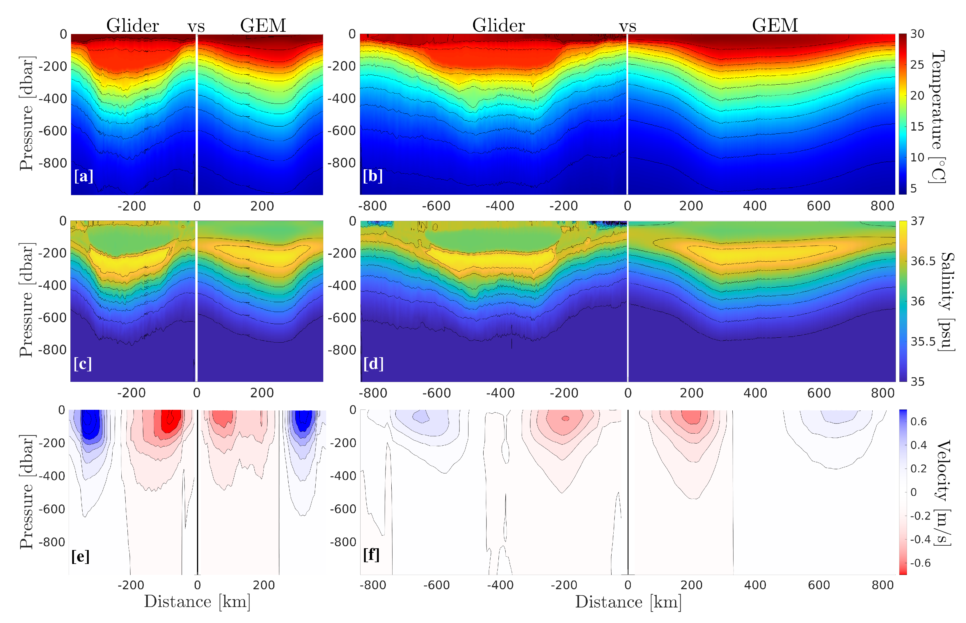
Figure 6 shows the two glider sections and the GEM-reconstructed sections. Note that the first section (panels a, c, and e) was performed as the glider was navigating towards the drifting eddy, while in the second section (panels b, d, and f), the glider and the eddy were moving in the same direction. This results in an under (over) estimation of distances and an over (under) estimation of velocity in the first (second) glider section. This bias was discussed in detail by Meunier et al. [27] and a correction method was proposed by Meunier et al. [30]. However, for validation of the GEM fields, we chose to use the uncorrected glider along track coordinates to keep the analysis as straightforward as possible. For the ease of visualisation, the GEM sections are flipped laterally to appear as a mirror image of the glider sections. In both sections, the LCR is obvious as a downward tilting of the isotherms, both in the glider observations and in the GEM-reconstructed fields. The displacement of the isotherms in the GEM sections is in good agreement with the glider observations up to the 25 °C isotherm. However, the homogeneity of temperature in the upper part of the eddy’s core (thermostat) is not faithfully reproduced by the GEM method, which exhibits a slightly more stratified structure. Note that LCR Poseidon was an uncommon LCR with an exceptionally thick thermostat [27,30], so we hypothesize that this difference is, in part, related to the exceptional nature of Poseidon. The salinity sections, on the other hand, are not subject to this bias, and the double core structure, consisting of a salinity maximum between 200 and 350 m, and a homogeneous salinity minimum above, is well reproduced by the GEM reconstruction. Note that, in both sections, the GEM-reconstructed eddy is slightly smoother, as expected from the methods, which essentially captures the geostrophic, or slow structure of the flow [22]. It should be pointed out that the smoothing of thermohaline gradient has little effect on the geostrophic velocity difference between glider and GEM-derived fields. Indeed, the low-pass filtering required to compute geostrophic velocity from glider observation, removes high wavenumber variability and tends to smooth out gradients, whatever the glider’s original resolution. In other words, the small scale variability that the GEM method is unable to capture has to be removed from the glider data anyway. The vertical sections of geostrophic velocity are shown in panels (e) and (f). In both sections, the agreement between the GEM-reconstructed and the glider sections is evident, both in the spatial patterns and in the magnitude of the velocity.
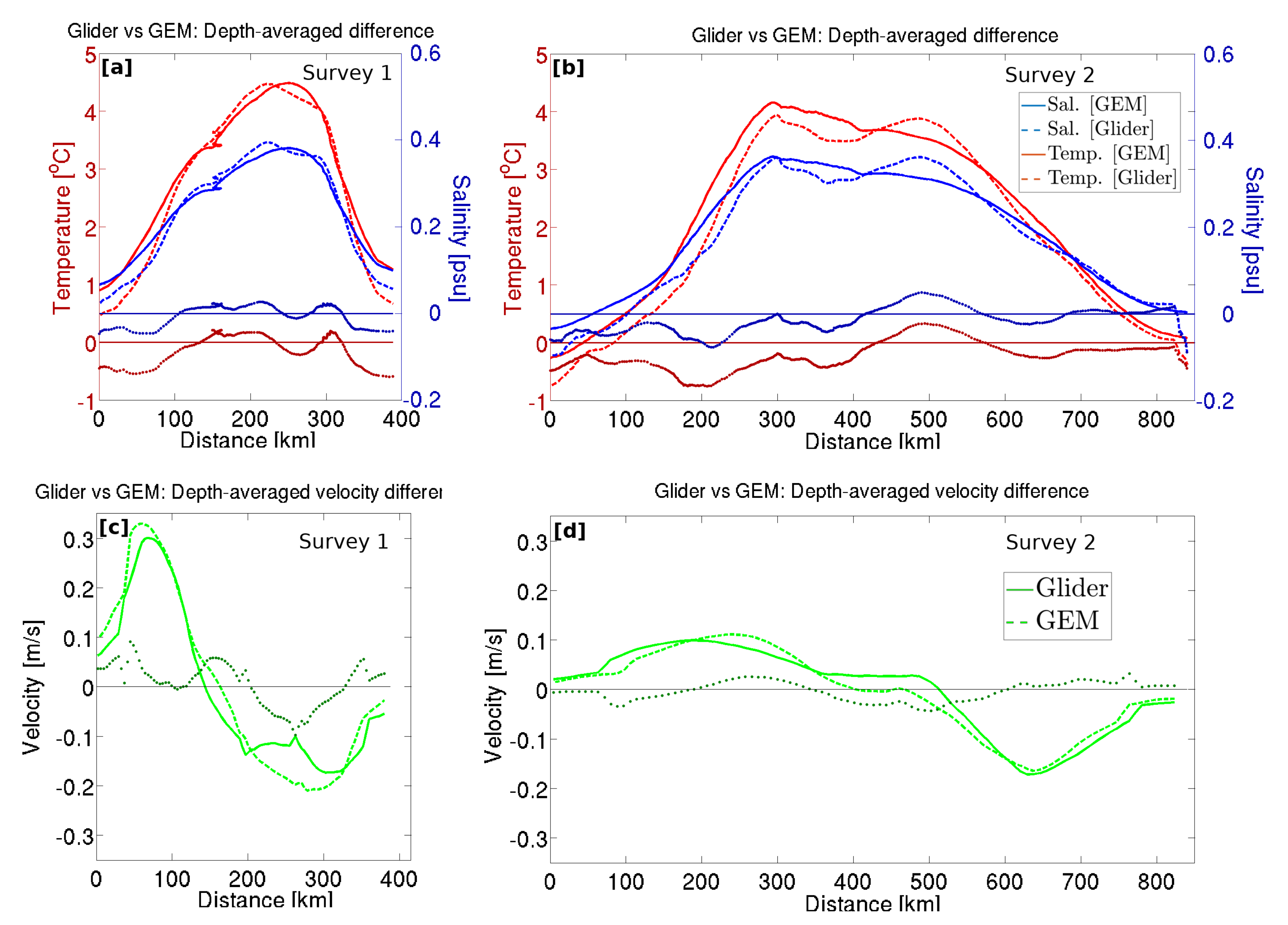
Although the detailed vertical structure of LCRs is of interest, knowledge of the vertical structure of ocean eddies is particularly crucial for the computation of their heat content and transport, which rely on depth-integrated temperature anomaly. Depth-averaged temperature and salinity anomalies, as well as the depth-averaged geostrophic velocity, are shown in Figure 7. In both cross-sections, the glider observation and the GEM-reconstruction are in striking agreement, with a coefficient of determination ( R 2 ) ranging between 0.91 and 0.94, meaning that the GEM method captures over 90 % of the depth averaged velocity, temperature anomaly, and salinity anomaly variance. In particular, one should note that the lateral gradients of depth-averaged variables do not suffer from the over-smoothing that was discernible in the detailed vertical sections. The GEM thus appears to be particularly well-suited to compute integrated variables, such as heat and salt content, or kinetic and available potential energy.

5. The 3D Structure of an Average LCR

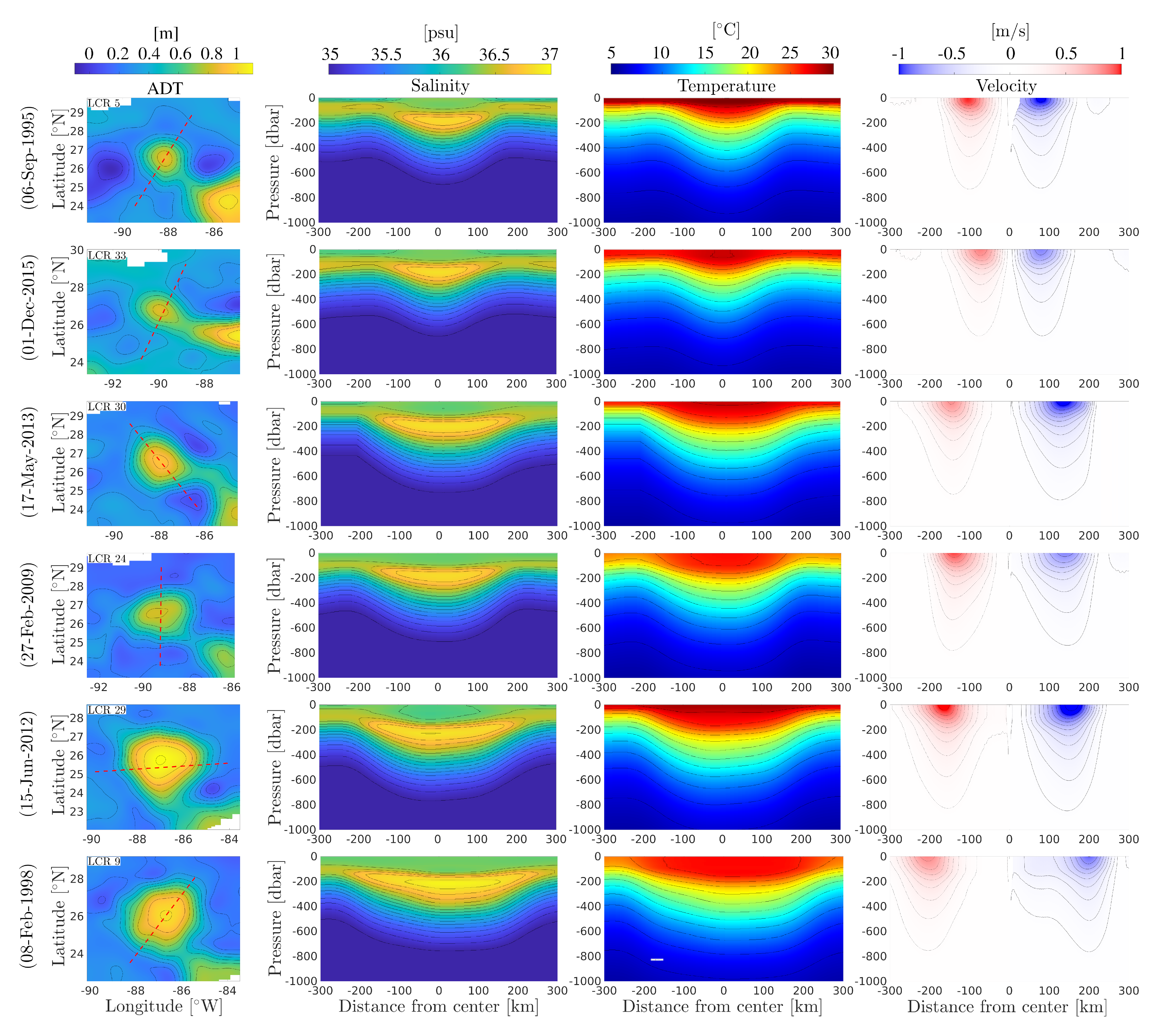
The 3D reconstruction method was applied to 40 LCRs that detached between 1993 and 2021. Cross-sections of salinity, temperature, and cyclogeostrophic velocity are shown in Figure 8 for 6 selected examples. Maps of ADT 5 days after detachment along with the virtual transect trajectories are shown in the left-hand-side panels. These examples were chosen to represent small, average, and large LCRs in spring/summer conditions and in fall/winter conditions. The reconstructed fields capture well the typical LCR structure, which is characterized by a double core salinity structure, consisting of a fresh anomaly in the top 100 to 150 m, lying over a salty anomaly between 150–200 m and 300 m. The thick homogeneous warm anomaly is also evident between the surface and 200 m, and the isotherms are doming downward throughout the water column. In spring/summer conditions, a shallow thermocline lies over the main LCR structure, while in fall/winter conditions, the mixed layer extends down to the base of the thermostat, and is deeper in the LCR than at its periphery.
Geostrophic velocity was computed using the thermal wind relations, using H = 2000 dbar as the level of no motion:
u g ( x , y , z , t ) = g ρ 0 f H 0 k × ρ ( x , y , z , t ) d z ,
where g is the gravity acceleration, ρ 0 is a reference density, f is the Coriolis frequency, is the horizontal gradient operator, k is the vertical unit vector, and ρ is in situ density.
Note that the reference can equally be taken as the surface geostrophic velocity inferred from satellite altimetry, yielding exactly similar results since the GEMs were computed assuming that the geopotential is flat at 2000 dbar.
The velocity fields have maxima ranging between 0.6 and 1 m s 1 and exhibit intense vertical shear in subsurface, with the velocity dropping by ≈70% in the top 300 m.
Although the statistical properties of LCRs presented in this work (
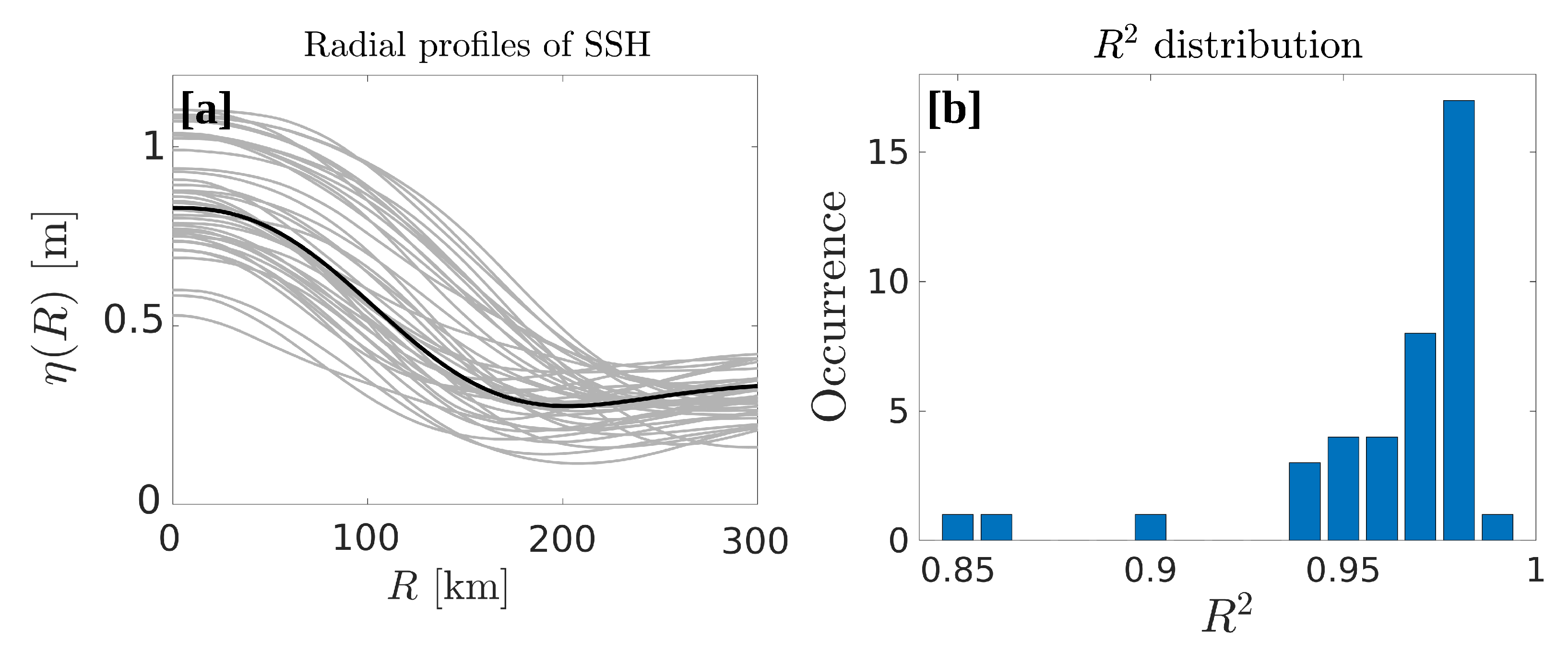
Section 6) are computed using individual GEM reconstructions, it is of interest to determine the average structure of an LCR. To do so, we defined a typical surface signature of LCRs (radial ADT profile) and then used the GEM’s transfer functions to reconstruct the vertical thermohaline structure. Each radial ADT profile was fitted to Zhang et al.’s [35] universal stream function, defined as:
ψ ( r ) = ψ 0 + ψ m ( 1 r ˜ 2 ) e r ˜ 2 ,
r ˜ = r L ,
where ψ ( r ) is the surface stream function, r ˜ is the non-dimensional radial coordinate and L is the radial length scale. ψ 0 is the background stream function value outside the eddy, and ψ m is the amplitude parameter which is equal to the maximum value at the centre of the eddy. In the geostrophic framework considered here, ψ is simply proportional to ADT ( ψ = g f ADT ). For each radial profile of ADT, the parameters η 0 , η m , and L are determined using least-square fitting. Figure 9a shows the mean profiles of each of the 40 LCRs (gray lines), along with the universal stream function computed using the average parameters of each least-square fit (black line). Figure 9b shows the distribution of the coefficient of determination R 2 between the observed and the fitted profiles. R 2 is a measure of the variance fraction that is reproduced by the analytical stream function. The universal stream function appears to faithfully represent LCRs surface signature, with 37 eddies out of 40 having a coefficient of determination superior to 0.95.
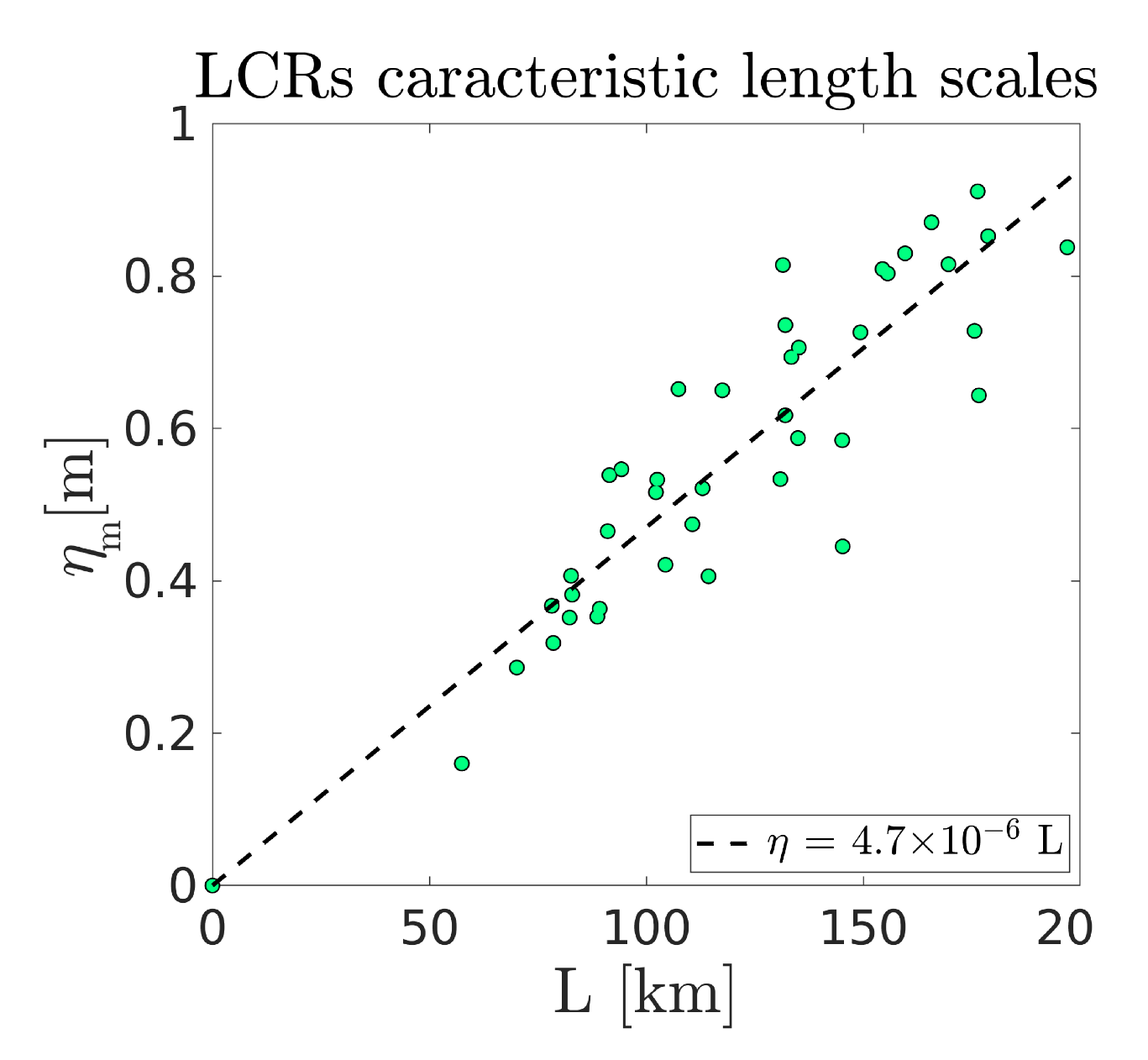
Figure 10 shows values of the ADT anomaly η m against the radial length scale L. In agreement with Figure 5c, the amplitude of the sea surface height deviation in the LCR’s core appears to be approximately proportional to the radial length scale. The parameters chosen for the reference ADT profile are the average of each fitted values, which naturally fall on the linear trend line of Figure 10.
The vertical temperature and salinity fields were then built using the yearly-averaged GEM, and are shown in Figure 11. As in the selected individual examples of 
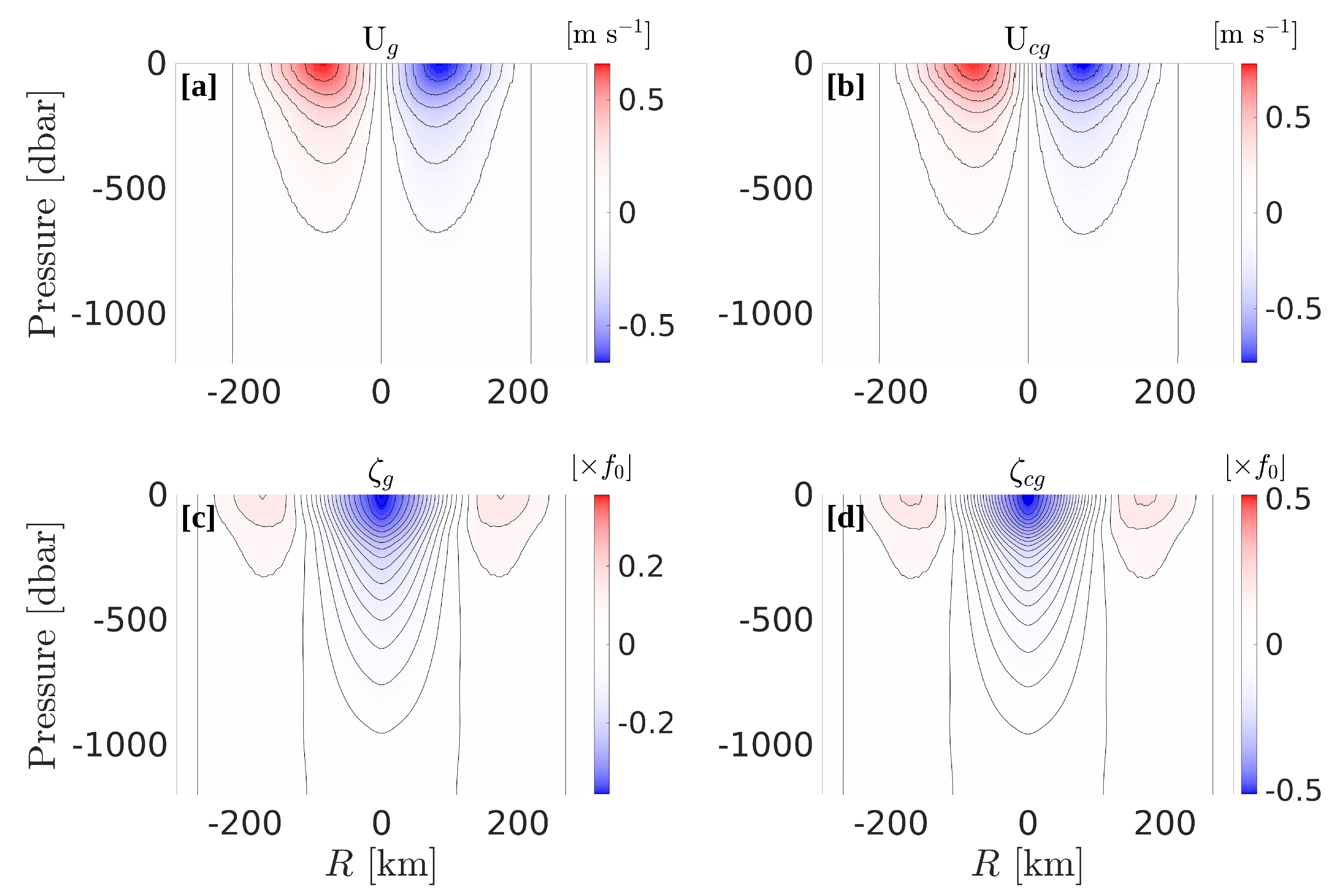
Figure 8, the downward doming of the isotherms towards the eddy’s center is evident, along with a slight decrease in stratification in the eddy’s upper core. The salinity section exhibits the SUW salinity maximum signature near 200 m, and fresher water above. The geostrophic velocity vertical structure (Figure 12a) exhibits well defined velocity maxima of about 0.63 m s 1 , with vertical shear reaching 1.5 × 10 3 s 1 in the top 200 m.
Cyclogeostrophic velocity was also computed for the reference LCR, following Holton [36]. It is the solution of the gradient–wind balance and reads:
u c g ( r , z ) = f r 2 ± f 2 r 2 4 + f r u g ( r , z ) .
Note that for the computation of the mean LCR’s characteristics, the Coriolis frequency is chosen to be constant (Beta plane) and equal to its value at the average eddy-separation latitude. The vertical section of cyclogeostrophic velocity is shown in Figure 12b. Maximum velocity is increased with values reaching 0.76 m s 1 . As expected, the impact of including the centrifugal force in the balance has more impacts in the vicinity of the rotation axis, and the mean velocity increase is of ≈20 % between the velocity maxima and the rotation axis. Relative vorticity was computed both from the geostrophic and cyclogeostrophic velocities. In cylindrical coordinates, it is defined as:
ζ ( r , z ) = 1 r ( r u ϕ ) r ,
where u ϕ is the azimuthal velocity. The LCR’s relative vorticity signature consists in a bowl of negative relative vorticity and is discernible down to 1000 dbar. It is enclosed within a crown of positive relative vorticity at the eddy’s periphery, with a more modest depth extent (≈300 m). As for the azimuthal velocity, cyclogeostrophic vorticity is more intense than geostrophic vorticity, with maximum normalized values reaching 0.51 × f 0 , and 0.35 × f 0 , respectively.
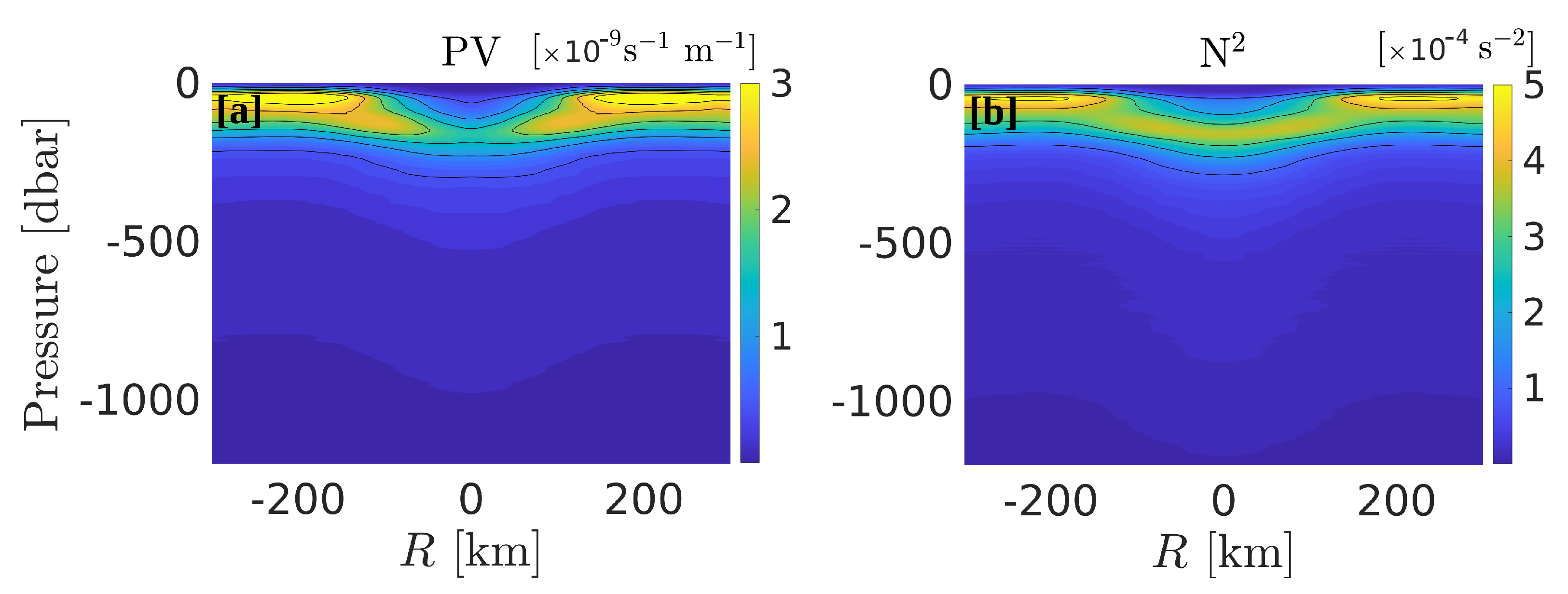
A section of Ertel’s potential vorticity (PV) is shown in Figure 13a. In cylindrical coordinates, PV is defined as:
q ( r , z ) = 1 g ( f + ζ ) N 2 u ϕ z σ r ,
where N 2 is the buoyancy frequency, defines as N 2 = g σ σ z . The LCR is obvious as a bowl of extremely low PV in the top 200 m, deflecting the pycnocline downward. Examination of the vertical structure of the buoyancy frequency (Figure 13b) reveals very similar patterns, suggesting that PV is mostly influenced by the LCR’s stratification.
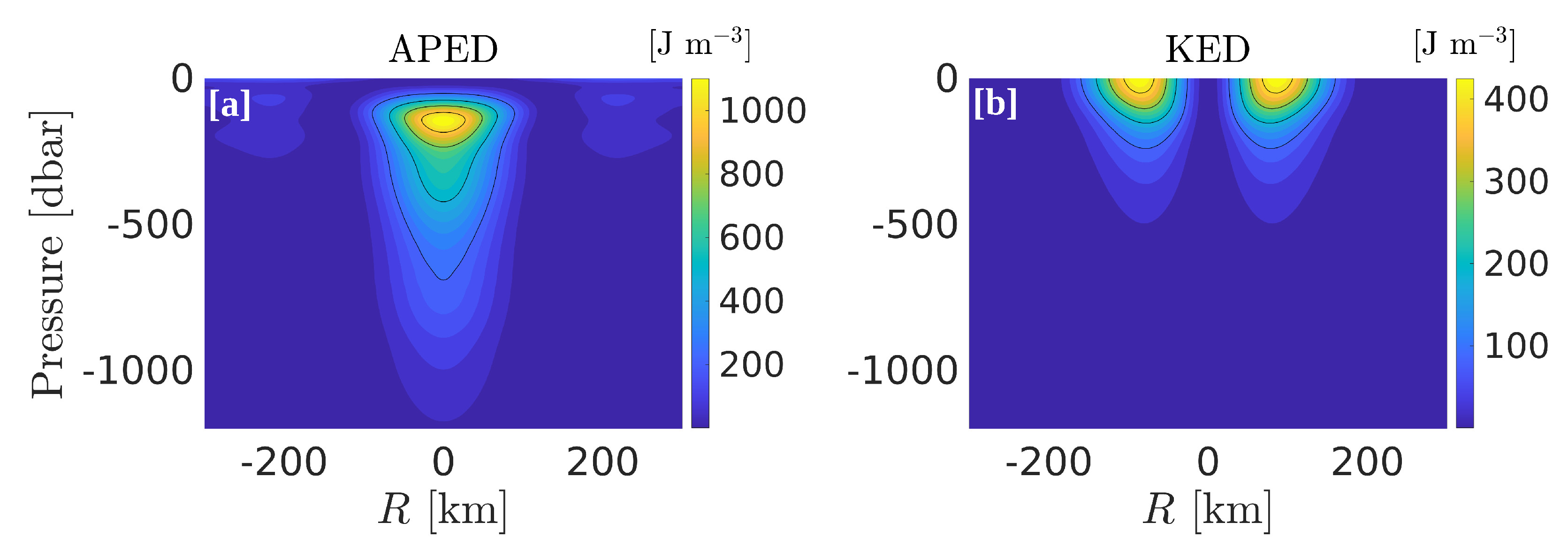
To conclude this description of the vertical structure of an average LCR, the distribution of mechanical energy density is shown in Figure 14. Kinetic energy density (KED) and available potential energy density (APED) are defined following Holliday and McIntyre [37]:
E k ( r , z ) = 1 2 ρ u ϕ 2 ( r , z ) ,
E p ( r , z ) = g 0 δ δ ˜ ( r , z ) d ρ ¯ d z ( z δ ˜ ( r , z ) ) d δ ˜ ,
ρ ¯ ( z ) is the reference density profile, which is defined as the minimum potential energy profile in the GoM, and obtained by adiabatically sorting all available density measurements, and δ is the isopycnal displacement. The LCR’s vertical structure consists of a subsurface bowl of intense APED intensified between 150 and 200 m, where isopycnal displacement and density anomaly are maximum. There is no surface signature, while APED anomaly is evident down to 1200 m. KED exhibits significantly smaller values than APED, and is maximum at the periphery of the eddy, while APED is maximum in the core. When integrated over the whole eddy’s volume, we find a ratio of KE/APE ≈ 1/3, so that energy partition is strongly skewed.

6. Heat, Salt, and Energy Statistical Properties

One particularly important application of this three-dimensional individual eddy reconstruction method, is to achieve a statistical representation of LCRs properties, and of their impacts on the GoM’s heat, salt, and energy budget. The heat and salt content anomalies associated with each LCR with a boundary C enclosing a surface S are defined as:
H = S H 0 ρ 0 C p δ T d z d S
S = S H 0 δ S d z d S ,
where d S is a surface element, C p is the specific heat of sea water, ρ 0 is the mean density, δ T is the temperature anomaly, defined as the difference between the temperature T ( x , y , z , t ) and the GoM’s mean profile T ¯ ( z ) , and δ S is salinity anomaly (in kg m 3 
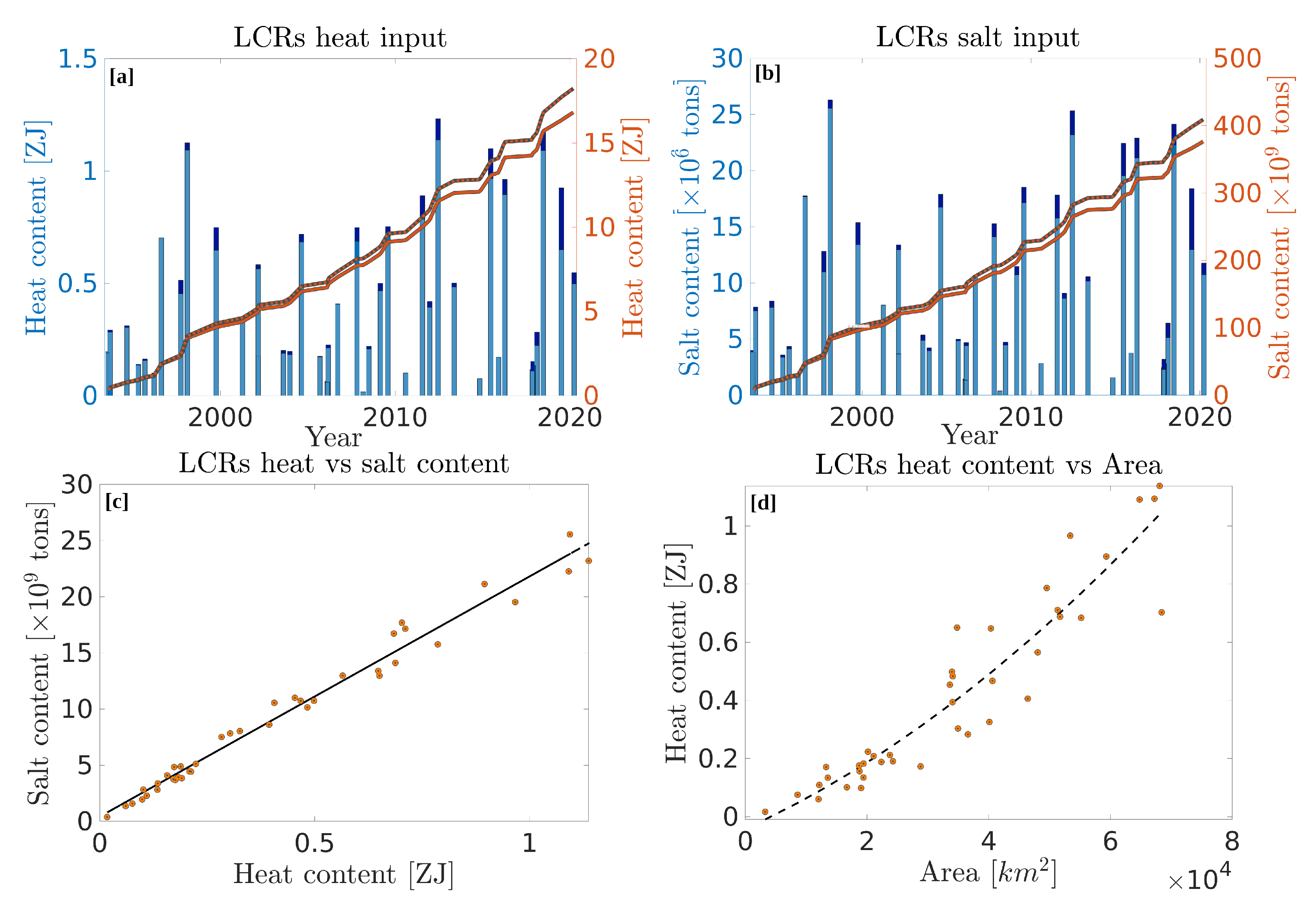
), defined using the same procedure as for temperature anomaly. Heat and salt contents of the 40 detected eddies are shown on the bar plots of Figure 15a,b for two different eddy boundary criteria (maximum velocity contour and last closed ADT contour) and are compared against each other on Figure 15c. The average heat content of an LCR is of 0.42 and 0.46 ZJ for the maximum velocity contour and the last closed contour boundary criteria, respectively, while the average salt content is of 9.43 and 10.24 billion tons. Heat and salt are extremely variable from one eddy to the other, with a range spanning nearly 2 orders of magnitude ((0.017–1.14) ZJ for heat and (0.38–25.5) billion tons for salt). There is a solid proportionality relationship ( R 2 = 0.98) between heat and salt contents (Figure 15c), in agreement with Meunier et al. [20]. The cumulative heat and salt input into the GoM were also computed between 1993 and 2022, and are shown as the orange lines in Figure 15a,b. Despite the large variability of LCRs heat and salt contents, and the lack of periodicity in eddy detachment events, the cumulative heat input grows nearly linearly with time, with a growth rate of 0.60 ZJ per year for heat and 13.5 billion tons per year for salt (coefficient of determination R 2 = 0.99 for both heat and salt linear fits). It is also interesting to note that the individual heat contents of LCRs do not grow linearly with their surface area, but rather quadratically (Figure 15d), which might be attributed to the fact that larger eddies also have larger maximum SSH anomalies, hence, not only larger areas, but also larger heat content anomalies per unit area.
The kinetic and potential energy carried by the LCRs were also estimated. Kinetic and available potential energy ( E k and E p , respectively) are defined as the volume integral of KED and APED (defined in Equations (7) and (8), respectively):
E k = S H 0 E k d z d S ,
E p = S H 0 E p d z d S
Similar to the heat and salt contents discussed above, the total energy carried by each individual LCR is shown in the bar plot of Figure 16a. The cumulative energy is plotted for KE, APE, and total mechanical energy (TE = KE + APE), while the individual energy contents (bar plot) is only shown for TE, for the sake of clarity. Total mechanical energy has an average of 10.0 (10.9) PJ per eddy when defining the eddies boundaries as the maximum velocity contour (last closed contour). They also exhibit a wide range of values with nearly two orders of magnitudes between the less energetic and the more energetic eddies ((0.15–36.6) PJ). On average, APE is 3.8 times larger than KE. This bias in the energy partition is particularly evident in Figure 16b, which shows KE against APE for each detected LCR. The black line represent equipartition (Burger number unity). Although APE dominates over KE in all LCRs, the ratio between KE and APE (Burger number) decreases as the LCRs total energy increases: large eddies have very small Burger numbers, while smaller eddies can get closer to energy equipartition. The growth of cumulative energy is also nearly linear, with values of 2.95 and 11.2 PJ per year for KE and APE, respectively ( R 2 = 0.99 for KE and 0.97 for APE).
It is of interest to put these large numbers back into the context of temperature, salinity and energy balance in the Gulf of Mexico. Attempting a full closed budget of the GoM is beyond the scope of this paper, but we can compute a number of meaningful quantities that highlight the importance of LCRs in the GoM’s dynamics.
For instance, it is of interest to estimate the residual net surface heat flux that would be necessary to balance the 0.60 ZJ per year heat input of LCRs into the GoM. Under the assumption that the heat carried by each LCR will eventually totally mix with the GoM water, the necessary residual heat fluxes can be simply estimated by dividing this heat growth rate by the surface of the GoM ( A GOM = 1.58 millions km 2 ), or equivalently, since the heat growth rate can be considered as linear, by dividing the total heat input of the 40 detected eddies by the time interval ( τ = 29 years) multiplied by the surface of the GoM [20]:
Q b = i = 1 40 H i τ A GOM .
Here, we find that a yearly net residual heat flux of −13 W m 2 is necessary to compensate LCRs heat input into the GoM. This value is very close from that of Meunier et al. [20] (14 W m 2 ), using a simple linear relationship between SSH and local heat content. Because the literature reveals a wide range of residual net surface heat flux estimates (between −24 and +46 W m 2 [38,39,40]), knowing the value necessary to balance LCRs heat could be helpful to calibrate heat flux products.
A similar argument can be used to estimate the necessary fresh water input in the GoM to balance the 13.5 billion tons of salt excess per year carried by LCRs. Following Meunier et al. [20], the necessary flux of fresh water input is:
F b = i = 1 40 S i τ S ¯ GOM ,
where S ¯ GOM is the average salinity of the GoM. Here, we find that a fresh water flux of 12,000 m 3 s 1 would be necessary for the GoM’s mean salinity to remain constant despite the LCRs salt input. This value is also very close from Meunier et al.’s [20] estimate (12,700 m 3 s 1 ) using a simple linear relationship between SSH and local salt content. It should be pointed out that these values are closely matching Morey et al.’s [41] recent estimates of the Mississippi river outflow (13,000 m 3 s 1 ), suggesting that the opposing effects of LCRs and the Mississippi river on the GoM’s salinity approximately cancel each other.
We can similarly estimate the energy dissipation rate that would be necessary to dissipate LCRs energy:
ϵ b = i = 1 40 E i τ ρ 0 V ,
where V is the volume of water in which we expect energy to be dissipated. We explore three different hypotheses: (a) energy is homogeneously dissipated within the whole GoM’s volume; (b) energy is dissipated within the top 1000 m; and (c) energy is dissipated within the top 500 m. The necessary dissipation rate is respectively of 1.8, 4.5, and 9.0 × 10 10 W kg 1 . These values are lower than direct microstructure measurements in the vicinity of LCRs by Molodstov et al.’s [42] (( 10 9 10 8 ) W kg 1 ), but are consistent with their GoM’s background values ( 10 10 10 9 ) W kg 1 , as well as Whalen et al.’s [43] estimates between 250 and 500 m, using fine-scale strain parameterization (≈5 × 10 10 W kg 1 ).
To emphasize the need for the compensation of heat, salt and energy excesses input to the GoM through LCR detachment, it is of interest to investigate what would happen in the absence of surface heat fluxes, fresh water influx, and energy dissipation. To do so, we computed the temperature, salinity, SSH, and energy density rise that would occur if LCRs detachment was not balanced by any process. As for our energy dissipation estimates, we propose three scenarios: the heat, salt, and energy excess are homogeneously redistributed into: (a) the whole GoM volume; (b) the top 2000 m; and (c) the top 1000 m. For each individual LCR, the mean temperature, salinity, and energy density rises read:
Δ T i = H i ρ 0 C p V
Δ S i = S i V
Δ E i = E i V
where V represents weather the full water volume of the GoM, or that of the top 2000 or 1000 m. The equivalent sea level rise is computed as the difference between the steric height associated with the mean GoM temperature and salinity ( T ¯ and S ¯ ), and the steric height associated with the hypothetical increased temperature and salinity ( T ¯ + Δ T and S ¯ + Δ S 
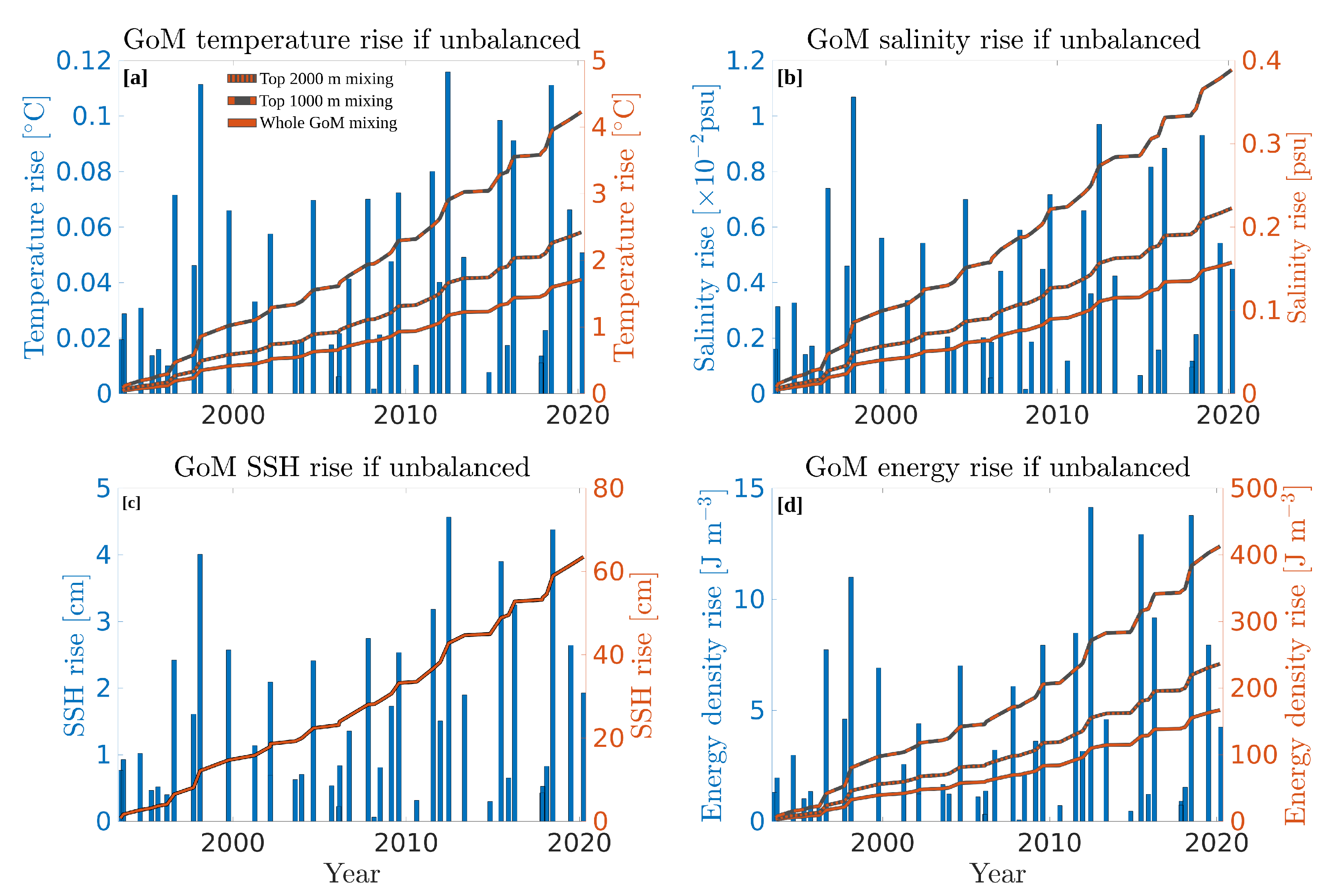
). The hypothetical (unbalanced) impacts of each individual LCR, as well as their cumulative impacts over time on temperature, salinity, SSH, and energy density are shown in Figure 17. For the sake of clarity, only hypothesis (a) (redistribution of tracers over the entire GoM volume) is shown in the bar graphs, while the three scenarios are plotted for the cumulative effects. Because of the heterogeneity of LCRs heat, salt, and energy content, the hypothetical unbalanced response of the GoM to individual eddies is highly variable. On average, mixing of a mean LCR into the whole GoM, the top 2000 m, or the top 1000 m would result in a rise of 0.04, 0.06, and 0.10 °C of the GoM’s mean temperature, respectively (Figure 17a). For the largest LCRs, these values reach up to 0.12, 0.16, and 0.28 °C. Looking at the cumulative effects of LCRs, between 1993 and 2021, if unbalanced by surface heat fluxes, the GoM’s mean temperature would have risen by 1.71, 2.42, and 4.23 °C in the whole GoM, top 2000 m, and top 1000 m mixing scenarios, respectively.
Using similar arguments, in the absence of fresh water input, the average salinity of the GoM would rise by 0.0039 psu after mixing an average LCR within the whole GoM volume (0.0056 and 0.010 psu if the LCRs mixes with the GoM’s top 2000 and 1000 m water mass), while the largest individual LCRs could yield a mean salinity increase of 0.011, 0.015, and 0.026 for in the three scenarios (Figure 17b). If unbalanced, the salt excess of LCRs would have induced a salinity rise of 0.16, 0.22, or 0.39 psu depending on the mixing depth, between 1993 and 2021.
Although the halosteric effect associated with the salinity increase would partially compensate the thermosteric effects due to temperature increase, in the absence of balancing processes, LCRs would have caused a sea level rise of 63 cm over the 29 year study period (Figure 17c).
If energy was not dissipated, energy density in the GoM would have increased by 167, 236, or 413 J m 3 , depending on the scenario. As an illustrative reference, these levels of energy density would be equivalent to the kinetic energy density of currents of 0.57, 0.68, and 0.89 m s 1 over the full water column, top 2000, and top 1000 m of the entire GoM. Obviously, such temperature, salinity, SSH, and energy density increase is not observed, and these hypothetical scenarios are presented to highlight both the crucial importance of LCRs in the GoM’s dynamics and budgets, as well as the evident need to accurately measure the surface heat fluxes and fresh water inputs when modelling a semi-enclosed basin with such important advective fluxes.

7. Conclusions

In this work, we applied the GEM method [21,22] to satellite altimetry data, similarly to Swart et al. [23], Stendardo et al. [31], and Müller et al. [24], to reconstruct the three-dimensional structure of individual LCRs in the GoM.
Although the joint use of the GEM and satellite altimetry to infer heat and salt contents of mesoscale eddies was first proposed by Müller et al. [24], here, we extended the method to the computation of the full three-dimensional velocity, vorticity and energy density structure of mesoscale eddies.
The method was validated using independent glider observations, showing that the GEM-reconstruction was able to represent accurately the vertical structure of temperature, salinity, and geostrophic velocity of LCRs, especially when comparing depth-integrated variables.
The application of this three-dimensional reconstruction procedure allowed the success of two primary goals: 1. determine the typical structure of LCRs by computing their average thermohaline and dynamical structure; 2. estimate statistical properties of LCRs heat, salt, and energy contents, as well as their cumulative effect.
Consistent with previous ship and glider observations of individual LCRs [7,27], the typical LCR is characterized by a warm temperature anomaly with weaker stratification, and a double core salinity structure, with a fresher anomaly near the surface and a high salinity anomaly between 150 and 300 m. Although typical LCRs are large eddies, we found that the gradient–wind balanced velocity was significantly larger than the geostrophic velocity (≈+20% between the rotation axis and the maximum velocity radius), similar to Meunier et al.’s [30] recent observation in LCR Poseidon. This results in an increased relative vorticity, reaching half of the Coriolis frequency, showing that average LCRs (medium size) are significantly non-linear eddies with a Rossby radius of 0.5. The average LCR’s PV structure consists of a bowl of low PV deflecting the main pycnocline’s high PV strip downwards, and is mostly controlled by density stratification. It should be pointed out that the average LCR computed here has a weaker PV anomaly, with a lesser vertical extension, than the recent observations of Meunier et al. [30] of LCR Poseidon. We stress this is related to the exceptionally thick thermostadt observed in Poseidon, while the work is focused on describing an average LCR. However, the GEM-reconstructed energy density structure of the mean LCR exhibited a similar pattern than Meunier et al.’s [30] direct observations, with a clear dominance of APE over KE. However, it should be pointed out that the smoothing of the thermostat by the GEM reconstruction, as compared to the glider observations (Section 4) might slightly bias our estimates of APE and KE. For the two available glider sections, we found that the GEM-reconstructed eddy’s APE was about 10% smaller than the glider-measured eddy. Similarly, KE was reduced by about 9% and potential enstrophy (volume integral of the squared PV) by 12.5 and 22% depending on the glider section.
By detecting and studying a large number of LCRs (40), we were able to assess statistical properties of their heat, salt, and energy contents, as well as their cumulative effects on the GoM. One particularly striking characteristic of LCRs is their heterogeneity: the ratio of standard deviation over the mean value for LCRs heat and salt contents is of 0.76 and 0.73, respectively. They, thus, have a very variable impact on heat and salt input into the GoM: the cumulative effect of the 20% largest eddies contribute to half of the total heat and salt input between 1993 and 2021.
As an illustration of the importance of LCRs to the heat, salt, and energy inputs of LCRs in the GoM, we computed the temperature, salinity, SSH, and energy density rises that would occur in the absence of balancing processes and showed that, in the hypothesis that LCRs would eventually mix homogeneously within the entire GoM’s volume, the mean temperature and salinity would have increased by nearly 2 °C and 0.15 psu, respectively, between 1993 and 2021, causing a ≈60 cm sea level rise. Over the same period, the energy density would have increased to a level equivalent to mean barotropic currents of nearly 0.6 m s 1 over the whole GoM. Another way to appreciate these numbers is to estimate the time it would take for the GoM’s mean temperature and salinity (7.7 °C and 35.2 psu for the top 2000 m for the 2010–2020 period) to reach Caribbean values (9.9 °C and 35.36 psu for the same depth range and period). Here, we find that if LCRs heat and salt inputs were not balanced, it would only take 25 years for the GoM to have pure SUW properties. Another particularly striking result is that one single unbalanced large LCR would be able to increase the GoM’s mean temperature by over 0.1 °C, yielding a sea level rise of nearly 5 cm.
Obviously, the heat, salt, and energy budgets in the Gulf of Mexico do not fall down to an inevitable accumulation of LCRs input, and the numbers presented in the last paragraph are only intended to emphasize the large impact of LCRs, as well as the need for compensating processes. Because the GoM is a semi-enclosed basin, whose entrance (the Yucatan channel) and exit (the Florida strait) are directly connected by the Loop Current, a straightforward model for volume-integrated budgets is that the heat input of LCRs can be balanced by an outward advective heat flux and surface heat fluxes, their salt input by an outward advective salt flux and fresh water input, and their energy by an outward advective energy flux, energy dissipation, and wind stress work. Because the Florida strait is shallower than the Yucatan channel, and the warm and salty anomaly associated with the SUW reach deeper depths than the strait’s depth [44,45], the only possible advective heat flux to partially compensate for the LCRs input would take place in the deeper Yucatan channel. However, Bunge et al. [46] and Candela et al. [47] showed that, despite bursts of outflow through the deep Yucatan channel, mostly related to mass conservation as the Loop Current grows in the GoM, the long term average deep transport is near-zero. Rivas et al. [48] estimated that the advective heat and salt flux through the Yucatan channel were of −30 GW and 1.1 tons per second, respectively. Here, we find that the 29 year trends in LCR heat and salt input are of 19,100 GW and 427 tons of salt per second, so that the advective heat and salt fluxes through the deep Yucatan channel are several orders of magnitudes too small to balance LCRs. LCRs heat, salt, and energy thus must be entirely compensated by surface heat fluxes, fresh water input (river outflow plus precipitation minus evaporation), and energy dissipation. From this very simple remaining balance, we found that net residual heat fluxes of −13 W m 2 were necessary to keep the GoM’s mean temperature constant, in good agreement with Meunier et al.’s [20] estimate. This number could be useful to calibrate and validate heat flux products in the GoM, as well as regional model configurations.
We also estimated the necessary fresh water input to be of 12,000 m 3 s 1 : 5 % less than Meunier et al.’s [20] estimates, and still closely matching the Mississippi river outflow. Note that a fully closed salinity budget of the GoM should also include evaporation and precipitation, which is expected to be a fresh water loss in the GoM, hence requiring larger river outflows for balance to be reached. However, as mentioned above, the scope of this paper is not to make a full budget analysis, but rather to quantify the impact of LCRs and highlight possible balancing processes. Similarly, an attempt to close the GoM’s energy budget is beyond the scope of this paper, and would require a careful computation of the wind work and of the buoyancy fluxes through Ekman pumping, using the relative wind (wind minus current velocity) [49,50,51]. In fact, energy loss of LCRs through relative wind work and energy transfer from APE to KE through Ekman buoyancy fluxes are to be expected for a mesoscale eddy subject to wind forcing [51], and are currently under investigation. However, our simple scaling of the order of magnitude of an equivalent energy dissipation rate ϵ is in good agreement with values observed in the GoM [42,43].
The results reported here highlight the possibility and the utility to reconstruct the three-dimensional structure of individual mesoscale eddies (as opposed to the computation of one single mean composite eddy [12]) from satellite altimetry and the GEM method. The application of the method used and described in the present paper to other regions of the ocean could help to elucidate the role of coherent mesoscale eddies in basin-scale heat, salt, and energy exchange. However, one should note that the method is not expected to be accurate everywhere in the ocean, since more complex hydrographic conditions may exist and make the computation of a reliable GEM field more difficult. These results also emphasize the crucial role of LCRs in the GoM, and suggests that more research is necessary to elucidate the processes controlling LCRs (and mesoscale coherent eddies in general) mixing and decay processes.

Author Contributions

Conceptualization, T.M.; methodology, T.M. and P.P.-B.; software, T.M.; validation, T.M.; formal analysis, T.M.; investigation, T.M.; resources, A.B.; data curation, T.M.; writing—original draft preparation, T.M.; writing—review and editing, A.B. and P.P.-B.; visualization, T.M.; supervision, T.M., A.B. and P.P.-B.; project administration, A.B.; funding acquisition, A.B. All authors have read and agreed to the published version of the manuscript.

Funding

This work is part of the LC-floats project, funded by the US National Academy of Sciences through the Understanding Gulf Ocean Systems grant 2000010488.

Data Availability Statement

All data used in this study are publicly available. The ARGO data can be retrieved from https://argo.ucsd.edu/ (accessed on 1 July 2022). The absolute dynamic topography data are produced by AVISO, and distributed by Copernicus Marine Service (https://resources.marine.copernicus.eu/ (accessed on 1 July 2022)). Glider data were collected by the GMOG group at CICESE (https://gliders.cicese.mx/ (accessed on 1 July 2022)).

Acknowledgments

The authors are grateful to Enric Pallás-Sanz and Miguel Tenreiro from the GMOG group at CICESE for providing the glider data used for validation of the GEM method.

Conflicts of Interest

To the best of their knowledge, the authors have no conflicts of interest.

References

  1. Olson, D.B.; Evans, R.H. Rings of the Agulhas current. Deep Sea Res. A 1986, 33, 27–42. [Google Scholar] [CrossRef]
  2. Wang, Y.; Beron-Vera, F.J.; Olascoaga, M.J. The life cycle of a coherent Lagrangian Agulhas ring. J. Geophys. Res. Ocean. 2016, 121, 3944–3954. [Google Scholar] [CrossRef]
  3. Richardson, P. Gulf stream rings. In Eddies in Marine Science; Springer: Berlin/Heidelberg, Germany, 1983; pp. 19–45. [Google Scholar]
  4. Liu, Y.; Wilson, C.; Green, M.A.; Hughes, C.W. Gulf Stream Transport and Mixing Processes via Coherent Structure Dynamics. J. Geophys. Res. Ocean. 2018, 123, 3014–3037. [Google Scholar] [CrossRef]
  5. Li, L.; Nowlin, W.D.; Jilan, S. Anticyclonic rings from the Kuroshio in the South China Sea. Deep Sea Res. Part I Oceanogr. Res. 1998, 45, 1469–1482. [Google Scholar] [CrossRef]
  6. Sasaki, Y.N.; Minobe, S. Climatological Mean Features and Interannual to Decadal Variability of Ring Formations in the Kuroshio Extension Region. In Proceedings of the AGU Fall Meeting Abstracts, San Fancisco, CA, USA, 15–19 December 2014; Volume 2014, p. OS41F-07. [Google Scholar]
  7. Elliott, B.A. Anticyclonic Rings in the Gulf of Mexico. J. Phys. Oceanogr. 1982, 12, 1292–1309. [Google Scholar] [CrossRef]
  8. Donohue, K.A.; Watts, D.R.; Hamilton, P.; Leben, R.; Kennelly, M. Loop Current Eddy formation and baroclinic instability. Dyn. Atmos. Ocean. 2016, 76, 195–216. [Google Scholar] [CrossRef]
  9. Beron-Vera, F.J.; Olascoaga, M.J.; Wang, Y.; Triñanes, J.; Pérez-Brunius, P. Enduring Lagrangian coherence of a Loop Current ring assessed using independent observations. Sci. Rep. 2018, 8, 11275. [Google Scholar] [CrossRef]
  10. Andrade-Canto, F.; Karrasch, D.; Beron-Vera, F.J. Genesis, evolution, and apocalypse of Loop Current rings. Phys. Fluids 2020, 32, 116603. [Google Scholar] [CrossRef]
  11. Chelton, D.B.; Schlax, M.G.; Samelson, R.M. Global observations of nonlinear mesoscale eddies. Prog. Oceanogr. 2011, 91, 167–216. [Google Scholar] [CrossRef]
  12. Chaigneau, A.; Le Texier, M.; Eldin, G.; Grados, C.; Pizarro, O. Vertical structure of mesoscale eddies in the eastern South Pacific Ocean: A composite analysis from altimetry and Argo profiling floats. J. Geophys. Res. Ocean. 2011, 116, C11025. [Google Scholar] [CrossRef]
  13. Yang, G.; Wang, F.; Li, Y.; Lin, P. Mesoscale eddies in the northwestern subtropical Pacific Ocean: Statistical characteristics and three-dimensional structures. J. Geophys. Res. Ocean. 2013, 118, 1906–1925. [Google Scholar] [CrossRef]
  14. Yang, G.; Yu, W.; Yuan, Y.; Zhao, X.; Wang, F.; Chen, G.; Liu, L.; Duan, Y. Characteristics, vertical structures, and heat/salt transports of mesoscale eddies in the southeastern tropical Indian Ocean. J. Geophys. Res. Ocean. 2015, 120, 6733–6750. [Google Scholar] [CrossRef]
  15. Keppler, L.; Cravatte, S.; Chaigneau, A.; Pegliasco, C.; Gourdeau, L.; Singh, A. Observed Characteristics and Vertical Structure of Mesoscale Eddies in the Southwest Tropical Pacific. J. Geophys. Res. Ocean. 2018, 123, 2731–2756. [Google Scholar] [CrossRef]
  16. He, Q.; Zhan, H.; Cai, S.; He, Y.; Huang, G.; Zhan, W. A New Assessment of Mesoscale Eddies in the South China Sea: Surface Features, Three-Dimensional Structures, and Thermohaline Transports. J. Geophys. Res. Ocean. 2018, 123, 4906–4929. [Google Scholar] [CrossRef]
  17. de Marez, C.; L’Hégaret, P.; Morvan, M.; Carton, X. On the 3D structure of eddies in the Arabian Sea. Deep Sea Res. Part I Oceanogr. Res. 2019, 150, 103057. [Google Scholar] [CrossRef]
  18. Laxenaire, R.; Speich, S.; Stegner, A. Evolution of the Thermohaline Structure of One Agulhas Ring Reconstructed from Satellite Altimetry and Argo Floats. J. Geophys. Res. Ocean. 2019, 124, 8969–9003. [Google Scholar] [CrossRef]
  19. Sandalyuk, N.V.; Bosse, A.; Belonenko, T.V. The 3-D Structure of Mesoscale Eddies in the Lofoten Basin of the Norwegian Sea: A Composite Analysis From Altimetry and In Situ Data. J. Geophys. Res. Ocean. 2020, 125, e16331. [Google Scholar] [CrossRef]
  20. Meunier, T.; Sheinbaum, J.; Pallàs-Sanz, E.; Tenreiro, M.; Ochoa, J.; Ruiz-Angulo, A.; Carton, X.; de Marez, C. Heat Content Anomaly and Decay of Warm-Core Rings: The Case of the Gulf of Mexico. Geophys. Res. Lett. 2020, 47, e85600. [Google Scholar] [CrossRef]
  21. Watts, D.R.; Sun, C.; Rintoul, S. A Two-Dimensional Gravest Empirical Mode Determined from Hydrographic Observations in the Subantarctic Front. J. Phys. Oceanogr. 2001, 31, 2186–2209. [Google Scholar] [CrossRef]
  22. Sun, C.; Watts, D.R. A circumpolar gravest empirical mode for the Southern Ocean hydrography. J. Geophys. Res. Ocean. 2001, 106, 2833–2855. [Google Scholar] [CrossRef]
  23. Swart, S.; Speich, S.; Ansorge, I.J.; Lutjeharms, J.R.E. An altimetry-based gravest empirical mode south of Africa: 1. Development and validation. J. Geophys. Res. Ocean. 2010, 115, C03002. [Google Scholar] [CrossRef]
  24. Müller, V.; Kieke, D.; Myers, P.G.; Pennelly, C.; Steinfeldt, R.; Stendardo, I. Heat and Freshwater Transport by Mesoscale Eddies in the Southern Subpolar North Atlantic. J. Geophys. Res. Ocean. 2019, 124, 5565–5585. [Google Scholar] [CrossRef]
  25. Hamilton, P.; Leben, R.; Bower, A.; Furey, H.; Pérez-Brunius, P. Hydrography of the Gulf of Mexico Using Autonomous Floats. J. Phys. Oceanogr. 2018, 48, 773–794. [Google Scholar] [CrossRef]
  26. Portela, E.; Tenreiro, M.; Pallàs-Sanz, E.; Meunier, T.; Ruiz-Angulo, A.; Sosa-Gutiérrez, R.; Cusí, S. Hydrography of the Central and Western Gulf of Mexico. J. Geophys. Res. Ocean. 2018, 123, 5134–5149. [Google Scholar] [CrossRef]
  27. Meunier, T.; Pallás-Sanz, E.; Tenreiro, M.; Portela, E.; Ochoa, J.; Ruiz-Angulo, A.; Cusí, S. The vertical structure of a Loop Current Eddy. J. Geophys. Res. Ocean. 2018, 123, 6070–6090. [Google Scholar] [CrossRef]
  28. Meunier, T.; Tenreiro, M.; Pallàs-Sanz, E.; Ochoa, J.; Ruiz-Angulo, A.; Portela, E.; Cusí, S.; Damien, P.; Carton, X. Intrathermocline Eddies Embedded Within an Anticyclonic Vortex Ring. Geophys. Res. Lett. 2018, 45, 7624–7633. [Google Scholar] [CrossRef]
  29. Meunier, T.; Pallàs Sanz, E.; Tenreiro, M.; Ochoa, J.; Ruiz Angulo, A.; Buckingham, C. Observations of Layering under a Warm-Core Ring in the Gulf of Mexico. J. Phys. Oceanogr. 2019, 49, 3145–3162. [Google Scholar] [CrossRef]
  30. Meunier, T.; Pallás Sanz, E.; de Marez, C.; Pérez, J.; Tenreiro, M.; Ruiz Angulo, A.; Bower, A. The Dynamical Structure of a Warm Core Ring as Inferred from Glider Observations and Along-Track Altimetry. Remote Sens. 2021, 13, 2456. [Google Scholar] [CrossRef]
  31. Stendardo, I.; Rhein, M.; Hollmann, R. A high resolution salinity time series 1993–2012 in the North Atlantic from Argo and Altimeter data. J. Geophys. Res. Ocean. 2016, 121, 2523–2551. [Google Scholar] [CrossRef]
  32. Leben, R.R. Altimeter-derived loop current metrics. Wash. Am. Geophys. Union Geophys. Monogr. Ser. 2005, 161, 181–201. [Google Scholar] [CrossRef] [Green Version]
  33. Isern-Fontanet, J.; Font, J.; García-Ladona, E.; Emelianov, M.; Millot, C.; Taupier-Letage, I. Spatial structure of anticyclonic eddies in the Algerian basin (Mediterranean Sea) analyzed using the Okubo Weiss parameter. Deep Sea Res. Part II Top. Stud. Oceanogr. 2004, 51, 3009–3028. [Google Scholar] [CrossRef]
  34. Rudnick, D.L.; Johnston, T.M.S.; Sherman, J.T. High-frequency internal waves near the Luzon Strait observed by underwater gliders. J. Geophys. Res. Ocean. 2013, 118, 774–784. [Google Scholar] [CrossRef]
  35. Zhang, Z.; Zhang, Y.; Wang, W.; Huang, R.X. Universal structure of mesoscale eddies in the ocean. Geophys. Res. Lett. 2013, 40, 3677–3681. [Google Scholar] [CrossRef]
  36. Holton, J.R. An Introduction to Dynamic Meteorology; Academic Press: Boston, MA, USA, 1992. [Google Scholar]
  37. Holliday, D.; McIntyre, M.E. On potential energy density in an incompressible, stratified fluid. J. Fluid Mech. 1981, 107, 221–225. [Google Scholar] [CrossRef]
  38. Etter, P.C. Heat and Freshwater Budgets of the Gulf of Mexico. J. Phys. Oceanogr. 1983, 13, 2058–2069. [Google Scholar] [CrossRef]
  39. Adem, J.; Villanueva, E.; Mendoza, V. A new method for estimating the seasonal cycle of the heat balance at the ocean surface, with application to the Gulf of Mexico. Geofísica Int. 1993, 32, 21–34. [Google Scholar] [CrossRef]
  40. Zavala-Hidalgo, J.; PARÉS-SIERRA, A.; Ochoa, J. Seasonal variability of the temperature and heat fluxes in the Gulf of Mexico. Atmósfera 2002, 15, 81–104. [Google Scholar]
  41. Morey, S.L.; Martin, P.J.; O’Brien, J.J.; Wallcraft, A.A.; Zavala-Hidalgo, J. Export pathways for river discharged fresh water in the northern Gulf of Mexico. J. Geophys. Res. Ocean. 2003, 108, 1. [Google Scholar] [CrossRef]
  42. Molodtsov, S.; Anis, A.; Amon, R.M.W.; Perez-Brunius, P. Turbulent Mixing in a Loop Current Eddy From Glider-Based Microstructure Observations. Geophys. Res. Lett. 2020, 47, e88033. [Google Scholar] [CrossRef]
  43. Whalen, C.B.; MacKinnon, J.A.; Talley, L.D. Large-scale impacts of the mesoscale environment on mixing from wind-driven internal waves. Nat. Geosci. 2018, 11, 842–847. [Google Scholar] [CrossRef]
  44. Candela, J.; Sheinbaum, J.; Ochoa, J.; Badan, A.; Leben, R. The potential vorticity flux through the Yucatan Channel and the Loop Current in the Gulf of Mexico. Geophys. Res. Lett. 2002, 29, 16-1–16-4. [Google Scholar] [CrossRef]
  45. Sheinbaum, J.; Athié, G.; Candela, J.; Ochoa, J.; Romero-Arteaga, A. Structure and variability of the Yucatan and loop currents along the slope and shelf break of the Yucatan channel and Campeche bank. Dyn. Atmos. Ocean. 2016, 76, 217–239. [Google Scholar] [CrossRef]
  46. Bunge, L.; Ochoa, J.; Badan, A.; Candela, J.; Sheinbaum, J. Deep flows in the Yucatan Channel and their relation to changes in the Loop Current extension. J. Geophys. Res. Ocean. 2002, 107, 3233. [Google Scholar] [CrossRef]
  47. Candela, J.; Tanahara, S.; Crepon, M.; Barnier, B.; Sheinbaum, J. Yucatan Channel flow: Observations versus CLIPPER ATL6 and MERCATOR PAM models. J. Geophys. Res. Ocean. 2003, 108, 3385. [Google Scholar] [CrossRef]
  48. Rivas, D.; Badan, A.; Ochoa, J. The Ventilation of the Deep Gulf of Mexico. J. Phys. Oceanogr. 2005, 35, 1763. [Google Scholar] [CrossRef]
  49. Gaube, P.; Chelton, D.B.; Samelson, R.M.; Schlax, M.G.; O’Neill, L.W. Satellite Observations of Mesoscale Eddy-Induced Ekman Pumping. J. Phys. Oceanogr. 2015, 45, 104–132. [Google Scholar] [CrossRef]
  50. Renault, L.; Molemaker, M.J.; Gula, J.; Masson, S.; McWilliams, J.C. Control and Stabilization of the Gulf Stream by Oceanic Current Interaction with the Atmosphere. J. Phys. Oceanogr. 2016, 46, 3439–3453. [Google Scholar] [CrossRef]
  51. Wilder, T.; Zhai, X.; Munday, D.; Joshi, M. The response of a baroclinic anticyclonic eddy to relative wind stress forcing. J. Phys. Oceanogr. 2022. [Google Scholar] [CrossRef]
Figure 1. (a): Location of all available ARGO profiles in the Gulf of Mexico. The local 2000 dbar-referenced steric height is color coded. (b): T-S diagram of all ARGO profiles. The color code is the same as in panel (a). The black contours are isopleths of spice and potential density. (c): Distributions (normalized PDF) of the 2000 dbar-referenced steric height computed from in situ data (blue bars) and the gridded absolute dynamic topography (ADT) data (orange line). (d): 2000 dbar-referenced steric height against ADT.
Remotesensing 14 04174 g001
Figure 2. Steric height-sorted raw temperature (a) and salinity (b) profiles for the whole ARGO dataset. The x-axis represents 2000 dbar-referenced steric heigh ( η 2000 ) and the y-axis is pressure. The 2000 dbar-referenced steric height closely matches absolute dynamic topography (ADT), as shown in Figure 1c,d.
Remotesensing 14 04174 g002
Figure 3. Yearly averaged gravest empirical mode (GEM) fields for temperature (a), salinity (b), and potential density (c). The x-axis represents dynamic height, and the y-axis represents pressure. Dynamic height was shown to be equal to the 2000 dbar-referenced steric height η 2000 and absolute dynamic topography (ADT) in Figure 1d. The root mean squared (RMS) errors are shown in panels (df) for temperature, salinity, and potential density, respectively. The black dashed lines represent the limits of the SUW potential density range (1024–1026.5 kg m 3 ), while the red or green dashed lines represent the depth range of the mixed layer.
Remotesensing 14 04174 g003
Figure 4. Example of seasonal variation of GEM fields for a given value of sea surface height (SSH; 0.8 m here). The x-axis is the time of year while the y axis is pressure. Temperature is shown in panel (a), salinity in panel (b), and potential density in panel (c).
Remotesensing 14 04174 g004
Figure 5. (a): Map of the edge contours of the 40 detected Loop Current rings (LCRs) one day after detachment. The maximum absolute dynamic topography (ADT) value within each eddy is color coded. (b): Same as (a) in an eddy-centric frame: the x and y axis are the distance (in km) from the eddy’s rotation axis. The color code is the same as in (a). (c): Maximum ADT value (at the eddy’s center) against eddy’s radius. (d): Volume anomaly (surface-integral of the ADT anomaly) against distance from the Yucatan channel.
Remotesensing 14 04174 g005
Figure 6. (a,b): Temperature sections across a Loop Current ring measured by the glider and reconstructed using the GEM. in each panel, the GEM-reconstructed sections are flipped laterally in order to appear as a mirror image of the glider section. (c,d): Same as (a,b) for salinity. (e,f): Same as (a,b) for geostrophic velocity.
Remotesensing 14 04174 g006
Figure 7. (a,b): Horizontalprofiles of depth-averaged temperature (red) and salinity (blue) anomalies. The glider observations are plotted as dotted lines, while the GEM-reconstructed profile is plotted as plain lines. The difference between the glider and GEM sections are plotted as dotted lines. (c,d): Same as (a,b) for the geostrophic velocity.
Remotesensing 14 04174 g007
Figure 8. Selected examples of LCRs three-dimensional structure reconstructed from altimetry and the GEM method. (First row): maps of absolute dynamic topography (ADT). The dotted red line represents the trajectory of the virtual vertical sections. (Second row): Vertical sections of salinity. (Third row): Vertical sections of temperature. (Fourth row): Vertical sections of cyclogeostrophic velocity.
Remotesensing 14 04174 g008
Figure 9. (a): Radial profiles of sea surface height (SSH) for the 40 detached Loop Current rings (LCRs) (gray lines) and mean universal SSH profile (Equation (3)) computed using the mean parameters of the 40 least-square fits (black line). (b): Coefficient of determination ( R 2 ) of the observed SSH profiles and the fitted universal profiles.
Remotesensing 14 04174 g009
Figure 10. Parameters of the least-square fit to the so-called universal stream function (Equation (3)) for each detected Loop Current ring. The x-axis is the radial length scale and the y-axis is the maximum ADT anomaly η m .
Remotesensing 14 04174 g010
Figure 11. Vertical profiles of temperature (a) and salinity (b) for the reconstructed average Loop Current ring (LCR). The average LCR is computed using the universal sea surface height (SSH) profile and the Gravest Empirical Mode (GEM) fields. The parameters used in the universal profile are the mean from the 40 least-square fits.
Remotesensing 14 04174 g011
Figure 12. Same as Figure 11 for geostrophic velocity (a), cyclogeostrophic velocity (b), geostrophic relative vorticity (c), and cyclogeostrophic relative vorticity (d). The contour interval is 0.1 m s 1 . Note that the color bars have a different range in each panel.
Remotesensing 14 04174 g012
Figure 13. (a): Same as Figure 11 for potential vorticity. (b): same as (a) for the squared buoyancy frequency.
Remotesensing 14 04174 g013
Figure 14. Same as Figure 11 for available potential energy density (a), and kinetic energy density (b).
Remotesensing 14 04174 g014
Figure 15. (a): Total heat content of each detached Loop Current ring (bar plot). The light blue bars represent values computed using the maximum velocity contour as the LCR’s edge, while dark blue bars were obtained using the last closed absolute dynamic topography (ADT) contour. The orange curves, referenced on the right-hand side y-axis, represent the cumulative heat input of the LCRs over time. The plain and dotted lines represent the maximum velocity and the last closed contour criteria, respectively. (b): same as panel (a) for the salt input. (c): Total heat content of each detached LCR against total salt content. (d): Total heat content of each LCR against its total area.
Remotesensing 14 04174 g015
Figure 16. (a): Bar graph of the total mechanical energy (sum of the kinetic and available potential energy) of each detached Loop Current rings (LCRs). The light blue bars represent values computed using the maximum velocity contour as the LCR’s edge, while dark blue bars were obtained using the last closed absolute dynamic topography (ADT) contour. The orange curves, referenced on the right-hand side y-axis, represent the cumulative energy input of the LCRs over time. The plain, dotted, and dashed lines represent total mechanical energy (TE), available potential energy (APE), and kinetic energy (KE), respectively. (b): KE against APE for each of the 40 detached LCRs. The black line represents equal partition of energy (Burger number equals to one).
Remotesensing 14 04174 g016
Figure 17. Hypothetical evolution of temperature (a), salinity (b), sea surface height (c), and energy density (d) if the heat, salt, and energy inputs of Loop Current rings into the Gulf of Mexico (GoM) were not balanced at all. The bar plots represent the effect of individual eddies while the orange lines represent their cumulative effects over time. The plain line represents the scenario where the excess heat, salt and energy are mixed homogeneously within the entire GoM’s volume. The dashed and dotted lines represent scenarios where the excess of heat, salt and energy are mixed within the top 2000 and 1000 m, respectively.
Remotesensing 14 04174 g017
Publisher’s Note: MDPI stays neutral with regard to jurisdictional claims in published maps and institutional affiliations.

