


1. Introduction
This work is prompted by some unexpected results in numerical simulations for a thin layer of lighter fluid distributed along the top of two-dimensional thermal convection cells. Figure 1 shows a demonstration experiment of a surface layer of silicon oil above two-dimensional cells driven by rollers in corn syrup. The result is what one normally expects (Whitehead Reference Whitehead2003), the oil is swept to the centre of the top into a cluster and the convergence from the roller flow is balanced by the natural spreading of the oil. This would seem to be the principal balance for the formation of continents on the surface of the Earth: convergence of continental crusts by mantle convection balanced by the natural spreading of the lighter crust.

Figure 1. A laboratory demonstration of two cells driven by rollers that produce convergence of a layer of silicon oil floating on the surface (Whitehead Reference Whitehead2003).
Numerical studies had surprising new results (Whitehead Reference Whitehead2023) whereby a single bulge of light fluid over a downwelling location splits in two. The fluid mechanics needed for the double bulges are the subject of this study. Figure 2 shows five cases from a calculation with layers of a yellow low-density compositional component diffusing down into two-dimensional (2-D) convection cells driven by a vertical temperature difference between bottom and top boundaries. The flows are steady, and each example has a different value of dimensionless density difference for the yellow component. The detailed set-up, calculation and definition of parameters is explained in more detail in § 2. Isotherms are in red, and the closed contours are streamfunctions. The panels are centred on the sinking location of one pair of convection cells, and the actual calculation has four cells. The top example shows a natural downward bulge of yellow fluid from surface convergence over the sinking cold thermal. This bulge resembles the interface between oil and corn syrup in figure 1. The four other examples have denser layers, and the central bulge has been split apart into two bulges. The double bulges are the topic here. They are not previously reported, to our knowledge, and the mechanism producing them must be understood. What is the mechanics for their production?

Figure 2. Numerical simulations of five surface layers above steady double-diffusive convection cells with increasing values of ‘lightness’ (quantified by values of RaC) of a low-density yellow compositional component. The isotherms are red and the streamfunction contours are closed curves. The yellow regions bordered by the black curve have lightness quantified by C < 0.6. The values of the relevant parameters are  $R{a_T} = {10^4},Le = {10^{ - 2}},{\gamma _n} = 10$ (definitions in § 2).
Section 2 has a brief review of the convection study leading to figure 2 as reported previously (Whitehead Reference Whitehead2023). The primary purpose of the review is to illustrate the physical meaning of the four governing parameters, although some motivating issues connected with continents and mantle convection are mentioned as well. The fluid dynamics of the splitting and double bulges is the principal motivation for this study and this topic is analysed in the following sections. The thermal convection cells are replaced by steady kinematic cells, and we focus on the flow that splits the bulges and makes double bulges. The number of governing parameters is reduced from the previous four to two: one expressing the cell speed and the other expressing the compositional buoyancy force. The range for double bulges is determined. It indicates that double bulges as in figure 2 are a simple result of fluid dynamics. The results suggest that they might exist starting with two distinct immiscible layers of fluid, although explicit simulations are only done here with diffusively produced layers.
2. Previous results and production of the layers
Motivation for figures 1 and 2 came from the desire to make the simplest paradigm model of continent formation and its interaction with mantle convection. In the last 50 years, the three greatest components of mantle convection have clearly been identified to be subduction zones, hotspots and upwelling at ridges (Davies Reference Davies2001; Schubert, Turcotte & Olson Reference Schubert, Turcotte and Olson2001; Turcotte & Schubert Reference Turcotte and Schubert2002). Continent–convection interaction is less well understood, but surface material floating on two-dimensional convection cells is a prospective simple example. As shown in figure 2, the double bulges appear within certain parameter ranges, and they change the simple bulge with one maximum to a clump with two bulges separated by a central region of relatively constant thickness. Whitehead (Reference Whitehead2023) has arguments about why this is an interesting first approximation for a simple continent with thickening (like mountains) at the margins next to subduction zones. A cold root under it and a uniform tabular interior are additional features of this model that are possessed by real continents. Questions remain. What are the overall governing parameters for two bulges? What determines the size and thickness of the two bulges?
It is useful to review the calculation for both figure 2 and other results (Whitehead Reference Whitehead2023). First, the layer of lighter material along the top is supplied by downward diffusion at the top boundary of a compositional concentration in a numerical code for cellular convection. The value of concentration alters density. The normal concentration everywhere has the non-dimensional value  $C = 1$ and lightness, quantified by the concentration value C = 0, is imposed at the top boundary and diffuses down. Therefore, dynamics at this stage is double diffusion convection. The Lewis number
  $Le = \kappa /{\kappa _C}$ is large, where
  $\kappa $ is thermal diffusivity and
  ${\kappa _C}$ is the composition diffusivity. The lightness remains localized and steadily deepens near the top for a long time after the convection cells become steady. It is convenient to keep the lightness confined to a top layer, so deepening is arrested and flows become steady by adding a term in the concentration equation that restores concentration at a fixed rate to the value C = 1 within the fluid. The two processes of diffusion and restoration produce a permanent layer of light fluid along the top. This is a simple model of production of new continent material balanced by loss by delamenization. Both processes are widely discussed (Hawkesworth, Cawood & Dhuime Reference Hawkesworth, Cawood and Dhuime2020).
Finally, in this code, fluid inertia is zero because simulations are done in a Stokes-flow limit with infinite Prandtl number. Even with all the simplifications, the flow is governed by four dimensionless numbers. In addition to Lewis number, two others are common in multicomponent (double-diffusive) convection: the Rayleigh number  $R{a_T} = g\alpha \mathrm{\Delta }T{D^3}/\kappa \nu $ that quantifies thermal buoyant forcing and the composition Rayleigh number
  $R{a_C} = g\beta \mathrm{\Delta }C{D^3}/\kappa \nu $ that quantifies compositional buoyant forcing. Here,
  $\mathrm{\Delta }T$ is the temperature difference between bottom and top surfaces,
  $\mathrm{\Delta }C$ is the applied surface concentration difference between bottom and top surfaces, g is the acceleration of gravity, D is layer depth,
  $\alpha $ is the coefficient of thermal expansion,
  $\beta $ is the coefficient of density change by composition,
  $\nu $ is the kinematic viscosity,
  $\kappa $ is thermal diffusivity, and
  ${\kappa _C}$ is the composition diffusivity. Since the studies were directed towards mantle convection, the explored ranges are
  $R{a_T} \ge {10^3}$, Le > 1 and RaC over wide ranges. In addition, a fourth dimensionless number exists.
The fourth dimensionless number quantifies a restoration term that limits the diffusive thickening of the layer of lightness. The value defines the thickness of a layer at the top and makes the results completely reproducible. It is motivated by the example given in (2.1). Instead of a layer of oil on the top, there is diffusion down from the top of unmoving fluid with concentration of a component  ${C_{dim}}$ (the subscript dim indicates that the variable is dimensional). A value of 0 is imposed at the top, and this is balanced by restoration in the interior to a value
  $\Delta C$ so the governing diffusion-restoration equation is
 \begin{equation}{\kappa _C}\frac{{{\partial ^2}{C_{dim}}}}{{\partial z_{dim}^2}} + \gamma (\Delta C - {C_{dim}}).\end{equation}
This produces the density distribution
 \begin{equation}\rho = {\rho _0}(1 - \beta \mathrm{\Delta }C{e^{\sqrt {\gamma /{\kappa _C}} {z_{dim}}}}).\end{equation}
 The vertical coordinate  ${z_{dim}}$ is negative downward,
  ${\kappa _C}$ is the composition diffusivity and
  $\beta $ is the coefficient of density change by composition. Equation (2.2) defines the dimensional layer depth
  ${d_{dim}} = \sqrt {{\kappa _C}/\gamma } $, and using the length scale D given by the total depth of the fluid region, this leads to the fourth dimensionless number
  ${\gamma _n} = \gamma {D^2}/{\kappa _C}$. Therefore, the dimensionless layer depth is
  $\gamma _n^{ - 1/2}$, and
  ${\gamma _n} > 1$ produces a layer confined near the top.
In figure 2, these four variables have the values  $R{a_T} = {10^4}$, Le = 10−2,
  ${\gamma _n} = 10$ along with 5 for RaC, but in general, wide ranges of parameters have been explored, resulting in many different styles and shapes of the lightness layers and bulges. First, of course, RaT must be large enough to produce cellular convection, so the range
  ${10^3} > R{a_T} > {10^5}$ is used. Second, a clump occurs for
  $2 \times {10^3} < R{a_C} < 2 \times {10^5}$. For smaller values, the surface material is swept down to mix with the convection cells and for larger values, a top layer is formed. Although two bulges are often formed, their existence occurs in wide ranges of four parameters, and this makes it difficult to find any systematic first-order balance for bulges. Although not a topic here, internal heating produces splitting and merging cycles like the Wilson cycle, with some overlapping of neighbouring clusters that resembles continent–continent collisions like those that formed the Himalayas and the Alps.
This model is sufficiently complicated to make the origin of the double bulges obscure. Do they result from double diffusion, from the restoration term or from buoyancy alone?
3. The simplified model
Achieving dynamical insight by varying four dimensionless variables is complicated because it requires extensive documentation in four-parameter space. Based upon a perceived lack of sensitivity upon Lewis number for double bulges, it was decided to use a simpler approach and delete double diffusion. The calculation employs a set of imposed kinematic steady 2-D driving cells that replace the thermal convection cells. The number of governing dimensionless numbers is thereby reduced so that the dynamics behind the double bulges is clarified. In addition, this simplifies the scaling because diffusion of temperature is not included; only component diffusivity is included. Therefore, the velocity is scaled by the compositional diffusivity divided by fluid depth. In addition, the strength of the buoyancy of the surface layer is quantified by a different composition Rayleigh number,  $R{a^{\prime}_C} = g\beta \mathrm{\Delta }C{D^3}/{\kappa _C}\nu $.
In the equations, the dimensionless driving cell velocity field  ${{\boldsymbol{u}}_d}$ has the lateral and vertical components
  ${u_d} ={-} \partial {S_0}/\partial z$ and
  ${w_d} = \partial {S_0}/\partial x$. The steady streamfunction
  $S = {S_0}\sin {\rm \pi}x\sin {\rm \pi}z$ is used because it represents a flow like the syrup flow from the rollers in figure 1. A buoyancy-induced response flow is driven by variation C in the concentration that is advected diffused, and restored to a value of 1 by the equation
 \begin{equation}\frac{{\partial C}}{{\partial t}} + ({{\boldsymbol{u}}_d} + {{\boldsymbol{u}}_b})\boldsymbol{\cdot }\boldsymbol{\nabla }C = {\nabla ^2}C + {\gamma _n}(1 - C).\end{equation}
The total fluid flow has two components: the driving flow plus a buoyant flow  ${\tilde{u}_b}$ that is governed by the buoyancy-driven Stokes flow equation
 \begin{equation}{\nabla ^2}{{\boldsymbol{u}}_b} ={-} \boldsymbol{\nabla }p - R{a^{\prime}_C}C\hat{k}.\end{equation}
It obeys continuity
 \begin{equation}\boldsymbol{\nabla }\boldsymbol{\cdot }{{\boldsymbol{u}}_b} = 0,\end{equation}
where p is pressure and  $\hat{k}$ is an upward unit vector away from gravity. Flow is incompressible, so the lateral (x) and vertical (z) buoyancy-driven velocities have a streamfunction so that
  ${u_b} ={-} \partial \psi /\partial z$ and
  ${w_b} = \partial \psi /\partial x$ and
 \begin{equation}{\nabla ^2}\psi = {\omega _b},\end{equation}
where the buoyancy-driven vorticity is  ${\omega _b} = \partial {w_b}/\partial x - \partial {u_b}/\partial z$.
4. Results
Equations (3.1)–(3.3) have three governing dimensionless numbers,  ${S_0}$,
  $R{a^{\prime}_C}$ and
  ${\gamma _n}$, rather than the four describing the equivalent convection because
  ${S_0}$ replaces RaT and Le for thermal convection. The equations are solved numerically in a 64 × 256 chamber with two pairs of driving cells. First, (3.1) is advanced in time using a simple finite difference time step. Then, a Poisson equation solver operating on the curl of (3.2) is used to determine the vorticity, and then it operates on (3.4) to determine the streamfunction. The code to do this (in MATLAB) is easily simplified from the code in the supporting information of Whitehead (Reference Whitehead2023).
For the case with only a top layer with lightness as in figure 2, the layer depth with no motion scales with  $\gamma _n^{ - 1/2}$ from (2.2). A simpler case that eliminates
  ${\gamma _n}$ is used here. It has the value C = 0 at the top boundary and C = 2 at the bottom, so light and heavy layers are established near the top and bottom, and the interior of the closed cells has the value C = 1. Starting with C = 1 everywhere, the cells and boundary layers or clumps quickly become steady. Given a fixed value for S 0 proportional to the speed of the driving eddies of order 102 or more, two layers are established near the top and bottom boundaries. The structure of the clusters and local bulges depends on the value of
  $R{a^{\prime}_C}$ and
  ${\gamma _n}$.
It is important to point out that this cell with both top and bottom layers is the limit for the previous simulations for Whitehead (Reference Whitehead2023) after a very long time, although this was not realized because they were not long enough. More important is the fact that these two layers become either compositional boundary layers or bulges with two possible thickness scales. The first scale is  $\gamma _n^{ - 1/2}$ and the second is the thickness scale of a dimensionless compositional boundary layer
  $S_0^{ - 1}$. Formally, as long as
  ${S_0} \gg \gamma _n^{1/2}$, the compositional boundary layer thickness is smaller than the restoring layer depth
  $\gamma _n^{ - 1/2}$, so one expects that
  ${\gamma _n}$ can be set to zero and flows still become steady. Although true (figure 5), both variables are important in most simulations.
Figure 3 shows flows at four values of  $R{a_c}$ for
  ${S_0} = {10^3}$ and
  ${\gamma _n} = {10^3}$. At the lower values
  $R{a^{\prime}_C} = {10^5}$ and 5 × 10⁵, both the top (yellow) and bottom (green) layers have clusters with one maximum, as normally expected. At the larger values
  $R{a^{\prime}_C} = {10^6}$ and 2 × 10⁶, each cluster has double bulges. The flows are also calculated with
  ${\gamma _n} = 0$ and the figure is literally identical.

Figure 3. Close-up of streamlines and layers in a chamber holding four cells with steady driving and four values of  $R{a^{\prime}_C}$. Layers are defined by low density (<0.6, yellow) and high density (>1.4, green). Values of
  $R{a^{\prime}_C}$ are (a) 105, (b) 5 × 10⁵, (c) 106, (d) 2 × 10⁶, with
  ${S_0} = {10^3}$ and
  ${\gamma _n} = {10^3}$.
For figures 4 and 5 similar comparisons produce identical figures, so the value of  ${\gamma _n}$ is not judged to be very important for those cases.

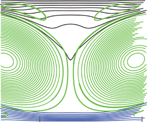
Figure 4. (a) Contours of total vorticity for a run with  $R{a^{\prime}_C} = 1.5 \times {10^6}$,
  ${S_0} = {10^3}$ and
  ${\gamma _n} = {10^3}$. (b) Flow in the indicated box has 50 streamfunction contours (green) and nine density contours (black). (c) Contours of
  ${\omega _b}$, the vorticity produced by buoyancy alone.

Figure 5. As in figure 4 but with  $R{a^{\prime}_C} = {10^6}$,
  ${S_0} = {10^3}$ and
  ${\gamma _n} = 0$. (a) Contours of total vorticity (every 2000). (b) Streamfunction (50 green contours) and density (black and blue contours every 0.1). (c) Contours of
  ${\omega _b}$, vorticity produced by buoyancy alone (every 2000).
The dynamics leading to double bulges is illustrated by figure 4 for runs at  $R{a^{\prime}_C} = 15 \times {10^5}$. Figure 4(a) shows contours of the total vorticity (the driving cell vorticity is added to the buoyancy-produced vorticity). There is comparable vorticity magnitude but opposite signs near the centre and along the flanks of the composition clusters. Figure 4(b) shows the streamfunction and composition fields. Out of 50 streamfunction contours, only two intersect the clusters. This shows that vertical speed within each cluster is very slow. The cluster contours show how the double bulges exist throughout the depth of the cluster. Figure 4(c) shows how buoyancy driven vorticity
  ${\omega _b}$ is concentrated near a production location at the double bulge flanks.
The double bulges and the circulation producing them are clearly linked to  ${\omega _b}$, the vorticity that is produced by buoyancy at the flanks of the clusters. When
  ${\omega _b}$ is approximately the same magnitude as the vorticity of the driving cells, the combined driving and buoyant cells produce tilted cells. This creates a wide region of very small vertical flow near each cluster. This small speed is illustrated by the fact that in figure 4(b), only two streamlines out of 50 intersect the cluster.
Figure 5 shows a steady flow with  ${\gamma _n} = 0$. The top and bottom layers are thicker possibly due partly to a smaller composition density difference
  $R{a^{\prime}_C} = {10^6}$ and the convection cells are markedly oval and tilted. Counter-circulations exist in the light layer that produce localized upwelling in the middle of the cluster, and the double bulges are large and occupy much of the cluster. The vorticities near the flanks of clusters in figures 4 and 5 are like those in figure 3 and in some figures of Whitehead (Reference Whitehead2023). This indicates that this simplified driving flow catches the basic dynamics of the more complex flow.
One way to clearly see if there are one or two bulges is to plot the value of concentration C along a horizontal line at fixed depth below the top surface as in figure 6. There, contours at 5/64 depth below the top are shown for seven values of  ${S_0}$ with
  $R{a^{\prime}_C}$ and
  ${\gamma _n}$ at fixed values. The transitions from a contour with one maximum for
  ${S_0} = 10$, 100 and 200 to contours with two maxima for the intermediate values
  ${S_0} = 500$, 1000 and 2000 and then back to one for
  ${S_0} = 3000$ are quite clear.

Figure 6. Profiles of concentration C across four cells as in figure 4 at a depth of 5/64 (0.078) below the top for seven different values of  ${S_0}$
  $(R{a^{\prime}_C} = 1.5 \times {10^6},{\gamma _n} = {10^3})$.
The presence of single or double bulges can be quantified using profiles like those in figure 6 with numerous plots varying either speed or  $R{a^{\prime}_C}$ while holding the other one fixed. The profiles can be used to generate a contour plot as in figure 7. In this case, for
  ${S_0} = {10^3}$ and
  ${\gamma _n} = {10^3}$, double maxima exist in the range
  $3.1 \times {10^5} < R{a^{\prime}_C} < 5 \times {10^6}$.

Figure 7. Contours of C with 0.1 intervals for one cell at a depth of 5/64 (0.078) as a function of  $R{a^{\prime}_C}$ for one pair of cells with fixed speed
  $({S_0} = {10^3},{\gamma _n} = {10^3})$. Double bulges replace single ones above the dashedblack line.
Next, covering a wide range of values of  $R{a^{\prime}_C}$ and
  ${S_0}$ for contours like figure 7, a regime diagram over
  $R{a^{\prime}_C}$ and
  ${S_0}$ parameter space with
  ${\gamma _n} = {10^3}$ can be constructed (figure 8). Double bulges occur above the black solid curve with the values for transition shown by stars. The break in the curve is not well resolved due to the limited number of stars. There is an upper limit for double bulges shown as the dashed black line with
  ${S_0} < 150$, but it is off the range of figure 7 for greater
  ${S_0}$. Specifically, curves like those in figure 6 have lateral variation (<1 %) for
  $R{a^{\prime}_C} > 4 \times {10^5},{S_0} < 200$ with
  ${\gamma _n} = {10^3}$, so the existence of extrema and their sizes are not well resolved and deemed negligible. Single maxima with flows like figure 3(a) occur below the solid black curve and for
  ${S_0} < 150$.

Figure 8. Transition values (black symbols and black curve by eye) and ranges in  $R{a^{\prime}_C}- {S_0}$ space for single and double bulges with
  ${\gamma _n} = {10^3}$. Also, values of maximum buoyancy-driven vorticity at transition (red line) and value of vorticity for the driving cells (red dashed line). Double bulges disappear above the blackdashed line.
The maximum value of vorticity for the buoyancy-driven flow and for the driving cells is also plotted. Although the buoyancy-driven vorticity is smaller than the vorticity of the driving cells, the vorticity near the double bulge would be great enough to have the total change sign.
5. Discussion
As  $R{a^{\prime}_C}$ increases, some trends are found in both configurations. Figure 2, from cellular convection (like Whitehead Reference Whitehead2023) and figures 3 and 7, from the simplified system, all show that as
  $R{a^{\prime}_C}$ increases: (1) a single bulge gives way to double bulges; (2) the double bulges spread apart; (3) amplitude of the double bulges decreases; (4) a wide flat region forms in between bulges. In addition, both figures 2 and 3 show that the speed of flow slows in the bulge region. These all are evidence that the simplified system contains all the dynamics needed for double bulges.
The fact that double bulges exist for layers limited by the two different processes of diffusion of the concentration alone (§ 3 and beyond) and double diffusion and restoration (in § 2 and Whitehead Reference Whitehead2023) is consistent with the idea that neither double diffusion nor restoration is needed for double bulges. The mechanism clearly originates from buoyant fluid stresses that produce vorticity. The buoyant component of the flow  ${\boldsymbol{u}}_b$ always produces vorticity opposite in sign to the driving cell vorticity. Double bulges exist when buoyant vorticity is large enough to make flows large enough to distort the driving cells.
Although this is simple and sensible, no reports of the double bulges for layers above infinite Prandtl number convection seem to exist in the literature. This seems odd, but since large ranges of parameter space do not satisfy this constraint, perhaps this explains why double bulges have not been found before. Of course, perhaps the present simulations do not apply for viscous cellular flow with two distinct immiscible layers rather than the diffusive layer used in this study. A definite proof for double bulges with immiscible layers is not present so far, but the present results indicate that the vorticity considerations would probably hold even for two distinct layers so that layered flows with distinct interfaces might have similar results. The contour shapes in figure 6 seem to be all similar within the range of double bulges. Possibly an exact solution for interface configuration exists, although none is presently known.
This study was motivated by a desire to quantify the effects of the buoyancy forces from lighter continental material in Earth's mantle convection. The presence of simple flows that produce double bulges and the understanding of the vorticity producing them might help to understand the general problem of the construction of continents through mountain building and orogeny (Whitehead Reference Whitehead2023). The differential stress along the base of continental crust that leads to convergence of crust and mountain building certainly acts like the vorticity that produces double bulges.
Double bulges that are generated by thickening at the flanks of clusters of lighter material at sinking regions were a surprise. Other aspects might exist in extensions to this study, so additional work would be useful. Hopefully, this simple study might stimulate new inquiries in this direction. For the Earth, the vorticity produced by the lower-density continent material, and its opposite sign to vorticity produced by subducting slabs, might be verified by seismic analysis. For fluid mechanics, extension to three dimensions (both Cartesian and spherical) and to flow with variations of properties would be interesting. Whether double bulges extend to flows with compositional or temperature-dependent viscosities could also be fruitfully explored.
Acknowledgements
No external support exists for this work.
Funding
This research received no specific grant from any funding agency, commercial or not-for-profit sector.
Declaration of interests
The author reports no conflict of interest.


 Open access