


1. Introduction
The dynamics of oscillating stratified boundary layers on sloping bathymetry may be an important mechanism of diapycnal water mass transformation in the context of the global overturning circulation of the ocean (Ferrari et al. Reference Ferrari, Mashayek, McDougall, Nikurashin and Campin2016). A fundamental understanding of the dynamical pathways between laminar, transitional and turbulent states is lacking. Historically, analyses of turbulent flows begin by answering the questions: how stable is the flow to linear disturbances, what are the relevant mechanisms of linear instability, and how does disturbance growth change as a function of the relevant non-dimensional parameters? We examine the linear stability of the laminar boundary layers that form as internal waves heave isopycnals up and down infinite slopes to answer these questions for oscillating stratified boundary layers on sloping bathymetry. Our use of a semi-infinite, constant-slope model is justified by the large separation of length scales between the viscous length scale of the laminar boundary layers,  ${O}(1)$ cm, and the internal-wave-generative abyssal slope length scales of
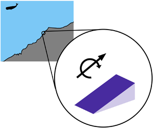
  ${O}(10)$ km (Jayne & St. Laurent Reference Jayne and St. Laurent2001; Goff & Arbic Reference Goff and Arbic2010). The geometry and scales that are typical of these boundary layers are illustrated by figure 1.

Figure 1. Illustration of Boussinesq boundary layers on abyssal slopes arising from the heaving of density surfaces up and down slope by internal waves with wavelengths  ${O}(10)$ km.
In the absence of shear, gravitational instabilities are often linear instabilities, as is the case for Rayleigh–Taylor and Rayleigh–Bénard instabilities. In sheared, gravitationally unstable flows, the transition pathways can be more complicated. Theoretical and experimental evidence suggest that two-dimensional rolls, initiated by linear near-wall gravitational instabilities and subsequently sheared into bursts of three-dimensional turbulence, are the dominant transition-to-turbulence mechanism in gravitationally unstable Couette flow (Bénard & Avsec Reference Bénard and Avsec1938; Chandra Reference Chandra1938; Brunt Reference Brunt1951; Deardorff Reference Deardorff1965; Gallagher & Mercer Reference Gallagher and Mercer1965; Ingersoll Reference Ingersoll1966). Similar mechanisms have been observed in direct numerical simulations (DNS) data of oscillating Boussinesq boundary layers on adiabatic sloping boundaries, which are a potentially important regime in the context of abyssal water mass transformation (Kaiser Reference Kaiser2020). In this paper, the linear stability of the non-rotating boundary layers is calculated to determine if the gravitational instability is a significant linear instability across a much broader region of parameter space than can be sampled by DNS.
The linear stability of stationary flows is conventionally analysed by introducing infinitesimal disturbances to the flow and linearizing the governing equations about the stationary base flow to form governing equations for the growth or decay of the infinitesimal disturbances (Lin Reference Lin1955; Drazin & Reid Reference Drazin and Reid1982; Schmid & Henningson Reference Schmid and Henningson2001). There are two standard techniques for linear stability analyses of time-periodic flows, instantaneous instability theory (IIT), also referred to as ‘quasi-static’ instability theory (Davis Reference Davis1976; Cowley Reference Cowley1987), and Floquet global instability theory (Von Kerczek & Davis Reference Von Kerczek and Davis1974; Hall Reference Hall1984; Blennerhassett & Bassom Reference Blennerhassett and Bassom2002). IIT refers broadly to the ad hoc application of the linear stability analysis of stationary flows to examine the stability of a time-dependent base flow at a chosen instant in time (Von Kerczek & Davis Reference Von Kerczek and Davis1976; Blondeaux & Vittori Reference Blondeaux and Vittori2021), although for some flows IIT can be justified formally through asymptotic expansion (Cowley Reference Cowley1987; Wu & Cowley Reference Wu and Cowley1995). One example is the case of Stokes’ second problem, also referred to as Stokes layers in the literature (Von Kerczek & Davis Reference Von Kerczek and Davis1974; Hall Reference Hall1984), where the Orr–Sommerfeld equation is solved for the growth rates of disturbances to base flow at a chosen instant in the period. To evaluate the global stability, or stability over the entire period, the instantaneous stability calculation must be performed over many instants within the period. If one or more instantaneous modes exhibit positive growth rates throughout the period, then the flow is globally unstable according to IIT (Luo & Wu Reference Luo and Wu2010). However, the validity of the IIT approach rests on the assumption that the instantaneous growth rates are much larger than the frequency of the base flow, i.e. the quasi-steady flow assumption. IIT has proved to be a successful and predictive approach for assessing the growth of Stokes layer shear instabilities at moderate to high Reynolds number (Luo & Wu Reference Luo and Wu2010), possibly because instantaneous mode growth rates increase as a function of Reynolds number (Monkewitz & Bunster Reference Monkewitz and Bunster1987). Hall (Reference Hall1984) used IIT to identify time-periodic Taylor–Görtler instabilities in centrifugal flows that are mathematically analogous to the time-periodic Rayleigh–Bénard-like instabilities investigated in this study.
Floquet instability theory (Floquet Reference Floquet1883) pertains to the net growth or suppression of instabilities over the course of one period. All periodic instantaneous globally unstable linear modes are unstable Floquet modes, but the opposite is not true: an unstable Floquet mode can correspond to linear energy exchange between two or more instantaneous modes that do not produce IIT global instability (Luo & Wu Reference Luo and Wu2010). Therefore, the evolution of a Floquet mode over a period does not necessarily correspond to the evolution of an instantaneous instability that occurs during that period, but it does represent the global effect of linear instantaneous instabilities. While Floquet instability theory is a mathematically rigorous approach to assessing the global linear stability of time-periodic flows, it does not extend to flows in which nonlinear instabilities are amplified on time scales shorter than the base flow period (Wu & Cowley Reference Wu and Cowley1995).
In this paper, we examine gravitational instabilities in laminar oscillating flow on adiabatic slopes in which the oscillatory forcing is oriented in the across-isobath direction for parameter regimes typical of super-inertial dynamics in abyssal ocean at low to middle latitudes. First, we define the Floquet stability problem, and second, we discuss our numerical methodology. Third, we discuss the neutral stability curves over a broad range of subcritical and supercritical slopes, before concluding.
2. Problem formulation
Even in the absence of an oscillatory body force, motion arises in Boussinesq diffusive boundary layers on adiabatic sloping boundaries because baroclinic vorticity is created by the tilting density surfaces parallel to the wall-normal axis, such that the angle  $\theta$ separates density surfaces from the hydrostatic pressure gradient in the vertical within the diffusive boundary layer (see figure 2). The production mechanism of baroclinic vorticity is oriented in the along-isobath, constant isobath direction (
 $y$ axis in figure 2), which drives across-isobath wall-parallel flows with a net upslope transport. Phillips (Reference Phillips1970) and Wunsch (Reference Wunsch1970) simultaneously derived analytical solutions for these laminar flows that were validated by the laboratory experiments of Peacock, Stocker & Aristoff (Reference Peacock, Stocker and Aristoff2004).

Figure 2. Coordinate system and vorticity components.
The addition of an oscillating body force in the across-isobath direction ( $x$ axis in figure 2) gives rise to a class of boundary layers that, in various limits, collapse to familiar classical oscillating boundary layers (e.g. Stokes’ second problem if the stratification vanishes, Stokes–Ekman layers in a rotating reference frame, Stokes buoyancy layers if
  $\theta ={\rm \pi} /2$, etc.), and it is representative of the frictional interaction of low-mode extra-critical baroclinic tidal flows in the ocean. The term ‘extra-critical’ refers to both subcritical and supercritical slopes at angles that are sufficiently smaller/larger, respectively, than the critical slope, where topographic–tidal resonance and other critical-slope effects are not dominant. Baidulov (Reference Baidulov2010) derived the linear solutions for the oscillating, stratified, viscous and diffusive boundary layer in a stationary (not rotating) reference frame (hereafter the oscillating boundary layer, OBL) and found that the linear flow is a superposition of two evanescent modes. Baidulov (Reference Baidulov2010) noted that the phase of one of the boundary layer modes changes sign as the slope increases from subcritical to supercritical, where critical slope is defined by the slope angle
  $\theta _c$ that satisfies
  $\omega =N\sin \theta _c$, and
  $N$ is the buoyancy frequency. The criticality parameter, defined by dimensional analysis of the governing equations, is
 \begin{equation} {C}=\frac{N\sin\theta}{\omega},\end{equation}
where if  $\theta =\theta _c$, then
  ${C}=1$, and subcritical and supercritical slopes can be defined as
  ${C}<1$ and
  ${C}>1$, respectively. The change in sign of the boundary layer solution mode indicates that the boundary layers share some of the dynamics of the parent flow (i.e. the larger-scale internal wave field in the oceanic example), which undergoes a change of sign of the group velocity of the radiated or reflected internal waves as the slope angle increases from subcritical to supercritical topography. At critical slope, the flow resonates because the across-isobath motions of the internal tide force the flow at the same frequency as that of the buoyant restoring force component in the across-isobath direction.
A commonly observed OBL flow feature is the formation and growth of gravitational instabilities produced by the upslope advection of relatively heavy water over relatively light water trapped at the boundary by friction. The energy source for the boundary layer gravitational instabilities investigated here is the baroclinic tide. Baroclinic tides are internal waves generated in response to oscillating stratified flow over variable bathymetry by the forcing of the barotropic tide. The interaction of the barotropic tide and the bathymetric variations can induce resonance near the boundary, such as overturning formed by critically reflecting internal waves (Dauxois & Young Reference Dauxois and Young1999) and the nonlinear baroclinic tide generation at critical slope (Gayen & Sarkar Reference Gayen and Sarkar2011; Rapaka, Gayen & Sarkar Reference Rapaka, Gayen and Sarkar2013; Sarkar & Scotti Reference Sarkar and Scotti2017). The barotropic tide can directly force stratified boundary layers over flat bathymetry: Von Kerczek & Davis (Reference Von Kerczek and Davis1976) and Gayen & Sarkar (Reference Gayen and Sarkar2010) investigated the dynamics of these flows by linear stability analysis and by large eddy simulation, respectively. However, gravitational instabilities at critical slope are formed by primarily inviscid nonlinearities in the baroclinic response to the barotropic tide (Dauxois & Young Reference Dauxois and Young1999), whereas the OBL gravitational instabilities are formed by viscous, insulating boundary conditions (Hart Reference Hart1971). OBL gravitational instabilities on extra-critical slopes have been observed in experiments (Hart Reference Hart1971), and observed in OBLs in lakes associated with internal seiche waves (Lorke, Peeters & Wüest Reference Lorke, Peeters and Wüest2005) and internal gravity waves (Lorke, Umlauf & Mohrholz Reference Lorke, Umlauf and Mohrholz2008). Similar boundary layer gravitational instabilities have been observed in the flood (i.e. upslope) phase of estuarine tidal flows (Simpson et al. Reference Simpson, Brown, Matthews and Allen1990; Chant & Stoner Reference Chant and Stoner2001; Geyer & MacCready Reference Geyer and MacCready2014), formed by a combination of bottom friction and the straining of horizontal buoyancy gradients over shallow finite topography.
Supercritical-slope OBL laboratory experiments by Hart (Reference Hart1971) identified spanwise plumes and rolls (described by the streamwise, or across-isobath vorticity component), associated with the periodic reversals of the density gradient, that resembled qualitatively the rolls that appeared in high-Rayleigh-number Couette flow experiments by Bénard & Avsec (Reference Bénard and Avsec1938), Chandra (Reference Chandra1938) and Brunt (Reference Brunt1951). Perhaps due to the similarity to the convection experiments, the rolls observed by Hart (Reference Hart1971) are often referred to as ‘convective rolls’ although the term is misleading because it implies diabatic boundary conditions; the gravitational instabilities, rolls and overturns of interest in this study are generated by adiabatic boundary conditions. Linear stability analyses by Deardorff (Reference Deardorff1965), Gallagher & Mercer (Reference Gallagher and Mercer1965) and Ingersoll (Reference Ingersoll1966) revealed that the observed growth of gravitationally unstable disturbances in high-Rayleigh-number Couette flows is suppressed in the plane of the shear (the streamwise vertical plane) by the shear itself (i.e. the suppression of the spanwise vorticity disturbances). However, they also found that the growth of disturbances in the spanwise-vertical plane (streamwise vorticity disturbances) is unimpeded by the shear and grows in the same manner as pure convection. It has since been established that streamwise (the across-isobath direction) vortices with axes in the direction of a mean shear flow (a.k.a. ‘rolls’) can arise due to heating or centrifugal effects (Hu & Kelly Reference Hu and Kelly1997). Therefore, since the upslope phase of the OBL is dynamically similar to gravitationally unstable Couette flow, we hypothesize that linear streamwise vorticity disturbances may be an important mode of instability in OBLs.
In this study, we analyse the Floquet stability of the coupled streamwise vorticity component ( $\zeta _1$, pointing in the across-isobath
  $x$ direction in figure 2) and buoyancy anomaly (aligned with the
  $\boldsymbol {\eta }$ coordinate in figure 2) in a diffusive, Boussinesq flow on an adiabatic slope when forced by an oscillating body force that represents the pressure gradient of a low-wavenumber internal wave,
 \begin{equation} F(t)={-}A \sin t, \end{equation}
where  $A$ is the amplitude of the non-dimensional pressure gradient, and
  $x$ is the across-isobath coordinate (up/down the slope). The coordinate system, rotated angle
  $\theta$ counterclockwise from horizontal, and the vorticity components are shown in figure 2.
2.1. Stationary and oscillating base flow components
The Boussinesq, dimensional forms of the conservation equations for mass and momentum are
 $$\begin{gather} \boldsymbol{\nabla}\boldsymbol{\cdot}\tilde{\boldsymbol{u}}=0, \end{gather}$$
 $$\begin{gather}\partial_t \tilde{\boldsymbol{u}} +\tilde{\boldsymbol{u}}\boldsymbol{\cdot}\boldsymbol{\nabla}\tilde{\boldsymbol{u}} ={-}\boldsymbol{\nabla} \tilde{p}+ \nu\,\nabla^2\tilde{\boldsymbol{u}} +(\tilde{b}\sin\theta+F(t))\,\boldsymbol{i}+\tilde{b}\cos\theta\, \boldsymbol{k}, \end{gather}$$
 $$\begin{gather}\partial_t\tilde{{b}}+\tilde{\boldsymbol{u}}\boldsymbol{\cdot}\boldsymbol{\nabla}\tilde{b} =\kappa\,\nabla^2\tilde{b}, \end{gather}$$
where  $\theta$ is the counterclockwise angle of the slope from horizontal, and the coordinates
  $\boldsymbol {i}$,
  $\boldsymbol {j}$ and
  $\boldsymbol {k}$ point in the across-isobath, along-isobath and wall-normal directions, respectively. Also,
  $\kappa$ is the molecular diffusivity of buoyancy, and
  $\nu$ is the molecular kinematic viscosity of abyssal seawater. The buoyancy is defined by density anomalies from the background flow,
  $\tilde {b}=g(\rho _0-\tilde {\rho })/\rho _0$, where
  $g$ is the gravitational acceleration,
  $\tilde {\rho }$ is the anomalous density, and
  $\rho _0$ is the reference density. The pressure
  $\tilde {p}$ is defined as the mechanical pressure divided by the reference density. The buoyancy frequency is defined by the hydrostatic background
  $N=\sqrt {-g/\rho _0((\partial \bar {\rho }/\partial x)\sin \theta +(\partial \bar {\rho }/\partial z)\cos \theta )}$ where
  $\bar {\rho }(x,z)+\rho _0$ is the hydrostatic background density field. The domain is semi-infinite, bounded only by a sloped wall at
  $z=0$ with no-slip, impermeable and adiabatic boundary conditions
 $$\begin{gather} \tilde{{\boldsymbol{u}}}(x,y,0,t)=0, \end{gather}$$
 $$\begin{gather}\partial_z\tilde{{b}}(x,y,0,t)=0. \end{gather}$$
At  $z\rightarrow \infty$, the flow has two components: a stationary, quiescent, stably stratified and hydrostatic component, and an across-isobath, adiabatic, balanced oscillation in the buoyancy, velocity and pressure fields. These two components prescribe the boundary conditions at
  $z\rightarrow \infty$:
 $$\begin{gather}
\tilde{{\boldsymbol{u}}}(x,y,\infty,t)={U}_{\infty}(t)\,{\boldsymbol{i}},
\end{gather}$$
$$\begin{gather}
\tilde{{\boldsymbol{u}}}(x,y,\infty,t)={U}_{\infty}(t)\,{\boldsymbol{i}},
\end{gather}$$
 $$\begin{gather}\partial_z\tilde{{b}}(x,y,\infty,t)=N^2\cos\theta. \end{gather}$$
Boundary conditions on the pressure field are satisfied automatically because the pressure field is diagnosed analytically from the other variables for both flow components. Let the prognostic variables be decomposed linearly into two components, denoted by the subscript ‘ $S$’ for the stationary component and the primed variables for the oscillating component:
 $$\begin{gather} \tilde{{\boldsymbol{u}}}(y,z,t)= {\boldsymbol{u}}_{{S}}(z)+{\boldsymbol{u}}'(y,z,t), \end{gather}$$
 $$\begin{gather}\tilde{b}(x,y,z,t)=b_{{S}}(x,z)+b'(y,z,t). \end{gather}$$
The stationary flow has no variability, other than hydrostatically balanced gradients, in the wall-tangent directions such that  $\partial _x=\partial _y=0$, and contains non-zero velocities only in the across-isobath component within a diffusion-driven boundary layer at the wall. The stationary flow is itself a linear superposition of a diffusion-driven boundary layer component and a quiescent, hydrostatic background component, and the stationary flow solutions were derived by Phillips (Reference Phillips1970) and Wunsch (Reference Wunsch1970).
Let us decompose the oscillating component into two components: a base flow component that is the hydrostatic response to the across-isobath momentum forcing, shown in (2.2), which includes a boundary layer in which friction and the diffusion of the adiabatic boundary condition break the inviscid balance of across-isobath heaving of isopycnals, and infinitesimal disturbances to the buoyancy and across-isobath vorticity:
 $$\begin{gather} {{\boldsymbol{u}}}'(y,z,t)= {\boldsymbol{U}}(z,t)+\epsilon\,\hat{{\boldsymbol{u}}}(y,z,t), \end{gather}$$
 $$\begin{gather}{b}'(y,z,t)=B(z,t)+\epsilon\,\hat{b}(y,z,t), \end{gather}$$
where  $0<\epsilon \ll 1$ and the capitalized variables represent the base flow, and the hatted variables represent the infinitesimal disturbances. The base flow solutions include only an across-isobath velocity component, and zero variability in the wall-tangent directions (
 $x$ and
  $y$) is also assumed for the base flow component.
The forcing amplitude of the oscillations,  $A$, is prescribed uniquely by the linear internal wave solution for a wave that is generated or reflected by a topographic feature, where the horizontal length scales of both the topographic feature and the internal wave are much greater than the relevant boundary layer length scales. The governing equations for the inviscid internal waves (characterized by horizontal length scales of
  ${O}(10)$ km) on the relatively small length scale
  $L={O}(10)$ m (see figure 1) can be approximated by reducing (2.3)–(2.5) to
 $$\begin{gather} \partial_t{{U}_{\infty}}= {B}_{\infty}\sin\theta-A\sin t, \end{gather}$$
 $$\begin{gather}\partial_t{{B}_{\infty}} ={-}{U}_{\infty}N^2\sin\theta, \end{gather}$$
where it is assumed that (a) there is no variability in any direction for the momentum and buoyancy, and (b) the flow is adiabatic and quiescent in the along-isobath and wall-normal directions everywhere ( $V_{\infty},W_{\infty}=0$) over length scale
  $L$. The solutions to the balanced, inviscid oscillations governed by (2.14) and (2.15) are
 $$\begin{gather} U_{\infty}(t)={-}U_0\cos t, \end{gather}$$
 $$\begin{gather}B_{\infty}(t)= B_0\sin t, \end{gather}$$
if and only if
 \begin{equation} A=U_0\omega({C}^2-1) \end{equation}
is satisfied, where  $\omega$ is the forcing frequency, and
  $U_0$ is the forcing velocity amplitude. The momentum and buoyancy amplitudes
  $U_0$ and
  $B_0$ must satisfy
 \begin{equation} \frac{B_0}{U_0}=CN. \end{equation}
Equation (2.18) diagnoses the internal wave forcing amplitude if  $\omega$,
  $C$, and
  $U_0$ are known, as is generally the case for abyssal slopes, and it indicates that the local approximation of an isopycnal heaving by a large horizontal wavelength internal wave on a similarly large horizontal wavelength topographic feature breaks down (
 $A\rightarrow 0$) as the slope angle vanishes ,
  $\theta \rightarrow 0$ , or slope-parallel buoyancy oscillations resonate with the forcing
  ${{C}\rightarrow 1}$, a.k.a. critical slope. This is consistent with internal wave theory, which indicates that no linear internal waves are generated by flat bathymetry, and that at critical slope, internal waves become highly nonlinear (Dauxois & Young Reference Dauxois and Young1999).
Baidulov (Reference Baidulov2010) derived solutions to the base flow,
 \begin{align} U({z},t)&=U_0\,{\rm Re}\left[ \left((\alpha_1+ \text{i}\alpha_2)\exp({(1+\text{i}){z}\phi_1/\delta_1})\right.\right.\nonumber\\ &\quad \left.\left.{}+ (\alpha_3+ \text{i}\alpha_4) \exp({(1+\text{i}){z}\phi_2/\delta_2}) -1 \right)\exp({\text{i}\omega{t}})\right], \end{align}
 \begin{align} B({z},t)&=B_0\,{\rm Re}\left[ \left((\beta_1+\text{i}\beta_2) \exp({(1+\text{i}){z}\phi_1/\delta_1})\right.\right.\nonumber\\ &\quad \left.\left.{}+(\beta_3+\text{i}\beta_4)\exp({(1+\text{i}){z}\phi_2/\delta_2})-1 \right)\text{i}\exp({\text{i}\omega{t}})\right], \end{align}
which satisfy the boundary conditions shown in (2.6), (2.7), (2.8) and  $\partial _zB(z\rightarrow \infty,t)=0$, thus satisfying (2.9). The real solutions for
  $U$ and
  $B$ are split into two sets of solutions corresponding to the sign of
 \begin{equation} \phi=\frac{\omega(1+\textit{Pr})}{\nu} -\sqrt{\frac{\omega^2(1+\textit{Pr})^2}{\nu^2}+4\,\frac{\textit{Pr}\,(N^2\sin^2\theta-\omega^2)}{{\nu^2}}}. \end{equation}
If the Prandtl number
 \begin{equation} \textit{Pr}=\frac{\nu}{\kappa} \end{equation}
is unity, then (2.22) simplifies to
 \begin{equation} \phi=\frac{2\omega}{\nu}\,(1-{C}), \end{equation}
thus whether the criticality parameter  ${C}$ is greater than or less than unity determines the base flow boundary layer dynamics. If
  ${C}=1$, then the base flow is an oscillation at the natural frequency of the system.
The fluid just above abyssal slopes is composed of Antarctic bottom water (AABW) over much of the low- to middle-latitude ocean, where AABW is characterized by temperatures approaching  $0\,^\circ {}{\rm C}$ from above and practical salinities approximately 35 psu. At
  $0\,^\circ {}{\rm C}$ and 35 psu, the kinematic viscosity is
  $1.83\times 10^{-6}\ {\rm m}^{2}\ {\rm s}^{-1}$, and the thermal diffusivity is
  $1.37\times 10^{-6}\ {\rm m}^{2}\ {\rm s}^{-1}$ (Chen et al. Reference Chen, Chan, Read and Bromley1973; Talley Reference Talley2011). Assuming that the density is a function of only temperature, the buoyancy diffusivity
  $\kappa$ might be interpreted as a coefficient of molecular thermal diffusivity. Therefore the molecular Prandtl number for seawater at AABW temperatures and pressures is
  $\textit {Pr}\approx 13$. However, we choose
  $\textit {Pr}=1$ to simplify base flow analytical solutions, where the solution coefficients for both subcritical and supercritical flows are provided in tables 1 and 2.
Table 1. Solution coefficients for subcritical slopes,  ${C}<1$. Here,
  $\delta _1$,
  $\delta _2$ and
  $L_b$ have units of length; all other variables are dimensionless.

Table 2. Solution coefficients for supercritical slopes,  ${C}>1$. Here,
  $\delta _1$,
  $\delta _2$ and
  $L_b$ have units of length; all other variables are dimensionless.

2.2. Ratio of stationary and oscillating flow component magnitudes
Across-isobath vorticity disturbances can be excited by the stationary flow component and/or the oscillating base flow component. The ratio of time scales and velocity magnitudes illustrates why, for the parameter ranges applicable to the abyssal ocean, the stationary flow can be neglected from Floquet analyses of the disturbances. The wall normal diffusive time scale is the relevant characteristic spin-up time scale of the stationary diffusion-driven flow because the diffusion of the adiabatic boundary condition into the interior induces the boundary layer baroclinic vorticity and momentum (Dell & Pratt Reference Dell and Pratt2015). Following Dell & Pratt (Reference Dell and Pratt2015), the spin-up time scale of the stationary flow component (Phillips Reference Phillips1970; Wunsch Reference Wunsch1970) is
 \begin{align} \tau_\kappa&\sim\delta_0^2/\kappa \end{align}
 \begin{align} &\sim\frac{\sqrt{\textit{Pr}}}{N\sin\theta}, \end{align}
where the boundary layer thickness of the stationary diffusion-driven boundary layer is
 \begin{equation} \delta_0=\left( \textit{Pr}\,\frac{N^2\sin^2\theta}{4\nu^2}\right)^{{-}1/4}. \end{equation}
Therefore, the modulation ratio (Davis Reference Davis1976) is
 \begin{equation} \mathcal{T}=\frac{\tau_\kappa}{\tau_\omega}\sim \frac{\omega\,\sqrt{\textit{Pr}}}{N\sin\theta}. \end{equation}
In the limit of  $\mathcal {T}\rightarrow \infty$, the time scale separation between the stationary diffusion-driven flow component and the oscillating flow component indicates that the slower stationary diffusion-driven flow component does not modulate the faster oscillatory flow component. If
  $\mathcal {T}\rightarrow 0$, then the oscillating flow component varies so slowly relative to the stationary diffusion-driven flow component that the steady flow component may alter the instabilities of the oscillating component.
The modulation ratios in (2.28) for typical abyssal parameter ranges for the  $M_2$ tide are shown in figure 3, which indicates that as
  $\theta \rightarrow 0$, the stationary diffusion-driven flow component does not modify the much faster dynamics of the oscillatory flow component. The time scale separation of at least
  ${O}(10^2)$, valid for approximately
  $0<\theta <1^\circ$ (0.0175 rad), a range of slopes commonly found in deep ocean bathymetry (Goff & Arbic Reference Goff and Arbic2010), informs our neglect of the stationary diffusion-driven flow component and application of Floquet analysis to the oscillatory flow component alone. While we consider the case
  ${\textit {Pr}}=1$, note that the time scale separation increases for
  ${\textit {Pr}}=10$.

Figure 3. The modulation ratio, the ratio of the spin-up time scale of the diffusion-driven component of flow to the tide period, for two different Prandtl numbers.
The characteristic velocity magnitude of the oscillating flow component is typically three orders of magnitude larger than the stationary flow component on abyssal slopes. The stationary diffusion-driven velocity magnitude is estimated by  $u_{S}\sim 2\kappa /\delta _0={O}(10^{-5}\unicode{x2013}10^{-6})\ {\rm m}\ {\rm s}^{-1}$ for
  $N=1.0\times 10^{-3}\ {\rm s}^{-1}$,
  $\nu =1.83\times 10^{-6}\ {\rm m}^{2}\ {\rm s}^{-1}$,
  $1\leqslant \textit {Pr}\leqslant 13$,
  $0<\theta \leqslant 10^\circ$. Characteristic baroclinic tide magnitudes
  $U\sim 0.01\ {\rm m}\ {\rm s}^{-1}$ are observed widely near abyssal slopes (Simmons, Hallberg & Arbic Reference Simmons, Hallberg and Arbic2004; Carter et al. Reference Carter, Merrifield, Becker, Katsumata, Gregg, Luther, Levine, Boyd and Firing2008; Goff & Arbic Reference Goff and Arbic2010; Turnewitsch et al. Reference Turnewitsch, Falahat, Nycander, Dale, Scott and Furnival2013) far from critical slopes, hydraulic spills and other turbulence ‘hot spots’.
2.3. Governing equations for along-isobath disturbances
The non-dimensional parameters of the linearized governing equations for the across-isobath vorticity component and buoyancy disturbances are chosen in the same manner as was used by Blennerhassett & Bassom (Reference Blennerhassett and Bassom2002) to investigate the linear stability of Stokes’ second problem, with the exceptions that we include the Boussinesq buoyancy and we analyse the across-isobath (streamwise) vorticity instead of the spanwise vorticity. The oscillating flow variables are non-dimensionalized as
 \begin{equation} {\boldsymbol{x}}=\frac{{\boldsymbol{x}}_{d}}{\delta}, \quad {{\boldsymbol{u}}}'=\frac{{{\boldsymbol{u}}}_{d}'}{U_0}, \quad t={\omega}{t_{d}}, \quad {p}'=\frac{{p}_{d}'}{U_0^2}, \quad {b}'=\frac{\omega{b}_{d}'}{N^2U_0\sin\theta}, \end{equation}
where subscript ‘ $d$’ denotes dimensional variables – and from here onwards, the variables without this subscript are dimensionless – and
  $\delta$ is the Stokes layer thickness, defined in (2.35). Also,
  ${p}'$ is the mechanical pressure divided by the reference density
  $\rho _0$, and the buoyancy is
  $b'=g(\rho _0-\rho ')/\rho _0$. Note that the Eulerian time scale is not proportional to the advective time scale (i.e.
  $U_0/\delta \neq \omega$). The two-dimensional flow governing equations for mass, momentum and thermodynamic energy (buoyancy) for the disturbances in the
  $y$–
$y$– $z$ plane are
 $$\begin{gather} 0=\partial_y\hat{v}+\partial_z\hat{w}, \end{gather}$$
 $$\begin{gather}\partial_t\hat{v}={-}\frac{\textit{Re}}{{2}}\,\partial_y\hat{p} +\frac{1}{2}\,(\partial_{yy}+\partial_{zz})\hat{v}, \end{gather}$$
 $$\begin{gather}\partial_t\hat{w}={-}\frac{\textit{Re}}{{2}}\,\partial_z\hat{p} +\frac{1}{2}\, (\partial_{yy}+\partial_{zz})\hat{w} +C^2\hat{b}\cot\theta, \end{gather}$$
 $$\begin{gather}\partial_t\hat{b}={-}\left(\frac{\textit{Re}\,\partial_zB(z,t)}{{2}}\right)\hat{w} +\frac{1}{2\,\textit{Pr}}\, (\partial_{yy}+\partial_{zz})\hat{b}, \end{gather}$$
where the Reynolds number and Stokes layer thickness are
 $$\begin{gather} \textit{Re}=\frac{U_0 \delta}{\nu}, \end{gather}$$
 $$\begin{gather}\delta=\sqrt{\frac{2\nu}{\omega}}. \end{gather}$$
For all analyses in this study,  $\textit {Pr}=1$. The streamwise vorticity component (see figure 2) is defined as
 \begin{equation} \hat{\zeta}_1=\partial_y\hat{w} -\partial_z\hat{v}. \end{equation}
Let the infinitesimal disturbances (hatted variables) take the form of a normal mode decomposition in the spanwise ( $y$) direction:
 $$\begin{gather} \hat{\zeta}_1(y,z,t)=\zeta_1(z,t)\,\mathrm{e}^{\text{i}ly} + \text{c.c.}, \end{gather}$$
 $$\begin{gather}\hat{b}(y,z,t)={b}(z,t)\,\mathrm{e}^{\text{i}ly} + \text{c.c.}, \end{gather}$$
where the modal streamfunction  ${\psi }$ and modal velocities are defined by
 $$\begin{gather} \zeta_1=(\partial_{zz}-l^2){\psi}, \end{gather}$$
 $$\begin{gather}(v,w)=(-\partial_z\psi,\text{i}l\psi), \end{gather}$$
 $$\begin{gather}l=l_{d}\delta{}=\frac{2{\rm \pi}}{\lambda}\,\delta, \end{gather}$$
where  $\lambda$ is the disturbance wavelength in the along-isobath direction. Finally, the governing equation for the evolution of the streamwise vorticity modes is
 \begin{equation} \partial_t\zeta_1= \underbrace{\frac{ \partial_{zz}-l^2}{2}\,{\zeta}_1}_{\text{diffusion}} \hspace{2mm}+\hspace{-3mm}\underbrace{\text{i}l{C}^2b\cot\theta }_{\substack{{\text{baroclinic}}\\ {\text{production of vorticity}}}}\hspace{-3mm}, \end{equation}
and the governing equation for the evolution of the associated buoyancy is
 \begin{equation} \partial_t{b}=\hspace{1mm} \underbrace{\frac{ \partial_{zz}-l^2}{2\,\textit{Pr}}\,b}_{\text{diffusion}}\hspace{1mm} -\hspace{1mm}\underbrace{\frac{\partial_zB(z,t)\,\text{i}l\,\textit{Re}}{{2}}\,{\psi}}_{\substack{{\text{advection of}}\\ {\text{base buoyancy}}}}. \end{equation}
There are no terms representing vorticity tilting or the advection of disturbances by the base flow in (2.42) and (2.43). The basic state flow enters the equations only through the advection of base flow buoyancy by the buoyancy disturbances (the first term on the right-hand side of (2.33)). Equations (2.42) and (2.43) indicate that the investigated instability is a manifestation of time-periodic Rayleigh–Bénard instability because the growth of disturbances is attributable solely to gravitational instabilities associated with the time-periodic boundary layer stratification. The state vector for (2.42) and (2.43) is
 \begin{equation} \boldsymbol{x}(z,t)= \begin{bmatrix} {\zeta}_1(z,t) \\ {b}(z,t) \end{bmatrix}, \end{equation}
and the dynamical operator for the evolution of the system is
 \begin{equation} \boldsymbol{A}(z,t)= \begin{bmatrix} \dfrac{\partial_{zz}-l^2}{2} & \text{i}lC^2\cot\theta \\[9pt] -\dfrac{\partial_zB(z,t)\,\text{i}l\,\textit{Re}(\partial_{zz}-l^2)^{{-}1}}{2} & \dfrac{\partial_{zz}-l^2}{2\,\textit{Pr}} \end{bmatrix}, \end{equation}
such that the evolution of the system is governed by
 \begin{equation} \frac{\mathrm{d}\kern0.7pt \boldsymbol{x}}{\mathrm{d}t}=\boldsymbol{A}\boldsymbol{x}, \end{equation}
where the operator  $\boldsymbol {A}(t)$ is periodic:
 \begin{equation} \boldsymbol{A}(z,t+T)=\boldsymbol{A}(z,t). \end{equation}
2.4. Boundary conditions
The oscillatory forcing was imposed by imposing a ‘moving wall’ boundary condition rather than applying a body force directly on the evolving modes. At the moving wall, the total flow boundary conditions on the momentum are no-slip and impermeable, therefore at  $z=0$,
 \begin{equation} \boldsymbol{u}' =U\boldsymbol{i}+\epsilon\hat{\boldsymbol{u}}=\cos{t}\,\boldsymbol{i}, \end{equation}
where  $0<\epsilon \ll 1$ is a small parameter, and
 \begin{equation} U(0,t)=\cos{t}, \end{equation}
therefore
 \begin{equation} \partial_{z}{\psi}=0 \end{equation}
is required to satisfy the no-slip condition at  $z=0$. The streamfunction must be constant along an impermeable wall, therefore it is numerically convenient to choose
 \begin{equation} \psi=0 \end{equation}
at  $z=0$ to satisfy
  $w=\partial _y\psi =0$. The wall is adiabatic, therefore
 \begin{equation} \partial_z{b}' =\partial_zB+\epsilon\,\partial_z\hat{b}=0. \end{equation}
Since the basic state stratification satisfies
 \begin{equation} \partial_zB=0, \end{equation}
the disturbance stratification must satisfy
 \begin{equation} \partial_z\hat{b}=0 \end{equation}
at  $z=0$.
At  $z\rightarrow \infty$, the boundary conditions for Stokes’ second problem are parallel and irrotational flow (Blennerhassett & Bassom Reference Blennerhassett and Bassom2002). Parallel flow is ensured if
 \begin{equation} \psi=0 \end{equation}
at  $z\rightarrow \infty$. Irrotational flow at
  $z\rightarrow \infty$ is prescribed by
 \begin{equation} \zeta_1=0. \end{equation}
The background hydrostatic stratification is constant in the far field, therefore at  $z\rightarrow \infty$, the base flow and disturbance stratification must be adiabatic:
 \begin{equation} \partial_zb=0. \end{equation}
2.5. Discrete Floquet exponents, modes and multipliers
Let the disturbance state vector  $\boldsymbol {x}$ be composed of two dynamical variables that vary in a single spatial dimension (
 $z$): the across-isobath vorticity
  $\zeta _1$ and the Boussinesq buoyancy
  $b$. Both variables are discretized onto a grid of
  $N_z$ discrete points in the
  $z$ coordinate:
 \begin{equation} \boldsymbol{x}(t)= \begin{bmatrix} \zeta_1(z_1,t) \\ \vdots \\ \zeta_1(z_{N_z},t) \\ b(z_1,t) \\ \vdots \\ b(z_{N_z},t) \end{bmatrix} = \begin{bmatrix} x_{1}(t) \\ \vdots \\ x_M(t) \end{bmatrix}, \end{equation}
where the length of state vector  $\boldsymbol {x}$ is
  $M=N_v\times N_z$ (the number of variables,
  $N_v$, multiplied by the number of grid points). The principal fundamental solution matrix
  $\boldsymbol {\varPhi }_p(t)$ for state vector
  $\boldsymbol {x}(t)$ is defined as
 \begin{equation} \boldsymbol{\varPhi}_p(t) = \begin{bmatrix} x_{1,1}(t) & \ldots & x_{1,M}(t)\\ \vdots & \ddots & \vdots \\ x_{M,1}(t) & \ldots & x_{M,M}(t) \end{bmatrix}, \end{equation}
such that each column of the principal fundamental solution matrix is the state vector for each separate initial condition for all  $N_z$ possible initial conditions. The principal fundamental solution matrix at time
  $t=T$ (where
  $T$ is the oscillation period) can be analysed to determine the fastest growing Floquet mode and discrete grid location of the largest Floquet multiplier (see Appendix A for the derivation and formal properties of the principal fundamental solution matrix). At time
  $t=0$, the principal fundamental solution matrix is an identity matrix that can be interpreted physically as a set of independent linear disturbances of the system; thus each Floquet mode represents an initial disturbance at each discrete grid location.
The innovation of Floquet (Reference Floquet1883) was the recognition that without loss of generality, the initial conditions specified at time  $t=t_0$ can be expressed in terms of the eigenvectors of the principal fundamental solution matrix after one oscillation period has elapsed,
  $t=t_0+T$. Floquet theory utilizes the principal fundamental solution matrix to calculate the mapping of the state vector from
  $t=t_0$ to
  $t=T$:
 \begin{equation} {\boldsymbol{x}}(T)=\boldsymbol{\varPhi}_p(T)\,{\boldsymbol{x}}(0), \end{equation}
where we have arbitrarily chosen  $t_0=0$. The eigenvectors of
  $\boldsymbol {\varPhi }_p(T)$ are mapped from
  $\boldsymbol {x}(0)$ to
  $\boldsymbol {x}(T)$ by the eigenvalues of
  $\boldsymbol {\varPhi }_p(T)$:
 \begin{equation} \boldsymbol{\varPhi}_p(T)\,\boldsymbol{x}_k(0)=\mu_k\,\boldsymbol{x}_k(0),\end{equation}
where  ${\mu }_k$ is the
  $k{\rm th}$ eigenvalue of
  $\boldsymbol {\varPhi }_p(T)$. The eigenvalues are the Floquet multipliers, and the real components of the multipliers indicate the stability of the system.
(i) If all Floquet multipliers satisfy
 ${\rm Re}[{\mu }_k]<1$, for $k=1,\ldots,M$ multipliers, then all disturbances decay as $t\rightarrow \infty$ and the system is stable.
(ii) If any Floquet multipliers satisfy
${\rm Re}[{\mu }_k]=1$, and the rest satisfy ${\rm Re}[{\mu }]<1$, then the stability of the system is periodic as $t\rightarrow \infty$.(iii) If any Floquet multiplier satisfies
${\rm Re}[{\mu }_k]>1$, then the disturbance will grow in amplitude as $t\rightarrow \infty$ and the system is unstable.


The Floquet exponents  $\gamma _k$ satisfy
 \begin{equation} \gamma_k = \frac{\log\mu_k}{T} \end{equation}
for each  $k{{\rm th}}$ eigenvalue, and the Floquet modes are defined as the solution of (2.46), with the initial conditions defined as the eigenvectors of (2.61), such that the modes satisfy
 \begin{align} {\boldsymbol{x}}_k(T)&=\mu_k\,{\boldsymbol{x}}_k(0) \end{align}
 \begin{align} &=\exp(\gamma_k T)\,{\boldsymbol{x}}_k(0). \end{align}
Additional Floquet theory details are provided in Appendix A.
3. Numerical methods
As described in § 2.5, the length of the disturbance state vector  $\boldsymbol {x}$ is
  $N_v\times {}N_z$, where
  $N_v$ is the number of variables, and
  $N_z$ is the number of grid points. In the streamfunction-vorticity formulation in this study,
  $N_v=2$ for vorticity and buoyancy. The number of grid points in
  $z$, the wall-normal direction, for all calculations was
  $N_z=200$. Therefore, the discrete principal fundamental solution matrix is a square matrix with
  $2N_z$ rows and columns. The variables were computed at the cell centres of a uniform grid of height
  $H/\delta =32$, where the non-dimensional grid encompassed
  $z=[0,H/\delta ]$. Previous studies found that Floquet stability calculations for Stokes’ second problem were unaffected by an upper domain boundary as long as it was located at
  $H/\delta =32$ or greater (Blennerhassett & Bassom Reference Blennerhassett and Bassom2006; Luo & Wu Reference Luo and Wu2010).
Centred second-order finite difference schemes were used to compute the discrete forms of all first and second derivatives, and the vorticity inversions that appear the dynamical operator  $\boldsymbol {A}(z,t)$. To implement the no-slip, impermeable boundary conditions at the wall, (2.50) and (2.51), the streamfunction and its
  $z$ derivative were set to zero. However, to guarantee unique solutions at second-order accuracy, the vorticity at the wall was required to compute the second derivatives of the vorticity. The second-order accuracy was confirmed with grid convergence tests shown in Appendix B. A second-order accurate extrapolation of the vorticity at the wall that accounts for no-slip and impermeable boundary conditions was derived by Woods (Reference Woods1954) for this purpose. The Woods (Reference Woods1954) boundary condition is
 \begin{equation} \zeta(0,t)=\frac{3}{(\Delta z)^2}\,\psi(z_1,t)-\frac{1}{2}\,\zeta(z_1,t), \end{equation}
where  $z=0$ denotes variables located at the wall, and
  $z=z_1$ denotes variables located at the first cell centre. All of the other boundary conditions (2.54), (2.55), (2.56) and (2.57) were implemented readily into the discrete derivatives within the discrete form of the operator
  $\boldsymbol {A}(z,t)$. Finally, test functions were used to ensure that the truncation error for all discrete derivatives and inversions decreased with
  $(\Delta z)^{-2}$, where
  $\Delta z$ is the height of a grid cell.
To obtain the principal fundamental solution matrix at time  $t=T$, (A5) was integrated over one period with the standard explicit fourth-order Runge–Kutta time advancement method, equivalent to solving simultaneously the evolution of the state vector in (2.46) in which each linearly independent solution begins with each linearly independent initial condition as defined in (A4). The method for computing the principal fundamental solution matrix in this study is formally second-order accurate.
3.1. Solver verification
The neutral stability curve for Stokes’ second problem was computed as a code verification test, shown in figure 4. There, the blue line is the computed neutral stability curve, and the pink line is a least squares fit of the computed neutral stability curve. The yellow line is a least squares fit of the computed stability curve by Blennerhassett & Bassom (Reference Blennerhassett and Bassom2002), who used a spectral method for the computation, and the blue dots were calculated by linearized direct numerical simulations by Luo & Wu (Reference Luo and Wu2010). The variations in the neutral stability curve about the pink line can be attributed to the spatial discretization method. This hypothesis is supported by the Floquet results for the neutral stability curve for Mathieu's equation (see Appendix B), which has no spatial derivatives and was computed to graphical accuracy using the same code for time integration and eigenvalue calculation.

Figure 4. The neutral stability curve for Stokes’ second problem. Verification of spatial discretization, temporal discretization and eigenvalue calculation. The computed Floquet multipliers are shown by the grey shading, and the calculated  ${\rm Re}[\mu ]=1$ contour is represented with the blue line. Here,
  $k$ is the streamwise wavenumber (analogous to the across-isobath wavenumber on a slope); see Appendix D for the governing equation for spanwise vorticity disturbances for Stokes’ second problem.
The irregularities of the blue neutral stability curve in figure 4 occur because of the combined effect of the initialization of the principal fundamental solution matrix as an identity matrix and finite difference spatial discretization. In the first time step of the calculation, the finite difference of discontinuous functions (specifically Dirac delta functions, one for each column of the principal fundamental solution matrix) introduces discretization errors (e.g. numerical dispersion from forward differences) that do not converge with increased grid resolution because the initial conditions remain an identity matrix for any possible grid resolution. Recall that Floquet theory requires that the principal fundamental solution matrix at time  $t=t_0$ must be an identity matrix. To verify that the discontinuities of the initial conditions are the source of non-convergent numerical error, the stability of Stokes’ second problem was computed for varied Reynolds numbers and grid resolutions at
  $k=0.35$, as shown in figure 5. The Floquet multipliers in figure 5 that correspond to stable points in the neutral stability plot of figure 4 converge quickly with increasing grid resolution. However, for
  $\textit {Re}\geqslant 1400$,
  $k=0.35$ (inside or near the unstable region of figure 4), the multipliers in figure 5 do not converge with increasing grid resolution. For comparison, the grid convergence of the derivative and inversion discretization was verified by using a smooth test function (Appendix C). Since the non-convergent error does not arise from the calculation of temporal or spatial derivatives of smooth functions, by process of elimination the non-convergent error must arise from the calculation of the spatial derivatives of the discontinuous functions at time
  $t=t_0$. Therefore, the neutral stability curves calculated by our finite difference method must be considered an approximate and conservative estimate.

Figure 5. Grid convergence occurs only for stable calculations. Stable Floquet multiplier calculations achieve grid convergence. Near the neutral stability curve, the Floquet multiplier calculations fail to achieve grid convergence because finite differences of the identity matrix initial condition of the principal fundamental solution matrix introduce grid independent noise. Therefore the ‘wiggles’ of the blue curve in figure 4 are due to the sensitivity of the multiplier value to noise introduced at just after  $t=0$ when finite differences are taken of discontinuities in the principal fundamental solution matrix.
4. Results
Figure 6 depicts the results of Floquet analysis of vorticity and buoyancy disturbances governed by (2.42) and (2.43), respectively, which indicate that the system is increasingly linearly unstable as the Reynolds number, criticality parameter and non-dimensional spanwise disturbance wavenumber are increased. Here,  $\textit {Re}<10$ and
  $l<0.5$, approximately, give maximum Reynolds number and disturbance wavelength required for stability for the entire investigated parameter space. At
  ${C}\ll 1$, the minimum Reynolds number necessary for global linear instability increases, and the forcing of vorticity disturbances by buoyancy disturbances decreases because the baroclinic production term on the right-hand side of (2.42) vanishes in the limit
  ${C}\rightarrow 0$. Therefore, increased stability at small
  ${C}\ll 1$ suggests that baroclinic production of disturbance vorticity is the primary mechanism of instability. This result is in agreement with the empirical and approximate stability criteria of Hart (Reference Hart1971), which posits that the flow is globally stable if
  ${C}^2\ll 1$.

Figure 6.  $\log _{10}({\rm Re}[\mu ])$ for the streamwise vorticity
  $\zeta _1$ for subcritical and supercritical slopes as functions of criticality parameter (
 ${C}=N\sin \theta /\omega$), Reynolds number (
 $\textit {Re}=U_0\delta /\nu$) and spanwise disturbance wavenumber (
 $l=2{\rm \pi} \delta /\lambda$). The pink lines are the Floquet neutral stability curves (
 ${\rm Re}[|\mu |]=1$,
  ${\rm Re}[|\gamma |]=0$).
If  $\omega$,
  $N$ and
  $\theta$ are constant, then (2.19) indicates that increasing the oscillation velocity amplitude
  $U_0$ and thus the Reynolds number will increase the amplitude of the buoyancy oscillations
  $B_0$ as well. Since the boundary layer thicknesses
  $\delta _1,\delta _2$ do not depend on
  $U_0$, and they determine the length scale of the boundary layer buoyancy gradient, the boundary layer buoyancy gradient increases with increasing Reynolds number, and both quantities force buoyancy disturbances through the second term on the right-hand side of (2.43).
The system is stable to small along-isobath wavenumber disturbances because all of the terms on the right-hand sides of (2.42) and (2.43) vanish except for the diffusion of disturbances in the wall-normal direction in the limit as  $l\rightarrow 0$. Growing disturbances described by (2.45) are confined to the boundary layer because they are forced by the base flow buoyancy gradient that vanishes outside the boundary layer; disturbances that propagate outside of the boundary layer are diffused.
The fingers on the neutral stability curves shown in figure 6 merit further examination by different numerical methods, particularly at  ${C}=1/2$,
  $3/4$ and
  $5/4$. The convergence of the time integration and spatial derivative schemes were verified independently (Appendices B and C), therefore by elimination, the irregularities in the neutral stability curves in figures 4 and 6 are attributed to the spatial discontinuities in the initial conditions of the principal fundamental solution matrix (A4). Nevertheless, comparison of the approximate behaviour of neutral stability curves in figures 4 and 6 suggests that the global gravitational instability is generally unstable at lower Reynolds numbers than Stokes’ layer instabilities.
Each equation term in matrix  $\boldsymbol {A}(z,t)$ (see (2.45)) was integrated in
  $z$ and
  $t$ for the fastest growing Floquet mode (the mode with maximum
  $\mu$, where
  $\mu >1$) to assess qualitatively the dominant physical mechanisms of the fastest growing linear disturbances. The terms were normalized by the total right-hand-side forcing, corresponding to the rows of
  $\boldsymbol {A}(z,t)$, such that the temporally and spatially integrated forcings sum to unity. The magnitudes of the equation terms, shown in figure 7, suggest that on both subcritical and supercritical slopes, the fastest growing linearly unstable disturbances are amplified by the non-diffusive terms in (2.42) and (2.43), and that the diffusive terms increasingly inhibit the growth of linear instabilities as
  ${C}\rightarrow 0$.

Figure 7. Integrated  $\zeta _1$,
  $b$ budgets for
  $\textit {Re}=420$,
  $l=1.0$. Percentages of the right-hand sides of (2.42) and (2.43) are calculated by spatio-temporal integration of
  $\boldsymbol {A}(z,t)$, for the most unstable Floquet mode at each value of
  ${C}$. The flow is Floquet unstable at
  $\textit {Re}=420$,
  $l=1.0$ for all
  $C$ investigated, therefore the dominant mechanisms induce disturbance growth.
The inherent three-dimensionality of the gravitational instability initiated by along-isobath buoyancy disturbances (2.38) to the across-isobath vorticity component is evident in the baroclinic vorticity production term of the governing equation for the total vorticity. The total baroclinic vorticity production can be derived by taking the curl of (2.4):
 \begin{equation} \substack{{\text{time rate of change of total}}\\ {\text{baroclinic vorticity production}}} =C^2(\text{i}l\,b(z,t)\,\mathrm{e}^{\text{i}ly}\cot\theta\,\boldsymbol{i} -\partial_zB\,\boldsymbol{j} -\text{i}l\,b(z,t)\,\mathrm{e}^{\text{i}ly}\,\boldsymbol{k}), \end{equation}
where the total vorticity is defined as  $\boldsymbol {\nabla }\times \tilde {\boldsymbol {u}}$. Equation (4.1) reveals that growing along-isobath buoyancy disturbances force the across-isobath and wall-normal vorticity components. This suggests that the growth of linear gravitational instabilities induced by along-isobath disturbances may induce three-dimensional motion, a phenomenon that is observed widely in stratified shear flow instabilities (Peltier & Caulfield Reference Peltier and Caulfield2003), and it suggests that the full three-dimensional dynamics may need to be considered to assess accurately the growth of linear modes as
  $t\rightarrow \infty$ because three-dimensional diffusive damping or other relaminarization mechanisms may affect the growth of unstable modes over the course of one period (Blondeaux, Pralits & Vittori Reference Blondeaux, Pralits and Vittori2021). DNS by Kaiser (Reference Kaiser2020) suggest that at low Reynolds number, the growth of linear instabilities is dissipated by three-dimensional chaotic motion. The total baroclinic vorticity production may also be necessary to describe the evolution of two-dimensional rolls in the along-isobath plane, initiated by gravitational instabilities, into three-dimensional motions and subsequently a relaminarized state as observed by Hart (Reference Hart1971) in experiments. Further experiments and DNS of relevant flows are needed.
5. Conclusions
Floquet linear stability theory was applied to laminar, oscillating, stratified, viscous diffusive boundary layers on infinite slopes in non-rotating reference frames. The linear stability of two-dimensional disturbances in the  $y$–
$y$– $z$ plane (described by the across-isobath vorticity
  $\zeta _1$) was evaluated within the non-dimensional parameter ranges
  $0<\textit {Re}\leqslant 1750$,
  $1/8\leqslant {C}\leqslant 7/4$,
  $0< l\leqslant 3$ and
  $\textit {Pr}=1$. The parameter regime is consistent with idealized
  $M_2$ tidal heaving of isopycnals up and down smooth, middle-latitude abyssal slopes where
  $N/\omega \sim 7.1$,
  $0<\theta \leqslant {\rm \pi}/12$,
  $\nu \sim 2.0\times 10^{-6} \ {\rm m}^2\ {\rm s}^{-1}$,
  $\omega \sim 1.4\times 10^{-4}\ {\rm rad}\ {\rm s}^{-1}$,
  $35.4\leqslant \lambda <\infty$ cm and
  $0.0< U_\infty \leqslant 2.1\ {\rm cm} \ {\rm s}^{-1}$. The most salient results of the Floquet analyses are as follows.
(i) Only the low along-isobath wavenumber modes,
$l\leqslant 0.1$, were stable for all $\textit {Re}$ investigated, corresponding to boundary layer disturbance wavelengths of approximately $\lambda \geqslant 0.3$ m on low- to midddle-latitude abyssal slopes.(ii) The critical Reynolds number (the lowest unstable Reynolds number for all along-isobath disturbance wavenumbers) decreases with increasing slope criticality, ranging from
$\textit {Re}\approx 300$ (corresponding to an oscillating abyssal tide amplitude $U_0\sim 10^{-3}\ {\rm m}\ {\rm s}^{-1}$) at $C=1/8$ to $\textit {Re}\approx 10$ (corresponding to an oscillating abyssal tide amplitude $U_0\sim 10^{-4}\ {\rm m}\ {\rm s}^{-1}$) at $C=3/4$ and $C=5/4$. Therefore our analysis predicts that oscillations of the $M_2$ tide at typical abyssal magnitudes ($U_0\sim 10^{-2}\ {\rm m}\ {\rm s}^{-1}$) are Floquet unstable to along-isobath gravitational disturbances characterized by wavenumbers $l\geqslant 0.1$, corresponding to wavelengths of approximately $\lambda \leqslant 0.3$ m.(iii) The mathematical description of the investigated linear instability is similar to that of the linear gravitationally unstable Couette flow (Ingersoll Reference Ingersoll1966), where the growth of along-isobath/spanwise buoyancy disturbances are not suppressed or excited by across-isobath/streamwise shear. The investigated instabilities may alternatively be considered as manifestations of time-dependent Rayleigh–Bénard instability. However, further experiments on the investigated flow in the range of parameter space relevant to abyssal slopes are needed, as are nonlinear and/or three-dimensional stability analyses.
(iv) Our finite difference numerical approach is more sensitive to numerical noise near the neutral stability curve than spectral methods. Temporal derivative discretization was verified by comparison with analytical Floquet solutions, and spatial derivative discretization was verified by grid convergence of the spatial derivatives and inversions for a smooth test function. Therefore, the source of the numerical errors near the neutral stability curves is attributable solely to finite difference errors arising from the approximation of the derivatives of the discontinuities in the identity matrix initial conditions. The identity matrix initial conditions are prescribed by Floquet theory and must remain an identity matrix regardless of grid resolution, thus the numerical errors of concern cannot be eliminated by increasing the grid resolution. Therefore, our finite difference method yields an approximate estimate of the extent of the neutral stability curve.


Acknowledgements
The authors thank the Massachusetts Green Computing Center, J. Callies, J. Canfield, R. Ferrari, K. Helfrich and A. Thurnherr. This document is approved for Los Alamos Unlimited Release, LA-UR-21-28221.
Funding
This work was supported by an NSF Graduate Research Fellowship for B.E.K., the Massachusetts Institute of Technology–Woods Hole Oceanographic Institution Joint Program, and the National Science Foundation (OCE-1657870).
Declarations of interests
The authors report no conflict of interest.
Appendix A. Floquet theory fundamentals
In this appendix, Floquet theory for tensors is summarized briefly to show how Floquet multipliers can be calculated directly for base flow solutions across spatial grids. The reader is referred to Iooss & Joseph (Reference Iooss and Joseph2012) for the complete derivation. In Floquet theory, the principal fundamental solution matrix is a mapping of the state vector  $\boldsymbol {x}$ at time
  $t=0$ to one period,
  $t=T$. For a state vector
  $\boldsymbol {x}(t)$ of shape
  $[M\times 1]$, where
  $M$ is the number of variables times the number of grid points, there exists a fundamental solution matrix
  $\boldsymbol {\varPhi }(t)$ of shape
  $[M\times {}M]$ and coefficient vector
  $\boldsymbol {c}$ of shape
  $[M\times 1]$ such that
 \begin{equation} {\boldsymbol{x}}(t)=\boldsymbol{\varPhi}(t)\,{\boldsymbol{c}} . \end{equation}
The fundamental solution matrix is a non-unique matrix in which the columns are the structure of the linearly independent solutions. The magnitudes of the elements in  $\boldsymbol {\varPhi }$ depend on the choice of
  $\boldsymbol {c}$, and the only restriction to the choice of a tenable
  $\boldsymbol {c}$ is that
  $\boldsymbol {\varPhi }$ be invertible. In that case, at time
  $t=0$,
 \begin{equation} \boldsymbol{c}=\boldsymbol{\varPhi}(0)^{{-}1}\,\boldsymbol{x}(0). \end{equation}
Substitution of (A2) into (A1) yields
 \begin{equation} {\boldsymbol{x}}(t)=\boldsymbol{\varPhi}(t)\,\boldsymbol{\varPhi}(0)^{{-}1}\,{\boldsymbol{x}}(0). \end{equation}
The principal fundamental solution matrix  $\boldsymbol {\varPhi }_p$ is just a fundamental solution matrix chosen such that at
  $t=0$, it is an identity matrix:
 \begin{equation} \boldsymbol{\varPhi}_p(0)=\boldsymbol{I}. \end{equation}
Substitution of (A4) into (A3) yields (2.60), therefore the principal fundamental solution matrix at time  $t=T$ maps the initial state
  $\boldsymbol {x}(0)$ to the final state after one period,
  $\boldsymbol {x}(T)$. By definition, (2.46) can be written in terms of the principal fundamental solution matrix,
 \begin{equation} \frac{\mathrm{d}\boldsymbol{\varPhi}_p}{\mathrm{d}t}=\boldsymbol{A}(t)\,\boldsymbol{\varPhi}_p(t), \end{equation}
so  $\boldsymbol {\varPhi }_p(T)$ can be obtained directly by integrating (A5) forward in time one period. The direct application of Floquet theory to a state vector describing a fluid flow has been used by Noack & Eckelmann (Reference Noack and Eckelmann1994), Robichaux, Balachandar & Vanka (Reference Robichaux, Balachandar and Vanka1999) and Barkley & Henderson (Reference Barkley and Henderson1996) to study instabilities in the periodic von Kármán vortex streets that develop in the wakes of cylinders.
Appendix B. Floquet analysis of Mathieu's equation
The Mathieu equation is an ordinary differential equation of the form
 \begin{equation} \partial_{tt}y+f(t)\,y=0, \end{equation}
where
 \begin{equation} f(t)=\delta+\varepsilon\cos(t). \end{equation}
The neutral stability curve of Mathieu's equation was computed to verify the temporal discretization and is shown in figure 8.

Figure 8. The neutral stability curve for Mathieu's equation; verification of the temporal discretization scheme and the eigenvalue calculation. The computed Floquet multipliers are shown by the grey shading, and the  ${\rm Re}[\mu ]=1$ contour lies under the yellow line of Kovacic, Rand & Sah (Reference Kovacic, Rand and Sah2018) to graphical accuracy.
Appendix C. Finite difference grid convergence
Second-order accurate finite difference stencils were used to form discrete matrices for the calculation of the first and second derivatives of the buoyancy disturbances (2.43), for the calculation of the second derivatives of the vorticity disturbances (2.42), and for calculating the streamfunctions by inverting the vorticity (2.39). Figure 9 shows the grid convergence of the buoyancy derivative stencils when applied to the test function  $b=\cos (2{\rm \pi} {}z/H)$. The test function for checking the inversions and vorticity derivatives,
 \begin{equation} \psi(z)=((z+1)^3-z^2-3z-1)\mathrm{e}^{{-}mHz}, \end{equation}
was chosen because it satisfies the same boundary conditions as were required for the Floquet analysis. The test  $\psi (z)$ is shown in figure 10. The grid convergence of the Woods (Reference Woods1954) vorticity boundary condition (which imposes no-slip and impermeable boundary conditions on the diffusion of vorticity), the second derivative of vorticity, and the inversion of vorticity to obtain the streamfunction are shown in figure 11.

Figure 9. Grid convergence of buoyancy derivatives.

Figure 10. Test function for  $\psi$.

Figure 11. Grid convergence of finite differences for the vorticity.
Appendix D. Stokes’ second problem governing equations
The governing equation for the spanwise vorticity disturbances is
 \begin{equation} \partial_t\zeta_2 =\underbrace{\frac{ \partial_{zz}-k^2}{2}\,{{\zeta}_2}}_{\text{diffusion}} -\underbrace{\frac{U{\rm i}k\,\textit{Re}}{2}\,{{\zeta}_2}}_{\substack{{\text{mean}}\\ {\text{advection}}}} +\underbrace{\frac{(\partial_{zz}U){\rm i}k\,\textit{Re}}{{2}}\,{\psi}}_{\substack{{\text{vorticity line tilting}}\\ {\text{by mean flow}}}} +\underbrace{{C}^2(\partial_{z} -{\rm i}k\cot\theta){b}}_{\substack{{\text{baroclinic}}\\ {\text{production of vorticity}}}}, \end{equation}
and the governing equation for the buoyancy disturbances in the  $x$–
$x$– $z$ plane is
 \begin{equation} \partial_t{b}= \underbrace{\frac{ \partial_{zz}-k^2}{2\,\textit{Pr}}\,b}_{\text{diffusion}} -\underbrace{\frac{U{\rm i}k\,\textit{Re}}{2}\,b}_{\substack{{\text{mean}}\\ {\text{advection}}}} +\underbrace{\frac{(\partial_zB){\rm i}k\,\textit{Re}}{{2}}\,{\psi}}_{\substack{{\text{advection of}}\\ {\text{mean buoyancy}}}}. \end{equation}
Equation (D2) and the baroclinic vorticity term in (D1) are eliminated for Stokes’ second problem, where  ${C}=0$ and
  $b(z,t)=0$. The remaining spanwise vorticity disturbance equation (Blennerhassett & Bassom Reference Blennerhassett and Bassom2006) was used to calculate the linear stability of Stokes’ second problem shown in figure 4:
 \begin{equation} \partial_t\zeta_2 =\frac{\partial_{zz}-k^2}{2}\,\zeta_2 -\frac{U{\rm i}k\,\textit{Re}}{2}\,\zeta_2 + \frac{(\partial_{zz}U){\rm i}k\,\textit{Re}}{{2}}\,\psi. \end{equation}


 Open access