Computational Study of a Vertical Plunging Jet into Still Water


1
Engineering College, Ocean University of China, Qingdao 266100, China
2
School of Environment Science and Spatial Informatics, China University of Mining and Technology, Xuzhou 221116, China
*
Author to whom correspondence should be addressed.
Water 2018, 10(8), 989; https://doi.org/10.3390/w10080989
Submission received: 29 May 2018
/
Revised: 12 July 2018
/
Accepted: 16 July 2018
/
Published: 26 July 2018
(This article belongs to the Section Hydraulics and Hydrodynamics)
Abstract
:The behavior of a vertical plunging jet was numerically investigated using the coupled Level Set and Volume of Fluid method. The computational results were in good agreement with the experimental results reported in the related literature. Vertical plunging jet characteristics, including the liquid velocity field, air void fraction, and turbulence kinetic energy, were explored by varying the distance between the nozzle exit and the still water level. It was found that the velocity at the nozzle exit plays an unimportant role in the shape and size of ascending bubbles. A modified prediction equation between the centerline velocity ratio and the axial distance ratio was developed using the data of the coupled Level Set and Volume of Fluid method, and it showed a better predicting ability than the Level Set and Mixture methods. The characteristics of turbulence kinetic energy, including its maximum value location and its radial and vertical distribution, were also compared with that of submerged jets.
1. Introduction
The plunging jet is of great importance in many practical applications, such as mineral-processing flotation cells, aeration and re-oxygenation of lakes and rivers, wastewater treatment, as well as oxygenation of mammalian-cell bioreactors [1,2,3]. When a water jet plunges into a liquid surface after passing through the surrounding air, it usually entrains a large amount of air into the receiving pool, and a complex mass transfer and energy exchange occurs between the water and air bubbles [4].
Many researchers have conducted experimental investigations on the plunging jet’s characteristics. Qu et al. [5] characterized a liquid plunging jet in a pool and the entrainment process using a variety of non-invasive flow visualization techniques and image analysis. McKeogh and Ervine [6] measured the velocity profile and the air distribution of a fully developed two-phase flow, and an empirical expression of centerline velocity was developed for the submerged jet region. Chanson [3] and Chanson et al. [7] determined an empirical relationship to predict the entrained air distribution and the plunging jet flow motion. Iguchi et al. [8] measured the mean velocity in both the radial and axial directions in the bubble dispersion region produced by a vertical water plunging jet in a transparent water bath. As a widely used parameter, the bubbly penetration depth for a plunging jet was also studied experimentally by Harby et al. [4], McKeogh and Ervine [6], Smigelschi and Suciu [9], and Cumming [10].
Numerical investigations are also used to characterize plunging liquid jets. For example, the Volume of Fluid (VOF) method was successfully used to capture the free-surface shape [11]. It was also employed to examine the air entrainment characteristics of a water jet plunging into a quiescent water pool for horizontal angles ranging from 10° to 90° [12]. Large Eddy Simulations and Volume of Fluid (LES-VOF) methods were employed for weakly and highly disturbed liquid plunging jets [13]. A modified hybrid multiphase flow solver has been used to simulate a vertical plunging liquid jet [14]. This solver combines a multifluid methodology with selective interface sharpening to enable simulation of the initial jet impingement and the long-time entrained bubble plume phenomena, but more work is needed to refine the transition between resolved and unresolved scales and to determine the switching parameters appropriate for various multiphase flows. The VOF method can model two or more immiscible fluids by solving a single set of momentum equations and tracking the volume fraction of each of the fluids throughout the domain. However, the weakness of this method is the need to accurately calculate its spatial derivatives, mainly due to the volume fraction function discontinuity across the interface. The Level Set (LS) method is a popular interface-tracking method for computing two-phase flows with topologically complex interfaces, and it has been shown to have good prediction performance for vertical plunging jets [15]. However, it is unsatisfactory for maintaining mass conservation [16]. To overcome the limitations of the LS method and the VOF method, the coupled Level Set and Volume of Fluid (CLSVOF) method was proposed, and it was used to investigate the primary breakup of a round water jet in coaxial air flow. The predicted jet structures and breakup length agreed quantitatively well with the experimental data [17].
This study aims to numerically investigate the flow characteristics of a vertical plunging liquid jet in still water using the CLSVOF method coupled with a standard k-ε turbulence model for two phases. The paper consists of four parts. Section 2 provides a brief introduction to the mathematical model and its validation. Section 3 describes the detailed computational results of the flow characteristics, and a discussion comparing the CLSVOF, LES-VOF, Mixture, and LS methods are presented; a semi-empirical relationship is also reported. Section 4 draws a brief conclusion.
2. Materials and Methods
2.1. Governing Equations
The models based on the Reynolds-Averaged Navier-Stokes (RANS) approximation provide a suitable method to study water and air interactions for engineering purposes, mainly due to reasonable computation efforts and simple assumptions. The widely accepted standard k-ε model has the advantage of predicting complex turbulence phenomena successfully without major adjustments to constants or functions. Therefore, the same standard k-ε equations as reported by Qu et al. [15] were used to model water and air motions and their turbulence, which is also to better compare the results of the LS and Mixture methods. In this work, the CLSVOF method was used to capture and evolve the interface between water and air bubbles. It consists of two sub-models: one is the VOF model and the other is the LS model, as described above. The governing equation of the VOF method is expressed as follows:
where t is time, is the velocity of the mixture, and F is the VOF function, which is defined as the volume fraction occupied by liquid in each computational grid.
The LS function ϕ is defined as an assigned distance to the interface. Assuming it is zero at the interface, ϕ > 0 represents the water phase, and ϕ < 0 represents the air phase. The evolution equation for the LS method has the following expression, similar to the VOF method:
The continuity equation for two phases is written as
The momentum equation of LS method for air and water mixture is expressed as
where p is pressure, ρ is the density, μ is the dynamic viscosity coefficient, σ is the surface tension coefficient, and is the acceleration due to gravity. is the local interface normal, l is the local mean interface curvature, δ is the smoothed Dirac delta function centered at the interface, and
, and ω is the minimum mesh size.
Material properties are updated locally based on ϕ and distributed at the interface using a smooth Heaviside function, denoted by H(ϕ):
where the subscripts W and A refer to water and air, respectively.
It should be noted that, in the continuity equation, the turbulence kinetic energy k equation and the turbulence dissipation rate ε equation for a water and air mixture were thoroughly consistent with the corresponding equations for a single-phase flow. However, the LS function ϕ was taken into account in the momentum equation, differing slightly from the classical form for a single-phase flow. Combining the continuity equation, the 2-D RANS equation, and the standard k-ε equations, Equations (1)—(7) were used to obtain the ρ, , k, ε, F, and ϕ distributions.
2.2. Experiments, Boundary Conditions, and Method for Solving the Mathematical Model
2.2.1. Experiment
A set of experiments of round vertical liquid jets plunging into a water tank were conducted successfully by Qu et al. [5,15]. Water was pumped out of the 0.3 m × 0.3 m × 0.5 m tank and re-injected through a smooth steel pipe with an inner diameter of 0.006 m and length of 0.55 m to produce a vertical jet. The still water depth was kept constant at 0.28 m in the tank. The experimental results, consisting of the flow map regime, the jet penetration depth, and the air entrainment, were obtained by a flow visualization technique using digital imaging and high-speed photography. The velocity distribution below the free surface was also obtained using the Particle Image Velocimetry (PIV) technique.
2.2.2. Boundary Conditions and Method for Solving the Mathematical Model
The 2-D computational domain and boundary are shown in Figure 1. The point of origin, O, was defined as the intersection of the plunging jet and the liquid surface. The vertical centerline, AB, was set as a symmetrical axis boundary; this saves a half-domain, thus saving the computational cost of the following computation. L1 is the height from the half nozzle exit AG to the still water level, OE, and it was varied from 0.025 m to 0.196 m to study the effect of jet length on flow characteristics. The half width of the water tank, BC, was 0.15 m. CD is a water outflow boundary near the bottom for discharging the vertical jet flow to maintain the still water depth at 0.28 m in the tank, consistent with the experiments reported by Qu et al. [15]. BC and DE are the rigid wall boundaries. EF and FG are specified as the atmospheric pressure boundaries. AG was 0.003 m, and it was set as the vertical plunging jet velocity boundary. The turbulent intensity I is defined as the ratio of the root-mean-square of the velocity fluctuations, u’, to the mean flow velocity, uavg. For the fully developed flow, I at the AG boundary was estimated from the following empirical formula for pipe flow:
where Re = V0d0/ν, V0 is the velocity at the nozzle exit, d0 is the nozzle exit diameter, d0 = 0.006 m, and ν is the kinematic viscosity of water.
The 2-D mathematical model was applied using the ANSYS FLUENT 16.0 software. Figure 2 shows a simple flowchart of the CLSVOF method; the coupling of the LS and VOF methods took place during the interface reconstruction process. Using the CLSVOF method, the interface was reconstructed via a Piecewise Linear Interface Construction (PLIC) scheme. The interface position in the grid was constrained by F since it provides more accurate information on liquid volume conservation. The interface normal vector was computed from ϕ because it provides more accurate information on interface location and shape. Based on the reconstructed interface, ϕ was reinitialized via geometric operations to ensure mass conservation. The special discretization is same as Mixture and LS methods adopted by Qu et al. [15] to show the supremacy of the CLSVOF method. For example, the governing equations were integrated over each control volume to construct discretized algebraic equations for the dependent variables. The finite volume method was used to solve the governing equations [18]. The second-order upwind scheme was used to discretize the spatial terms in the governing equations. The SIMPLEC algorithm was used for the velocity-pressure correction and the iterative solution of the discretized equations [19]. The surface tension coefficient was set as 0.072 N/m. The iterative convergence was controlled to be below three orders (10−3) of magnitude in all the normalized residuals. To obtain accurate solutions, the time step was set to be as small as 0.0005 s, and 10,000 iterations sufficed for all scenarios involved.
2.3. Mathematical Model Validation
2.3.1. Grid Independence
A 2-D structured grid system was generated with the grid generator, GAMBIT 2.4.6. Grid independence was tesVted using the grid convergence index technique, which is a recommended and widely used method, having been employed in over several hundred CFD (Computational Fluid Dynamics) simulations [20,21,22,23]. Table 1 shows the discretization errors for the water velocity in the jet centerline at section x = 2d0 for V0 = 0.63 m/s and L1 = 0.012 m (where x is the vertical distance measured from the still water level, as shown in Figure 1). The grid sizes for Grid 1, Grid 2, and Grid 3, and their total grid numbers are shown in Table 1. Richardson extrapolation was used to compute the extrapolated relative error and the grid convergence index. It was found that the discretization error is smaller than 1 % between Grid 2 and Grid 3.
Figure 3 indicates the velocity in the radial direction (Vr) at section x = 2d0 and the velocity at the centerline (Vc) using three size grids for the aforementioned scenarios. It was found that Vr/V0 and Vc/V0 varied obviously from Grid 1 to Grid 2, however, they varied little from Grid 2 to Grid 3. This tendency is consistent with the results shown in Table 1. To balance the computational cost and accuracy, Grid 2, with a size of 0.001 m, was chosen for all the following computations.
2.3.2. Mathematical Model Validation
It is well accepted that the penetration depth (Hp) plays a significant role in the mass transfer and energy exchange between water and air bubbles in the plunging jet. It is defined as the vertical distance from the still water level to the location where the air void fraction (AVF) reaches zero [15]. Neglecting the influence between plunging water and surrounding air from the nozzle exit to the water surface, the impacting velocity at the impingement point is V1 and is written as follows:
Figure 4 shows the time-averaged Hp/L1 relationship with V1/V0, comparing data from the CLSVOF method to the experimental data reported by Qu et al. [15]. They exhibited good consistency to a large extent. In general, the computational results agree well with the experimental data.
In addition, Vr and Vc were further checked for V0 = 0.63 m/s and L1 = 0.012 m, as reported by Qu et al. [5], where the positive value expressed Vr direction from centerline AB to water tank boundary line CF, and the negative value illustrated its direction from water tank boundary line CF to centerline AB. Figure 5a shows the computational Vr in comparison to the experimental result at the three submerged depth sections of x = d0, x = 2d0, and x = 3d0. It was found that Vr decreased with the increase of radial distance from the vertical centerline, r, as expected, and the computational Vr tendency agrees well with that of experimental results. However, the computational Vr is higher than the experimental value to some extent, and their discrepancy appears obvious for r/d0 ≥ 0.5 at section x = d0. A possible reason is that the mathematical model has difficulty examining the bubbly flow accurately due to its limitation of using the simple isotropy assumption for viscosity coefficients. Figure 5b shows that Vc/V1 increased slightly with increasing x/L1 due to the jet momentum dominance for a small x/L1 (less than 0.5), and then it decreased markedly, which is attributed to the bubbly buoyancy force effect on the plunging water. Figure 5a,b shows that the computational velocities agreed well with the experimental data reported by Qu et al. [5]. As a result, it was determined that the mathematical model was able to reliably investigate the vertical plunging jet in still water.
3. Results and Discussion
3.1. Jet Instability and Morphological Characteristics of Bubbles
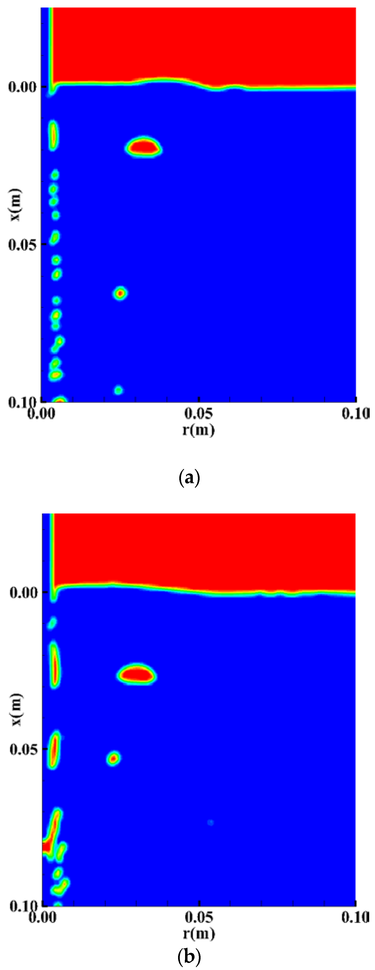
Surface phenomena of liquid jets into still water have been studied experimentally and numerically by many researchers [17,24]. Deformation of water column surface mainly depends on the water jet velocity, the pipe diameter, and surface tension. As the water jet is released by the circular nozzle, tiny disturbances appear on the jet flow surface. Subsequently, the shape of the water column surface becomes rougher and the jet water becomes finer and is bent into a helical shape during the falling process due to the increasing aerodynamic forces. Finally, a breakup phenomenon occurs after reaching a certain distance. However, the breakup of the water column did not appear in our research due to the smaller V0 and L1. Actually, the jet surface deformation phenomenon can be observed due to the surrounding air entrainment into the jet. The bubble breakup and coalescence become more and more relevant with the increasing air holdup below the surface, leading to a broad distribution of bubble sizes. Figure 6 shows the snapshots of computational AVF with different V0 for L1 = 0.025 m. It was found that the CLSVOF method was unable to capture the accurate deformation of air bubbles. However, the bubbly descending and ascending caused by the plunging jet can be observed clearly. The bubble size is determined by the balance between the surface tension forces and the inertial forces caused by the velocity changes. It is interesting to note that with increasing V0, the descending bubbles tend to be long and thin. However, the ascending bubble appears round in deep water, and it appears as a white cap shape near the water surface. As a result, V0 plays an unimportant role in the shape and size of ascending bubbles. A possible explanation is that the effect of jet velocity and momentum at the nozzle exit vanishes for the ascending bubbles, and their shape depends greatly on the buoyancy effect. The number of bubbles is far less than that from the experimental results, possibly due to the inability to capture the smaller bubbles and the neglect of bubble breakup and coalescence.
3.2. Jet Velocity Distribution
3.2.1. Mixture Velocity Distribution
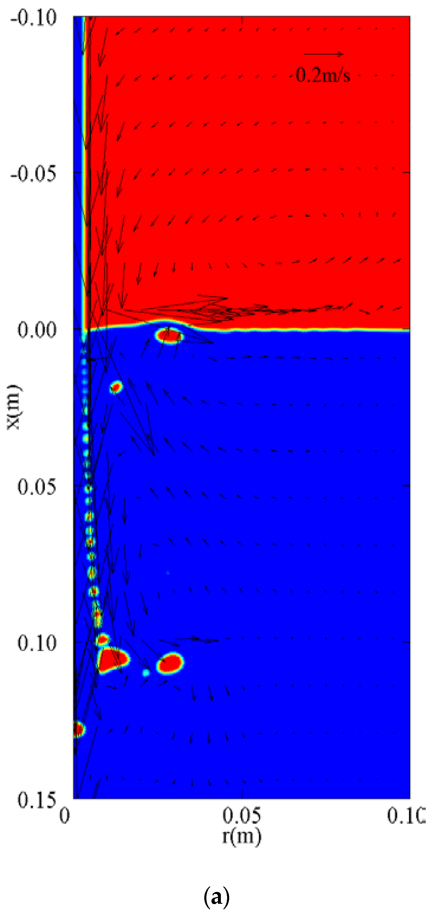
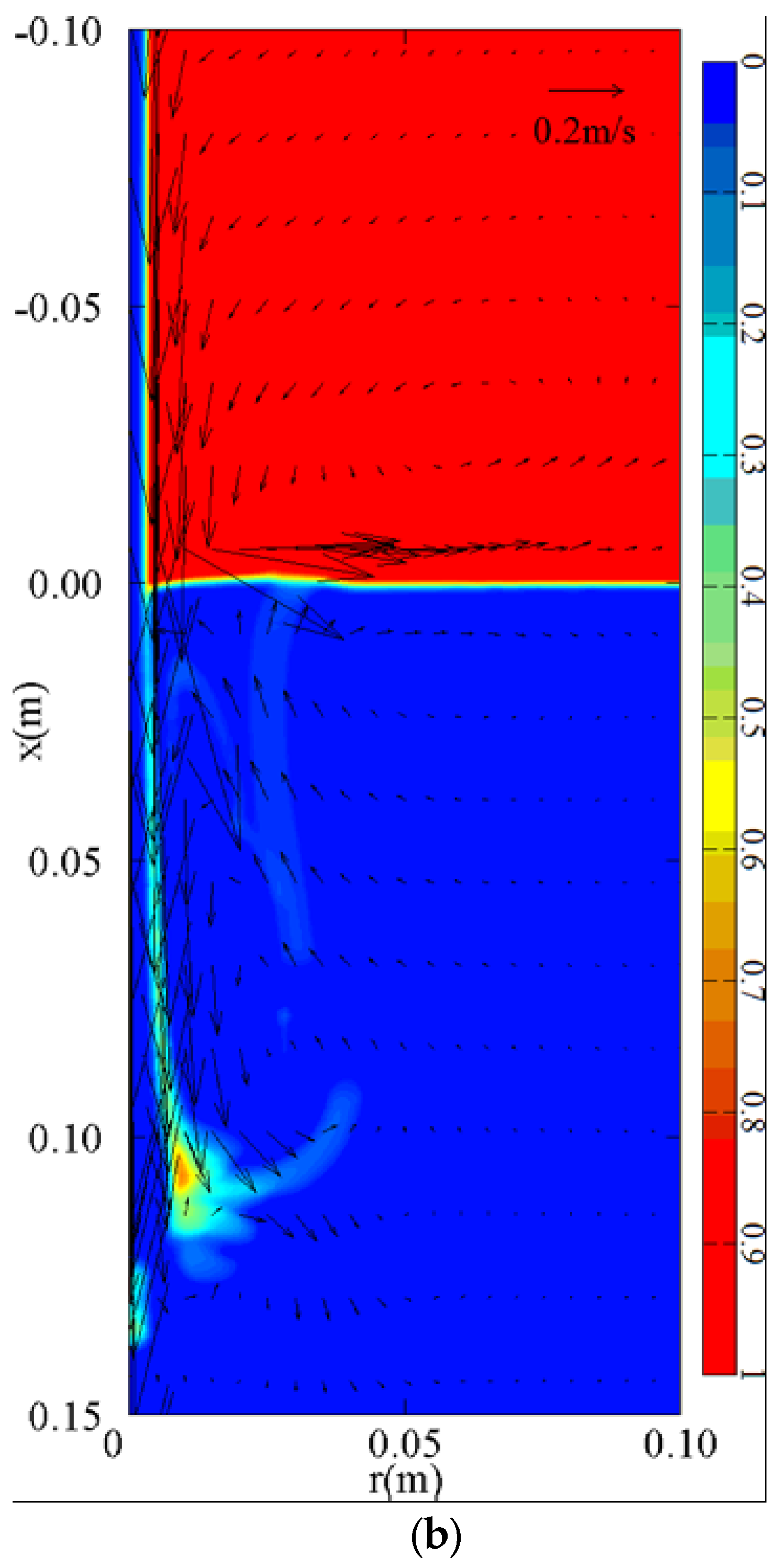
The velocity vector is a parameter including its magnitude and direction. Figure 7a shows a snapshot of the mixture velocity vectors and AVF, and Figure 7b indicates their time-averaged values. It was found that the flow structure basically comprises of two distinct regions below the impingement point: one is a diffusion cone with a downward flow motion induced by the plunging liquid jet, and the other is a swarm of rising bubbles which surrounds the diffusion cone, consistent with the trend reported by Chanson [3]. Obviously, there are two different directions of air flow in the diffusion region, one travels in the downward direction due to the entrainment of plunging jet and the other has an upward movement under the action of buoyancy. Many bubbles diffuse in the process of downward motion when the jet impulse is dissipated. This is different from the absence of entrainment bubbles at the jet centerline that occurs when using the Mixture method and the AVF contours that occurs when using the LS method, as reported by Qu et al. [15]. However, all methods produce a widening of the jets due to the viscous transport of vertical momentum and turbulent energy. A large number of ascending bubbles rise to the surface and escape, and the others are re-entrained on the centerline of the vertical jet. A large vortex occurs in the area from descending bubbles to ascending bubbles, mainly due to the coupling effect of jet momentum, gravity, and bubbly buoyancy, and the higher mixture velocities may be attributed to the turbulence generated by bubbles while they are approached.
3.2.2. Vertical Water Velocity Distribution at Centerline
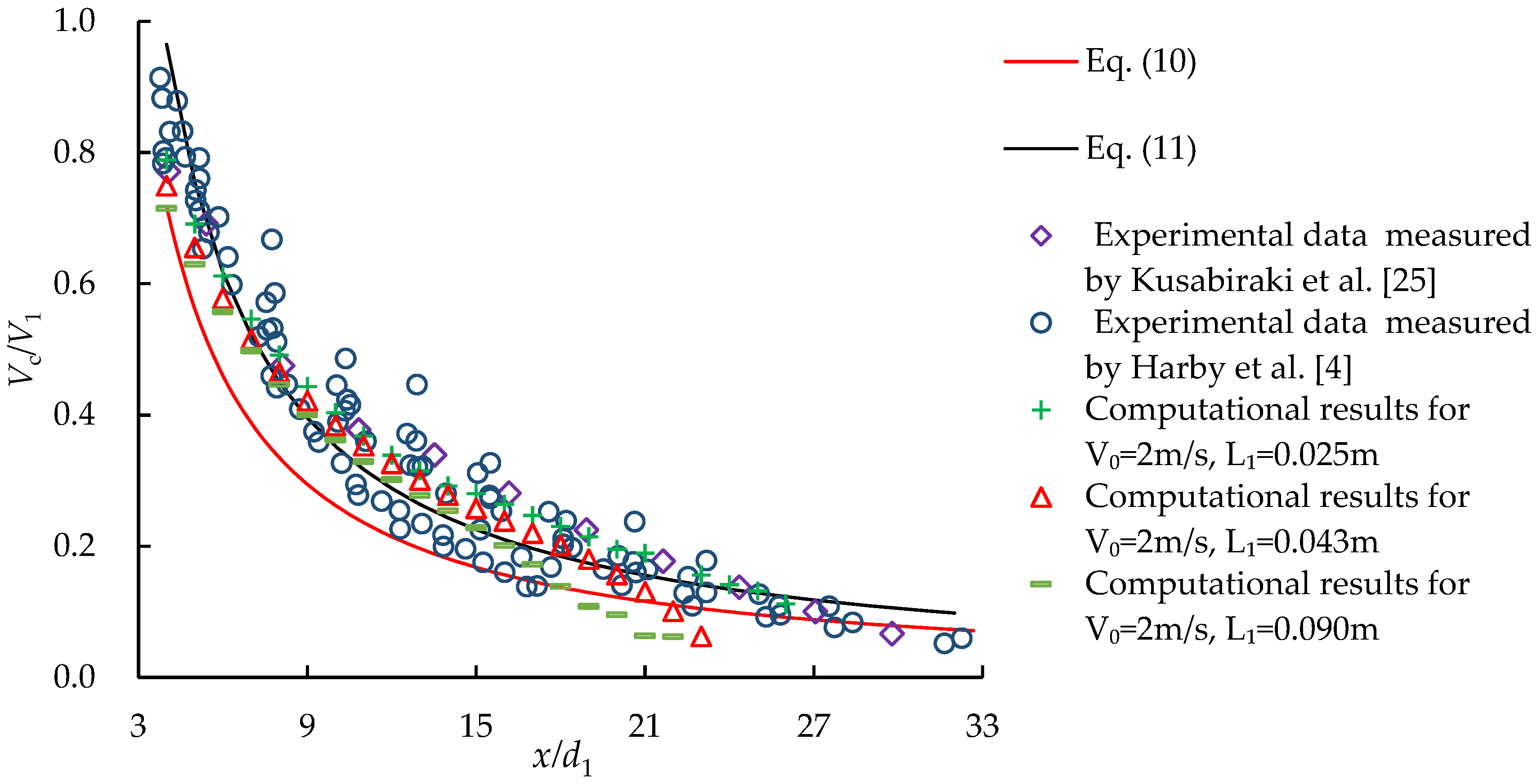
It is well known that Vc and Vr are significant parameters that are used to explore the hydraulic characteristic of a vertical plunging jet. McKeogh and Ervine [6] proposed a relationship between the decay ratio of vertical water velocity distribution at the centerline (Vc/V1) and x/d1, which ranged from about 3 to 20, for smooth plunging jets using a Pitot tube, as follows:
where d1 is the jet diameter at the impact point, and .
Figure 8 shows the variation of the computational Vc/V1 with x/d1 for the scenarios of V0 = 2 m/s and L1 = 0.025 m, 0.043 m, and 0.090 m, respectively. The figure compares the computational results with those from Equation (10) and the related experimental data reported by Harby et al. [4] and Kusabiraki et al. [25]. It was observed that the computational Vc/V1 obtained using the CLSVOF method and the experimental data reported by Harby et al. and Kusabiraki et al. were much higher than when using Equation (10), and Equation (10) underestimated 27% of the average relative deviation. Iguchi et al. [8] and Bin [26] also illustrated that Equation (10) does not agree well with the experimental data, and the reason, as explained by Bin [26], is that the tube is unable to precisely detect the liquid-phase velocity in the bubble dispersion region. In order to improve the accuracy of the Vc/V1 relationship with x/d1, a modified prediction equation was established using the data from the CLSVOF method as follows:
Its correlation coefficient was 0.94. Figure 8 shows that the average relative deviation between the experimental data reported by Harby et al. [4] and Kusabiraki [25] and Equation (11) is about 14.9%. Consequently, Equation (11) shows a certain degree of improvement over the existing Equation (10).
3.2.3. Radial Water Velocity Distribution
To investigate Vr for a round, single-phase turbulent jet, Chanson [27] measured the radial velocity distribution in the fully developed region and suggested the following empirical equation:
Note that Equation (12) is valid beyond the distance of 10d0 from the jet origin. Figure 9 shows the Vr/V1 relationship with r/d0 using Equation (12), the numerical results of the CLSVOF method, the LES-VOF method, the Mixture method, and the LS method reported by Khezzar et al. [13] and Qu et al. [15]. It was found that Vr/V1 has the maximum value at the jet centerline and gradually reduces to zero as it moves away from the centerline. Vr/V1 decreases with the increasing submerged depth, especially for a smaller r/d0. In addition, the differences in Vr/V1 for different submerged depth scenarios decreases with increasing r/d0. The reason for the discrepancies between numerical results and Equation (12) is that the latter is only valid for liquid-liquid jet flow. However, Vr/V1 of a plunging jet is affected obviously by the drag/buoyancy of entraining bubbles [15]. Furthermore, Vr/V1 in the centerline obtained by the LS and Mixture methods is higher than that obtained by Equation (12), but the CLSVOF and LES-VOF methods predict a lower value. A possible reason is that the jet central region is also affected by entrained bubbles for a plunging jet using the CLSVOF and LES-VOF methods; their drag/buoyancy effects aggravate the water disturbance and contribute greatly to the velocity decrease. As a result, the Vr of the plunging jet is smaller than that of the liquid-liquid jet in the advection and diffusion region. In addition, a set of experiments were performed by Harby et al. [4] on plunging water jets and a vertically submerged jet, demonstrating that the Vr of the plunging jet is also smaller than that of the liquid-liquid jet. Therefore, by using the same turbulence models and spatial discretization and different interface tracking methods reported by Qu et al. [15], the CLSVOF method predicted a more accurate and reasonable velocity than the Mixture and LS methods for a vertical plunging jet.
Figure 10 shows the dimensionless form of radial water velocity distribution Vr/Vc at sections x = 0.02 m, 0.04 m, 0.06 m, and 0.08 m for V0 = 2 m/s. Here, only two scenarios for L1 = 0.179 m and L1 = 0.141 m are shown due to their similar trends for all the scenarios. It was found that Vr/Vc approximately fits the Gaussian distribution, as follows:
where bw is the half-width of water velocity in the radial direction of the plunging jet, defined as the distance from the jet centerline to the location where Vr/Vc = 0.5. A similar Gaussian distribution of Vr/Vc was also found for vertical bubbly jets generated by injecting premixed gas and water into a water tank through a single-hole bottom nozzle [28]. However, there is a slight deviation in the vicinity of r/bw = 0.5, possibly due to the strong influence of entrained air bubbles.
3.3. AVF
To describe the AVF distribution for a vertical plunging jet, Chanson et al. [7] proposed the following empirical equation:
where C is the AVF, Qair is the air flow rate, Qw is the water flow rate of the plunging jet, D# is the dimensionless diffusivity of air bubbles, D# = 2Dt/(V0d0), Dt is the advection-diffusion coefficient, which considers the effects of turbulent dispersion and streamwise velocity gradient, I0 is the modified Bessel function of the first kind of order zero, and YCmax decides the radial location of the maximum AVF.
Figure 11 shows the mean AVF using the CLSVOF method, the LS method, and Equation (14) in the sections of x = 0.12 m, 0.13 m, and 0.14 m. It was found that the AVF peak locations obtained using the CLSVOF method are r = 0.003 m, 0.002 m, 0.002 m at the three different sections, respectively, while it is r = 0.003 m using the LS method at all three sections. The AVF obtained by the CLSVOF method was more consistent with Equation (14) than that of the LS method. Note that the AVF on the centerline using the CLSVOF method is not equal to zero, which is inconsistent with the LS method results. A possible explanation is that some entrained bubbles diffuse into the centerline location, while the jet impulse dissipates.
3.4. Turbulence Kinetic Energy (TKE)
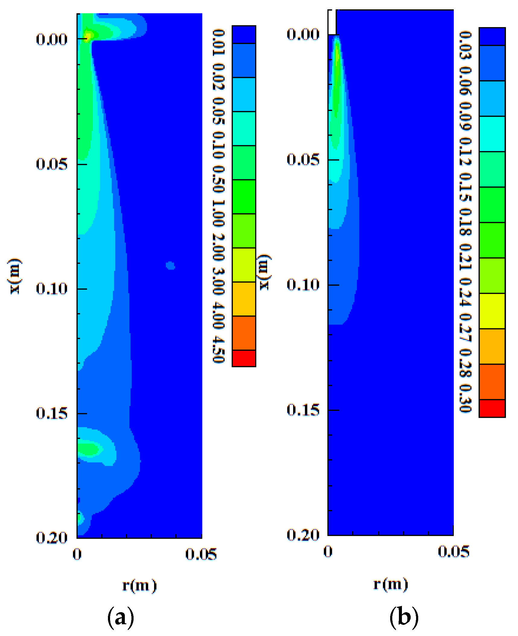
The distribution of TKE is shown in Figure 12a for L1 > 0 scenarios. It was found that the location of the maximum TKE is at the junction of the plunging jet and water surface, mainly due to a dramatic velocity change attributed to the obstruction of still water. However, the higher TKE appears at the higher velocity area below the water surface. In comparison with the plunging jet, Figure 12b shows the TKE of a submerged water jet for L1 = 0. It was found that the higher TKE occurs along the vertical extension line of the outer margin at the submerged jet boundary. With the increasing depth from the nozzle exit, the TKE increases dramatically and reaches its maximum value, then decreases.
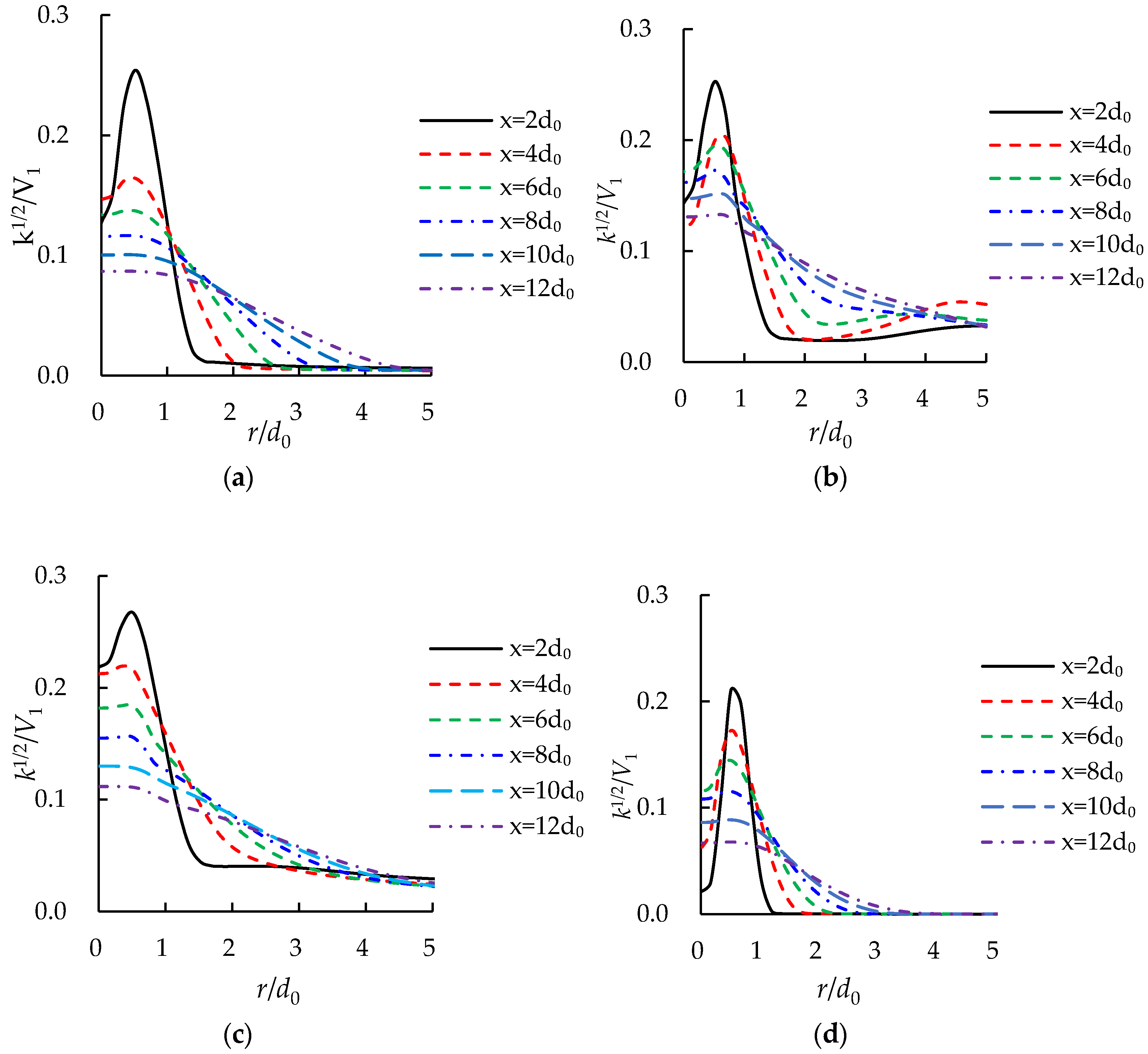
Figure 13 shows the k1/2/V1 distribution at various horizontal sections below the still water level. It was found that with increasing submerged depth, the maximum value of k1/2/V1 decreases. The present computational results show a trend consistent with the results of Khezzar et al. [13]. With the increase of relative radial distance r/d0 from 0, TKE first increases and then decreases for small submerged depth sections, such as x ≤ 6d0 in Figure 13a, x ≤ 10d0 in Figure 13b, x ≤ 8d0 in Figure 13c, and x ≤ 8d0 in Figure 13d. However, k1/2/V1 decreases with increasing r/d0 from 0 for a large submerged depth, such as x ≥ 8d0 in Figure 13a, x = 12d0 in Figure 13b, x ≥ 10d0 in Figure 13c, and x ≥ 10d0 in Figure 13d. Figure 13a,b show that TKE increases with increasing V0 for a constant L1 = 0.025 m to a large extent. At section x = 2d0, its peak value for V0 = 2 m/s increases from 0.29 m2/s2 to 0.432 m2/s2 for V0 = 2.5 m/s. At section x = 6d0, its peak value increases from 0.141 m2/s2 to 0.246 m2/s2. Figure 13a,d shows that k1/2/V1 of a plunging jet is obviously higher than that of a submerged jet for an equal V1 = 2.12 m/s due to the disturbance of entrainment air bubbles.
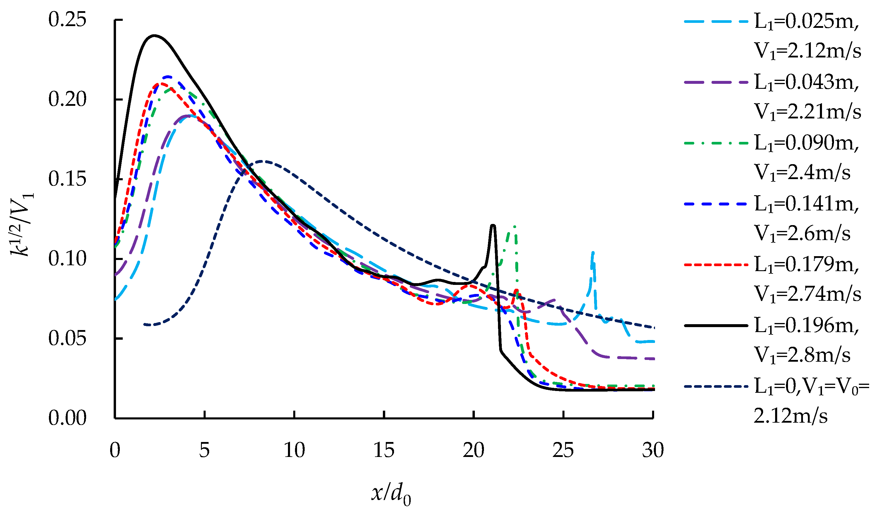
Figure 14 shows the k1/2/V1 distribution along the jet centerline. It was found that all the scenarios for plunging jets show a consistent trend. Specifically, k1/2/V1 increases rapidly to a maximum peak value near x/d0—from 2.8 to 4.5—and then decreases slowly. With the continual increase of x/d0, a second smaller peak occurs and then decreases to 0. The first peak of k1/2/V1 is because the jet impulse is greater than the resistance of still water, but it then decreases sharply due to the effect of the entrained bubbles’ buoyancy. The occurrence of the second peak is mainly attributed to the bubbles’ diffusion to the centerline after the jet momentum is scattered. In addition, it is interesting to note that the first peak nears the free water surface with increasing L1 and V1. For instance, when L1 increases from 0.025 m to 0.196 m, the location of the maximum peak changed from x = 4.5d0 to x = 2.5d0. Concerning the submerged jet, the TKE along the jet centerline increases rapidly to a peak value at about x = 8.5d0 and then decreases slowly. The location of the maximum TKE is farther from the water surface than the plunging jets for the same V1. In contrast, its second peak of TKE does not occur due to the absence of bubbly effects.
4. Conclusions
By using the CLSVOF method and the RANS approach, as well as the standard k-ε turbulence model, a 2-D axisymmetric mathematical model was used to investigate the hydraulic characteristic for a vertical plunging jet. The computational results were validated by comparison with the related experimental data reported by others, and they agreed well. The mathematical model was used to compute the distribution of hydraulic parameters, such as vertical water velocity, radial water velocity, AVF, and TKE, and their characteristics were also examined. The computational results showed that the velocity at the nozzle exit plays an unimportant role in the shape and size of ascending bubbles. The radial mean water velocity has a maximum value at the jet centerline. The AVF values using the CLSVOF method are more consistent with the related empirical equation than with that obtained using the LS method. The maximum TKE occurs near the water surface for a plunging jet. However, the higher TKE occurs along the vertical extension line of the outer margin at the jet boundary for a submerged jet. With the increasing submerged depth, the TKE increases dramatically to reach its maximum value and then decreases. For an equal impacting velocity at the impingement point, the TKE of a plunging jet is higher than that of a submerged jet. With the increase of relative radial distance from the centerline, the TKE first increases and then decreases at a smaller submerged depth section; however, it continues to decrease at a larger submerged depth section.
The limitations of this study should be pointed out. First, the numerical AVF and TKE values were not compared with the related experimental data, and the mathematical model using the CLSVOF method needs further validation to extend its applicability to an engineering case. In addition, it neglected the complex behavioral effects of entrained bubbles, such as their breakup and coalescence on the hydrodynamic characteristic. This should be considered in future work.
Author Contributions
Z.Y. designed the study and wrote the manuscript, Q.J., Y.L. and Y.W. participated in the numerical simulations, D.Y. prepared figures. All authors reviewed the manuscript.
Funding
The study is financed by National Natural Science Foundation of China (Grant No. 51579229), The Key Research and Development Plan of Shandong Province, China (Grant No. 2017GHY15103) and State Key Laboratory of Ocean Engineering, China (Grant No. 1602).
Acknowledgments
The authors would like to thank the Reviewers and the Assistant Editor for providing valuable comments that helped in improving the overall quality of the manuscript.
Conflicts of Interest
The authors declare no conflict of interest. The sponsors had no role in the design of the study; in the collection, analyses, or interpretation of data; in the writing of the manuscript, and in the decision to publish the results.
List of Symbols
| bw | half-width of water velocity | (m) |
| C | air void fraction | (-) |
| d0 | nozzle exit diameter | (m) |
| d1 | diameter at the impact point | (m) |
| D# | dimensionless diffusivity of air bubbles | (-) |
| Dt | advection diffusion coefficient | (-) |
| F | VOF function | (-) |
| Fr | Froude number | (-) |
| gravity acceleration | (m/s2) | |
| H | Heaviside function | (-) |
| Hp | penetration depth | (m) |
| I | turbulent intensity at the nozzle exit | (-) |
| I0 | modified Bessel function | (-) |
| K | turbulence kinetic energy | (m2/s2) |
| l | local mean interface curvature | (m−1) |
| L1 | distance from the nozzle exit to the still liquid surface | (m) |
| Qair | air flow rate | (L/min) |
| Qw | water flow rate of plunging jet | (L/min) |
| r | radial distance from the vertical centreline | (m) |
| mixture velocity | (m/s) | |
| V0 | velocity at the nozzle exit | (m/s) |
| V1 | impacting velocity at impingement point | (m/s) |
| Vc | water velocity at the centreline | (m/s) |
| Vr | water velocity in the radial direction | (m/s) |
| x | the vertical distance measured from the still water level | (m) |
| μ | dynamic viscosity coefficient | (kg/(m·s)) |
| ρ | mixture density | (kg/m3) |
| ϕ | LS function | (-) |
| ν | kinematic viscosity of water | (m2s−1) |
References
- Goldring, B.T.; Mawer, W.T.; Thomas, N. Level surges in the circulating water downshaft of large generating stations. In Proceedings of the 3rd International Conference on Pressure Surges, Canterbury, UK, 25–27 March 1980. [Google Scholar]
- Robison, R. Chicago’s waterfalls. Civ. Eng. 1994, 64, 36. [Google Scholar]
- Chanson, H. Air Bubble Entrainment in Free-Surface Turbulent Shear Flows; Academic Press: London, UK, 1996. [Google Scholar]
- Harby, K.; Chiva, S.; Muñoz-Cobo, J.L. An experimental study on bubble entrainment and flow characteristics of vertical plunging water jets. Exp. Therm. Fluid Sci. 2014, 57, 207–220. [Google Scholar] [CrossRef]
- Qu, X.; Goharzadeh, A.; Khezzar, L.; Molki, A. Experimental characterization of air-entrainment in a plunging jet. Exp. Therm. Fluid Sci. 2013, 44, 51–61. [Google Scholar] [CrossRef]
- McKeogh, E.J.; Ervine, D.A. Air entrainment rate and diffusion pattern of plunging liquid jets. Chem. Eng. Sci. 1981, 36, 1161–1172. [Google Scholar] [CrossRef]
- Chanson, H.; Aoki, S.; Hoque, A. Physical modelling and similitude of air bubble entrainment at vertical circular plunging jets. Chem. Eng. Sci. 2004, 59, 747–758. [Google Scholar] [CrossRef] [Green Version]
- Iguchi, M.; Okita, K.; Yamamoto, F. Mean velocity and turbulence characteristics of water flow in the bubble dispersion region induced by plunging water jet. Int. J. Multiph. Flow 1998, 24, 523–537. [Google Scholar] [CrossRef]
- Suciu, G.D.; Smigelschi, O. Size of the submerged biphasic region in plunging jet systems. Chem. Eng. Sci. 1976, 31, 1217–1220. [Google Scholar] [CrossRef]
- Cumming, I.W. The Impact of Failing Liquids with Liquid Surfaces. Ph.D. Thesis, Loughborough University of Technology, Loughborough, UK, 1975. [Google Scholar]
- Lopes, P.; Tabor, G.; Carvalho, R.F.; Leandro, J. Explicit calculation of natural aeration using a Volume-of-Fluid model. Appl. Math. Model. 2016, 40, 7504–7515. [Google Scholar] [CrossRef] [Green Version]
- Deshpande, S.S.; Trujillo, M.F. Distinguishing features of shallow angle plunging jets. Phys. Fluids 2013, 25, 082103. [Google Scholar] [CrossRef]
- Khezzar, L.; Kharoua, N.; Kiger, K.T. Large eddy simulation of rough and smooth liquid plunging jet processes. Prog. Nucl. Energy 2015, 85, 140–155. [Google Scholar] [CrossRef]
- Shonibare, O.Y.; Wardle, K.E. Numerical Investigation of Vertical Plunging Jet Using a Hybrid Multifluid–VOF Multiphase CFD Solver. Int. J. Chem. Eng. 2015, 14. [Google Scholar] [CrossRef]
- Qu, X.L.; Khezzar, L.; Danciu, D.; Labois, M.; Lakehal, D. Characterization of plunging liquid jets: A combined experimental and numerical investigation. Int. J. Multiph. Flow 2011, 37, 722–731. [Google Scholar] [CrossRef]
- Olsson, E.; Kreiss, G.; Zahedi, S. A conservative level set method for two phase flow II. J. Comput. Phys. 2007, 225, 785–807. [Google Scholar] [CrossRef]
- Xiao, F.; Dianat, M.; McGuirk, J.J. LES of turbulent liquid jet primary breakup in turbulent coaxial air flow. Int. J. Multiph. Flow 2014, 60, 103–118. [Google Scholar] [CrossRef] [Green Version]
- Patankar, S. Numerical Heat Transfer and Fluid Flow; CRC Press: Boca Raton, FL, USA, 1980. [Google Scholar]
- Van Doormaal, J.P.; Raithby, G.D. Enhancements of the SIMPLE method for predicting incompressible fluid flows. Numer. Heat Transf. 1984, 7, 147–163. [Google Scholar] [CrossRef]
- Richardson, L.F.; Gaunt, J.A. The deferred approach to the limit. Part, I. Single lattice. Part II. Interpenetrating lattices. Philos. Trans. R. Soc. Lond. Ser. A Contain. Pap. Math. Phys. Character 1927, 226, 299–361. [Google Scholar] [CrossRef]
- Ferziger, J.H.; Perić, M. Further discussion of numerical errors in CFD. Int. J. Numer. Methods Fluids 1996, 23, 1263–1274. [Google Scholar] [CrossRef]
- Broadhead, B.L.; Rearden, B.T.; Hopper, C.M.; Wagschal, J.J.; Parks, C.V. Sensitivity-and uncertainty-based criticality safety validation techniques. Nucl. Sci. Eng. 2004, 146, 340–366. [Google Scholar] [CrossRef]
- Celik, I.B.; Ghia, U.; Roache, P.J. Procedure for estimation and reporting of uncertainty due to discretization in CFD applications. J. Fluids Eng. 2008, 130, 078001. [Google Scholar]
- Ma, Y.; Zhu, D.Z.; Rajaratnam, N.; Camino, G.A. Experimental study of the breakup of a free-falling turbulent water jet in air. J. Hydraul. Eng. 2016, 142, 06016014. [Google Scholar] [CrossRef]
- Kusabiraki, D.; Murota, M.; Ohno, S.; Yamagiwa, K.; Yasuda, M.; Ohkawa, A. Gas entrainment rate and flow pattern in a plunging liquid jet aeration system using inclined nozzles. J. Chem. Eng. Jpn. 1990, 23, 704–710. [Google Scholar] [CrossRef]
- Bin, A.K. Gas entrainment by plunging liquid jets. Chem. Eng. Sci. 1993, 48, 3585–3630. [Google Scholar] [CrossRef]
- Chanson, H. Environmental Hydraulics for Open Channel Flows; Butterworth-Heinemann: Oxford, UK, 2004. [Google Scholar]
- Neto, I.E.L.; Zhu, D.Z.; Rajaratnam, N. Bubbly jets in stagnant water. Int. J. Multiph. Flow 2008, 34, 1130–1141. [Google Scholar] [CrossRef]
Figure 1.
A schematic of the computational domain.

Figure 2.
The flowchart of the CLSVOF method.

Figure 3.
The computational results using different grids of (a) Vr/V0 at section x = 2d0 and of (b) Vc/V0 for V0 = 0.63 m/s and L1 = 0.012 m.
Figure 3.
The computational results using different grids of (a) Vr/V0 at section x = 2d0 and of (b) Vc/V0 for V0 = 0.63 m/s and L1 = 0.012 m.

Figure 4.
The Hp/L1 relationship with V1/V0, obtained by comparing data from the CLSVOF method to experimental data reported by Qu et al. [15].
Figure 4.
The Hp/L1 relationship with V1/V0, obtained by comparing data from the CLSVOF method to experimental data reported by Qu et al. [15].

Figure 5.
The computational results in comparison to experimental data reported by Qu et al. [5] for (a) the Vr/V0 relationship with r/d0 for different submerged depth scenarios, and (b) the Vc/V1 relationship with x/L1 for V0 = 0.63 m/s and L1 = 0.012 m.
Figure 5.
The computational results in comparison to experimental data reported by Qu et al. [5] for (a) the Vr/V0 relationship with r/d0 for different submerged depth scenarios, and (b) the Vc/V1 relationship with x/L1 for V0 = 0.63 m/s and L1 = 0.012 m.

Figure 6.
The jet bubbles and free surface deformation snapshots for (a) V0 = 2.5 m/s and L1 = 0.025 m, (b) V0 = 3 m/s and L1 = 0.025 m.
Figure 6.
The jet bubbles and free surface deformation snapshots for (a) V0 = 2.5 m/s and L1 = 0.025 m, (b) V0 = 3 m/s and L1 = 0.025 m.

Figure 7.
The mixture velocity vectors and AVF contours for V0 = 2 m/s and L1 = 0.141 m of (a) snapshot and (b) time-averaged values.
Figure 7.
The mixture velocity vectors and AVF contours for V0 = 2 m/s and L1 = 0.141 m of (a) snapshot and (b) time-averaged values.


Figure 8.
The comparison of Vc/V1 values obtained from computational results, Equations (10) and (11), and experimental data reported by Kusabiraki et al. [15] and Harby et al. [4].

Figure 9.
The Vr/V1 relationship with r/d0 for V0 = 2 m/s and L1 = 0.025 m using Equation (12) and the LS, Mixture, CLSVOF, and LES-VOF methods at the sections of (a) x = 0.05 m, (b) x = 0.06 m, and (c) x = 0.07 m.
Figure 9.
The Vr/V1 relationship with r/d0 for V0 = 2 m/s and L1 = 0.025 m using Equation (12) and the LS, Mixture, CLSVOF, and LES-VOF methods at the sections of (a) x = 0.05 m, (b) x = 0.06 m, and (c) x = 0.07 m.

Figure 10.
The computational Vr/Vc relationship with r/bw for V0 = 2 m/s and (a) L1 = 0.196 m and (b) L1 = 0.141 m.
Figure 10.
The computational Vr/Vc relationship with r/bw for V0 = 2 m/s and (a) L1 = 0.196 m and (b) L1 = 0.141 m.

Figure 11.
The computational average AVF using the LS and CLSVOF methods with Equation (14) for V1 = 2.12 m/s and L1 = 0.025 m at (a) x = 0.12 m, (b) x = 0.13 m, and (c) x = 0.14 m.
Figure 11.
The computational average AVF using the LS and CLSVOF methods with Equation (14) for V1 = 2.12 m/s and L1 = 0.025 m at (a) x = 0.12 m, (b) x = 0.13 m, and (c) x = 0.14 m.


Figure 12.
The TKE (m2/s2) distribution for (a) a plunging jet with V0 = 2 m/s, L1 = 0.025 m (V1 = 2.12 m/s) and (b) a submerged jet with V0 = 2.12 m/s, L1 = 0 m (V1 = 2.12 m/s).
Figure 12.
The TKE (m2/s2) distribution for (a) a plunging jet with V0 = 2 m/s, L1 = 0.025 m (V1 = 2.12 m/s) and (b) a submerged jet with V0 = 2.12 m/s, L1 = 0 m (V1 = 2.12 m/s).

Figure 13.
The k1/2/V1 relationship with r/d0 at different submerged depth sections for (a) a plunging jet at V0 = 2 m/s, L1 = 0.025 m (V1 = 2.12 m/s), (b) a plunging jet at V0 = 2.5 m/s, L1 = 0.025m (V1 = 2.60 m/s), (c) a plunging jet at V0 = 2 m/s, L1 = 0.179 m (V1 = 2.74 m/s), and (d) a submerged jet at V0 = 2.12 m/s, L1 = 0 m(V1 = 2.12 m/s).

Figure 14.
The TKE along the jet centerline with V0 = 2 m/s for different L1.


Table 1.
The analysis of discretization error.
| Grid | At the Jet Centerline of Section x = 2d0 for V0 = 0.63 m/s and L1 = 0.012 m | ||
|---|---|---|---|
| Grid Partition | Total Grids Number | Grid Size (m) | Water Velocity (m/s) |
| Grid 1 | 10,950 | 0.002 | 0.4692 |
| Grid 2 | 43,800 | 0.001 | 0.7841 |
| Grid 3 | 175,200 | 0.0005 | 0.7523 |
| Extrapolated values | 0.7487 | ||
| Extrapolated relative error | 0.5% | ||
| Grid convergence index | 0.6% | ||
© 2018 by the authors. Licensee MDPI, Basel, Switzerland. This article is an open access article distributed under the terms and conditions of the Creative Commons Attribution (CC BY) license (http://creativecommons.org/licenses/by/4.0/).
Share and Cite
MDPI and ACS Style
Yin, Z.; Jia, Q.; Li, Y.; Wang, Y.; Yang, D. Computational Study of a Vertical Plunging Jet into Still Water. Water 2018, 10, 989. https://doi.org/10.3390/w10080989
AMA Style
Yin Z, Jia Q, Li Y, Wang Y, Yang D. Computational Study of a Vertical Plunging Jet into Still Water. Water. 2018; 10(8):989. https://doi.org/10.3390/w10080989
Chicago/Turabian StyleYin, Zegao, Qianqian Jia, Yuan Li, Yanxu Wang, and Dejun Yang. 2018. "Computational Study of a Vertical Plunging Jet into Still Water" Water 10, no. 8: 989. https://doi.org/10.3390/w10080989
Note that from the first issue of 2016, this journal uses article numbers instead of page numbers. See further details here.