Assessment of Local Climate Change: Historical Trends and RCM Multi-Model Projections Over the Salento Area (Italy)


Department of Engineering and Architecture, University of Parma, 43124 Parma, Italy
*
Author to whom correspondence should be addressed.
Water 2018, 10(8), 978; https://doi.org/10.3390/w10080978
Submission received: 28 June 2018
/
Revised: 18 July 2018
/
Accepted: 23 July 2018
/
Published: 25 July 2018
(This article belongs to the Section Hydrology)
Abstract
:This study provides an up-to-date analysis of climate change over the Salento area (southeast Italy) using both historical data and multi-model projections of Regional Climate Models (RCMs). The accumulated anomalies of monthly precipitation and temperature records were analyzed and the trends in the climate variables were identified and quantified for two historical periods. The precipitation trends are in almost all cases not significant while the temperature shows statistically significant increasing tendencies especially in summer. A clear changing point around the 80s and at the end of the 90s was identified by the accumulated anomalies of the minimum and maximum temperature, respectively. The gradual increase of the temperature over the area is confirmed by the climate model projections, at short—(2016–2035), medium—(2046–2065) and long-term (2081–2100), provided by an ensemble of 13 RCMs, under two Representative Concentration Pathways (RCP4.5 and RCP8.5). All the models agree that the mean temperature will rise over this century, with the highest increases in the warm season. The total annual rainfall is not expected to significantly vary in the future although systematic changes are present in some months: a decrease in April and July and an increase in November. The daily temperature projections of the RCMs were used to identify potential variations in the characteristics of the heat waves; an increase of their frequency is expected over this century.
1. Introduction
Climate change is a matter of many debates in the scientific community and describes the perturbations of the climate system due to weather pattern changes. Over the past 150 years, we observed extremely rapid changes in climate that cannot be ascribed to the same natural processes that generated past variations. According to the Fifth Assessment Report (AR5) of the Intergovernmental Panel on Climate Change (IPCC, [1]) the primary causes of global warming are related to human activities and, in particular, to the emission of greenhouse gases. Adaptation and mitigation strategies to reduce these emissions are required and are currently underway in many countries. The goal set during the 21st session of the Conference of the Parties (COP21) to the United Nations Framework Convention on Climate Change (UNFCCC, [2]), is to limit global warming to below 2 °C above pre-industrial levels and pursuing efforts to limit the temperature increase to 1.5 °C.
The present study focuses on the Salento area, in the Apulia Region, southeast Italy, where two of the main economic sectors, tourism and agriculture (especially olive oil and wine production), could be affected by climate change. Salento is part of the Mediterranean basin identified by Giorgi [3] as one of the most responsive regions to climate change (Hot-Spots). Philandras et al. [4] showed that the majority of the Mediterranean regions (with few exceptions) have experienced negative trends of the annual precipitation totals (in the period 1901–2009) and a decrease of about 20% in the annual number of rainy days. According to the Italian National Institute for Environmental Protection and Research (ISPRA, [5]), in Italy the 21st century mean temperature anomalies, with respect to the period 1961–1990, are on average higher than the global land ones; the mean temperature trend in the period 1981–2016 was equal to +0.36 °C/decade.
Besides the analysis of long-term observed precipitation and temperature time-series, one of the most recognized approaches to make future projections, is to adopt physically-based climate model data that account for different greenhouse emission scenarios. General Circulation Models (GCMs) are very helpful in understanding the future evolution of the global climate, but have a spatial resolution (100–300 km) too coarse for assessing regional or local changes [6]. To get a better spatial resolution (10–50 km), Regional Climate Models (RCMs) are obtained by dynamically downscaling GCM data [7]. However, these models are unable to accurately reproduce the historical climate since they suffer systematic biases [8] in the simulated variables (e.g., precipitation and temperature); a correction is therefore needed to obtain reliable local scale results [9]. Another issue is related to the quantification of the inherent uncertainty of the climate models; the reliability of the future projections can be investigated studying their variability with a multi-model ensemble of data: different combinations of GCMs, RCMs and emission scenarios [9,10].
Alpert et al. [11], using RCM data, found that the average temperature over the Eastern Mediterranean area has increased by 1.5 ÷ 4 °C in the last 100 years and the precipitation has exhibited a negative trend in the last 50 years. Future climate projections for the 21st century over the Mediterranean basin are analyzed in different studies based on GCMs and RCMs (e.g., [12,13,14]). The results, according to different model projections and emission scenarios, globally show an increase in temperature in all seasons and for all parts of the Mediterranean, with maximum positive increments in summer; a pronounced decrease in precipitation is projected, especially for the warm season (with few exceptions). Fine scale structures in the precipitation signal, induced by the local orography, are not caught by the GCM projections but are present in the RCM ones [12]. The extremes in temperature and the frequency of the heat waves are also expected to increase over the Mediterranean area (e.g., Zittis et al. [15]), although their characteristics and effects on human health are not uniform and are related to the local climate and the population tolerance [16]. ISPRA analyzed the future climate in Italy [17] using four RCMs. The climate model data were part of the Med-CORDEX project [18] and developed according to two of the most recent emission scenarios adopted by the IPCC in AR5: the Representative Concentration Pathways (RCPs), RCP4.5 and RCP8.5. The grid resolution was of 0.44° (~50 km) and no bias correction of the RCM data was performed. Precipitation and temperature were evaluated in three future periods, 2021–2050, 2041–2070 and 2061–2090, as anomalies with respect to the 1971–2000 RCM projections (reference period). According to the ensemble mean, temperature will rise in the whole nation with a moderate spatial variation; under the RCP4.5, increments between 1.25 °C and 1.75 °C are estimated in the period 2021–2050, from 1.75 °C to 2.25 °C at 2041–2070 and from 2.0 °C to 2.5 °C at 2061–2090. With the RCP8.5 the temperature increases from 1.5 °C to 2.0 °C in the first period, from 2.75 °C to 3.25 °C in the second period and from 3.75 °C to 4.5 °C in the last period. Looking at the individual models, a higher heterogeneity (with respect to the ensemble mean) is observed over the national territory. This suggests, for local studies, the use of a larger ensemble of models, with a higher spatial resolution, to better identify the potential changes and quantify the uncertainty in the results. Precipitation data show a higher spatial variability between models and over Italy; in southeast Italy, according to the ensemble mean, the models show a decrease in the annual rainfall below 50 mm in almost all periods and for both scenarios, with the exception of the period 2061–2090 under the RCP4.5 when increments (<50 mm) are found.
At local scale, Kapur et al. [19] analyzed the climate change in the Apulia region, studying historical precipitation and temperature records available at 162 meteorological stations in the period 1950–1990; the observed time-series were extended until 2100 based on the GCM HadCM3, developed by the Hadley Centre for Climate Prediction and Research (UK). The results show an increase of temperature in the range 1.3 ÷ 2.5 °C over the 21st century and a non-significant change of precipitation on a yearly basis, with a slight decrease in the summer months and a small increase in the winter season. Later, the study of Lionello et al. [20] investigated the precipitation and temperature records for the Apulia region in the historical period 1951–2005 and analyzed their possible variations for the future (until 2050). Temperature trends were calculated for the time series recorded at 11 gauges for the whole available historical period and the shorter time interval 1976–2005. The Mann Kendall test [21,22] was used to assess the trend significance and the Theil-Sen estimator [23] to quantify its linear slope. At annual scale, the minimum temperature has increased at a rate of 0.18 °C/decade in the period 1951–2005 and 0.45 °C/decade in the period 1976–2005, with maximum rates during the warm season. Maximum temperature does not show significant variations in the period 1951–2005 but presents an increase of 0.47 °C/decade in the period 1976–2005. Precipitation trends were evaluated for the period 1951–2005 at 15 rain gauges; trends were not statistically significant (90% confidence level) for all months. At annual scale, the Authors found a total precipitation decrease (statistically significant) at a rate of 14.9 mm/decade. Future climate projections were based on seven RCMs developed in the European project ENSEMBLES [24] and on three RCMs of the CIRCE project [25], with resolution from about 25 km to about 80 km. All simulations were based on the A1B emission scenario, one of those reported in the Special Report on Emissions Scenarios (SRES, [26]) and used in the Fourth Assessment Report (AR4) of the IPCC [27]. The climate models estimate, for the study area, a temperature increase of about 2 °C by 2050 with respect to the period 1961–1990; annual, minimum and maximum daily temperatures are expected to increase with rates between 0.35 °C/decade and 0.6 °C/decade (period 2001–2050). A small decrease of annual precipitation (about 10 mm/decade) is evaluated at 2050 with a high inter-annual variability.
The aim of this work is to provide a valuable and up-to-date analysis of the past, present and future climate variability for the Salento area (south of the Apulia region), which will be useful as guide to think and plan mitigation and adaptation strategies. The study starts with the examination of the historical precipitation and temperature data in the last 80 years (updated to 2012) by means of trend analyses (at monthly and annual scale and with different time windows). The accumulated anomalies were used to identify changing points in the recorded time-series. We then used the data of 13 high-resolution RCMs based on two of the most recent emission scenarios (RCP4.5 and RCP8.5) to assess the potential effects of climate change over the Salento area until 2100; the same data were used to identify any future changes in the characteristics of the heat waves. This paper is organized as follows: Section 2 introduces the study area, describes the available historical and climate model data and discusses the methods. Section 3 presents and discusses the main results of the study while conclusions are presented in Section 4.
2. Materials and Methods
2.1. Study Area and Available Data
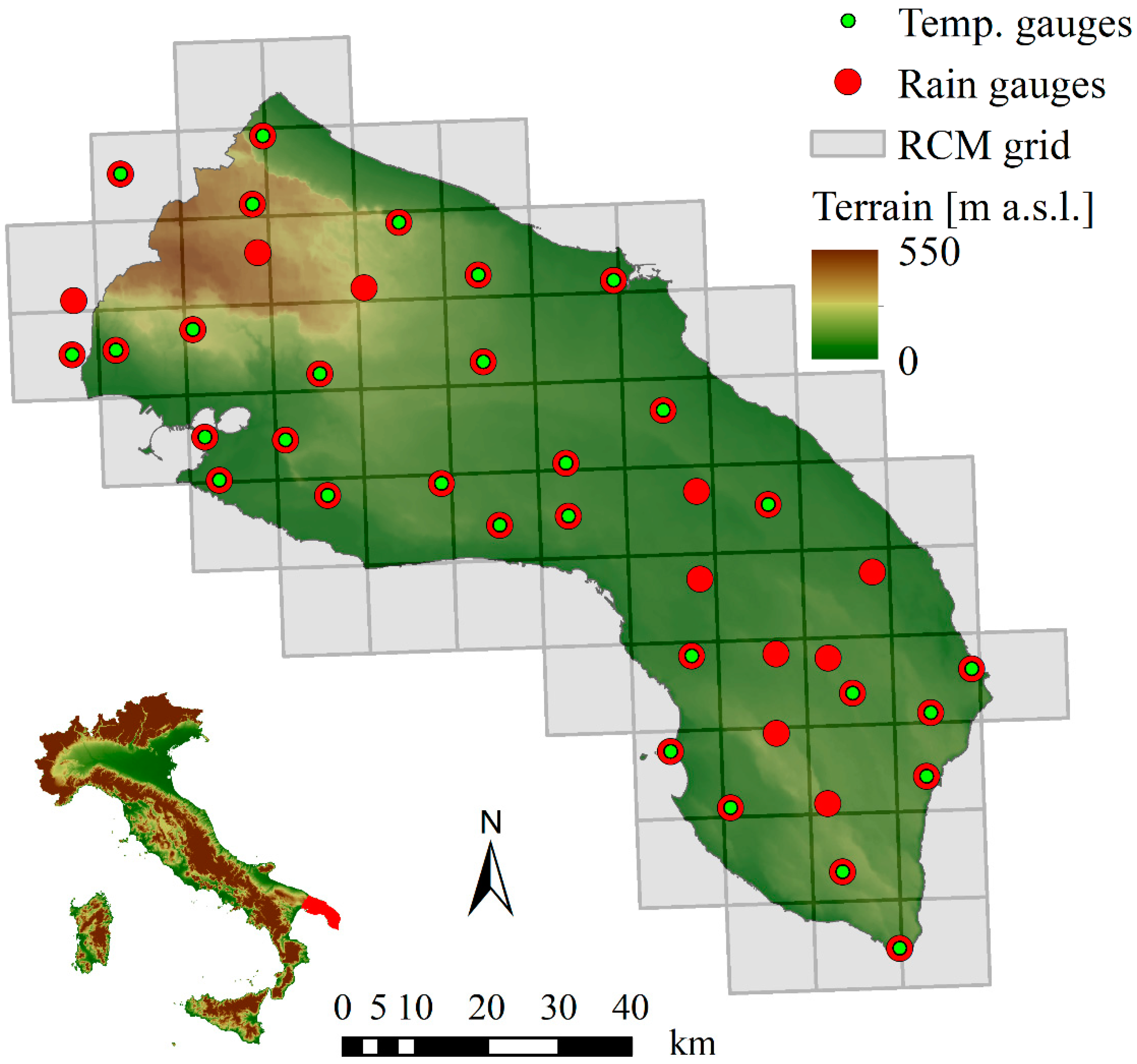
In this study, we analyzed the historical and future climate data in the Salento area, a portion of the Apulia region, in southeast Italy (Figure 1). Salento is a peninsula bordered by the Ionian Sea to the west and the Adriatic Sea to the south and east. The area covers about 6200 km2 with a perimeter of about 800 km, of which 700 km is coastline. The investigated domain is almost flat, with few gentle hills in the northwest border; the average elevation is about 100 m a.s.l. and the climate is Mediterranean with hot and dry summers and mild, wet winters. The average (1933–2012) mean temperature is about 16.5 °C, the coldest months are January and February, with an average mean temperature of about 9 °C and an average minimum temperature of about 5.5 °C, while the warmer months are July and August with an average mean temperature of about 25.4 °C and an average maximum temperature of about 30.7 °C. The average (1933–2012) annual precipitation is about 650 mm; the rainfall is concentrated in the autumn-winter months (about 70% of the total), with a high inter-annual variability. Agriculture is one of the primary segments of the Salento economy, together with tourism, mainly during summer; both the sectors strongly depend on the climate.
The historical climate data were extracted from a public regional database (www.protezionecivile.puglia.it) for 40 rain and 30 temperature gauges within and surrounding the Salento area. For these stations, the number of rainy days and the precipitation totals were available at monthly scale, together with the monthly maximum, minimum and mean temperature. From this network, we selected 30 rain and 18 temperature stations that had a long period of records (1933–2012), reliable data and a number of missing values less than 30%. Figure 1 depicts the chosen gauging stations, which are almost uniformly distributed over the study area and located to an altitude ranging from 15 m a.s.l. to 420 m a.s.l.
To analyze the future climate over the study area, daily precipitation and mean temperature data were extracted from 13 RCMs, combined with different GCMs (Table 1), of the EURO-CORDEX ensemble [28]. All the chosen climate models have a grid resolution of 0.11° (grid EUR-11, 12.5 km), in part depicted in Figure 1. Data are available for a historical simulation from 1950/1970 to 2005 and a scenario run from 2006 to 2100; the future projections were based on two Representative Concentration Pathways (RCPs): RCP4.5 and RCP8.5.
2.2. Analysis of the Historical Data
The precipitation and temperature data, selected from the available gauging stations (Figure 1), were used to identify changing points and trends in the recorded time-series. Before performing these analyses, the gaps in the data set were filled by means of the records available in the station that best matches (based on the Pearson correlation coefficient) the missing site data, using a linear regression approach [29].
After the data integration, we proceeded with the computation of the accumulated anomalies [30] with the aim of capturing potential changing points in both the precipitation and temperature historical records. The accumulated anomaly at time t, , of the generic series was calculated as:
where is the mean of . In this work, the anomalies were evaluated at monthly scale, so is month-dependent.
The Mann-Kendall test [21,22] was applied to identify the presence of trends in the time series at the 5% significance level. It is a non-parametric test, independent from the data distribution, used to detect the presence of monotonic trends. The correction recommended by Hamed and Rao [31] was applied to compensate the data serial correlation, which can affect the test results. The magnitude of the trend was quantified by the Theil-Sen estimator [23], also a non-parametric method, which is less sensitive to outliers than the simple linear regression model.
All the analyses were performed, at monthly and annual scale, at each gauging station location. In addition, we considered the averaged climate variables over the study area, estimated using the Thiessen polygon method.
2.3. Analysis of the Climate Model Data
As reported in Section 2.1, for this study we made use of an ensemble of 13 RCM simulations with daily climate data available over a grid with resolution of 0.11° (grid EUR-11, 12.5 km). As already mentioned before, RCM data may require the correction of systematic errors (bias correction); this is usually done with reference to a historical period (control period) for which observed and modeled time-series are available. The same correction factors identified in the control period are then assumed to hold for the future. Different methodologies are presented in literature for the bias correction of climate variables, from simple to more complex approaches (for a review see e.g., [9]); the choice of the method depends on both the type of the observed data available and the objective of the study.
In this work, since only the total monthly rainfall was available, we adopted a linear-scaling approach to obtain corrected monthly precipitation data; the correction was applied for each month () individually. According to the method, the bias corrected total rainfall for the month (), is obtained scaling the raw RCM value (), on the basis of the ratio between the average of the observed () and the simulated () monthly precipitation, over the chosen control period:
Since for the evaluation of the future heat waves we need the daily projections, the temperature data for each day () were bias corrected still using a linear-scaling approach and for each month () separately. In particular, the daily raw RCM temperature values () were corrected based on the difference between the observed () and simulated () monthly temperature mean, over the chosen control period. The bias-corrected daily temperature () is then evaluated as:
In this study, we selected the interval 1976–2005 (30 years) as control period, for correcting both the precipitation and temperature data.
3. Results and Discussion
In this Section, we report and discuss the main results of the analyses performed on the historical dataset (accumulated anomalies and trend analyses) and on the RCM projections.
3.1. Accumulated Anomalies
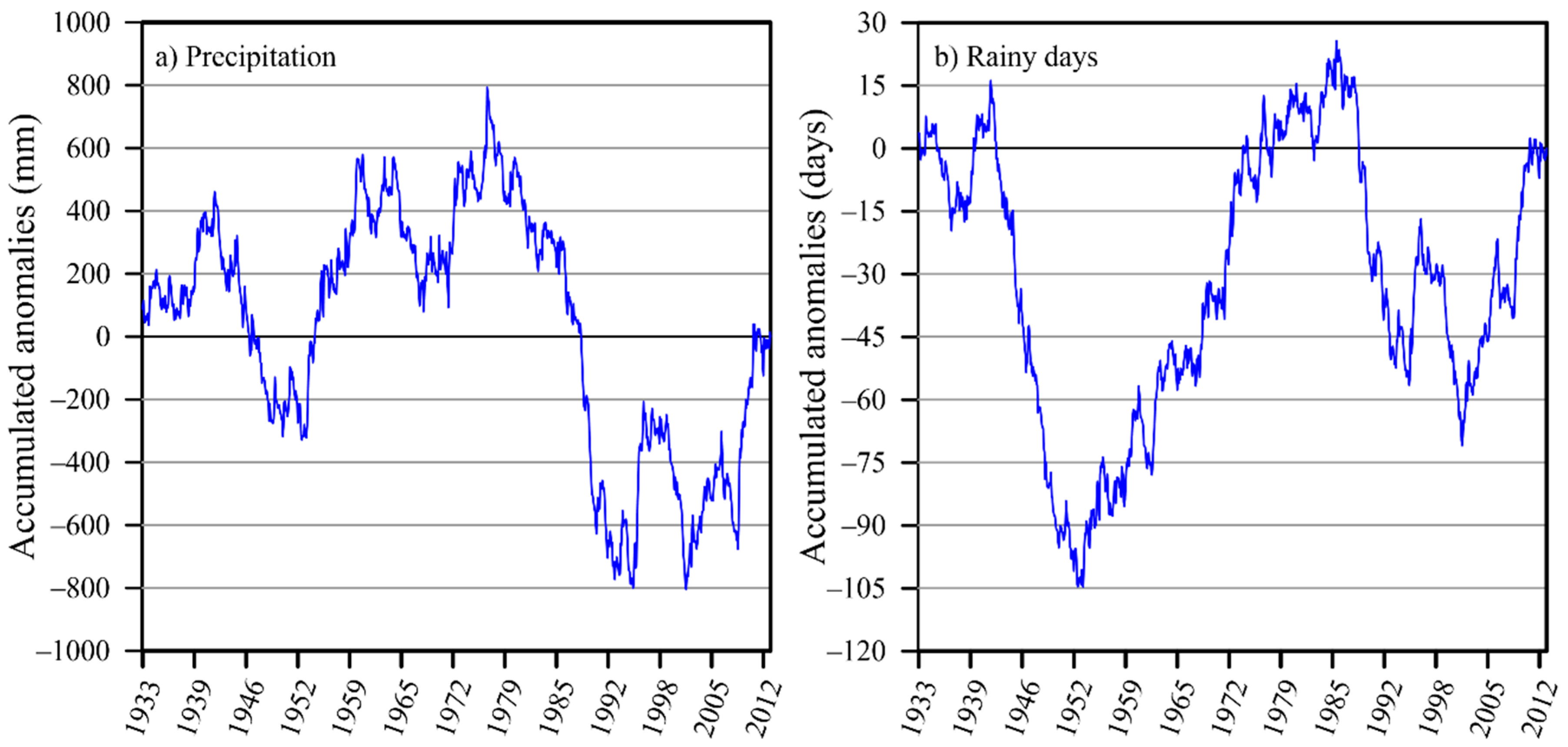
The accumulated anomalies were evaluated at each gauging station and for the whole Salento area (regional scale) using the historical monthly precipitation data, the number of rainy days and the monthly minimum, maximum and mean temperature records. For the sake of brevity, Figure 2 shows only the accumulated monthly precipitation anomalies and the ones relative to the number of rainy days over the Salento area. Periods with precipitation above and below the mean of the analyzed time interval (1933–2012) alternate until the second half of the 70s (Figure 2a), probably related to the natural fluctuation of the hydrological cycle. Then, a persistent downward slope of the accumulated anomalies indicates rainfall values lower than the mean until the mid-90s, when new fluctuations restart. According to Figure 2b, the number of rainy days shows an abrupt change point around the mid-50s, with a downward trend of the accumulated anomalies before 1950 (number of rainy days below the mean) followed by a period of rainy days above the mean (positive slope of the accumulated anomalies) until the mid-80s; fluctuations of different extent follow.
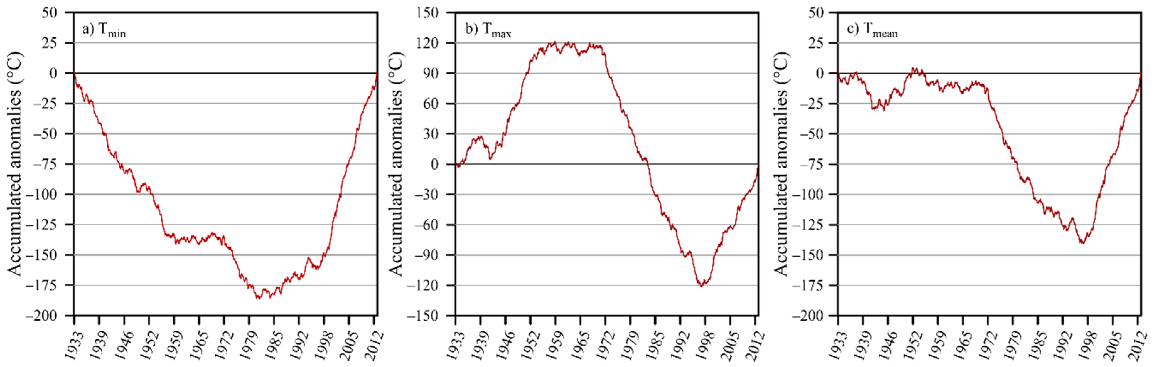
In Figure 3 the monthly accumulated anomalies of the minimum, maximum and mean temperature records at regional scale are shown. The accumulated anomalies of the minimum temperature data (Figure 3a) indicate a clear changing point around the 80s. A moderate downward slope (monthly temperature below the mean value) is detected until 1980 with a plateau (monthly temperature around the mean value) between 1960 and 1970. After 1980, the temperature is on average above its mean value (upward trend) with an increase in the slope of the accumulated anomalies (higher positive deviations from the mean) after 2000. The accumulated anomalies of the maximum temperature records have a different behavior (Figure 3b); after a period with values above the mean (with some fluctuations), a plateau between the mid-50 and 1970 is detected. Then the temperature stays below the mean and a changing point is detected at the end of the 90s when an upward trend starts. The monthly accumulated anomalies of the mean temperature data (Figure 3c) show moderate fluctuations around the mean until 1970, then a downward slope is detected (mean temperature below its mean) and a clear changing point is located at the end of the 90s followed by a period of temperature well above the mean (upward trend, higher slope).
Since changing points, plateaus and variations in the slope of the accumulated anomalies were detected for the climate variables, we chose to perform the further analyses (trend identification and quantification) not only for the whole period 1933–2012, but also for the shorter period 1976–2012 (in agreement also with Lionello et al. [20]).
3.2. Historical Trends
The trend analysis on the historical data was performed by means of the Mann-Kendall (MK) test and the Theil-Sen (TS) estimator. As mentioned before, two time intervals were chosen: the whole available period, 1933–2012, and the shorter one, 1976–2012. The analyses were conducted at each meteorological station and for the whole Salento area (regional scale) and at monthly and annual scale.
Figure 4 shows the monthly and annual precipitation trend gradients for the two periods as evaluated by the TS estimator; the box-whisker plots represent the variability between the 30 rain gauges; the solid line depicts the trend gradient at the regional scale with an indication of its significance (95% confidence level). Table 2 reports the results of the trend analyses at regional scale for both the precipitation and the rainy days at monthly and annual scale.
The trends, in the period 1933–2012, do not show considerable variations of the precipitation values (Figure 4a, Table 2), with alternating positive and negative gradients between months and stations; the tendencies are rarely significant (Table 2 for the Salento area; the MK test results for all the gauges are not shown for brevity). At regional scale, the analyses indicate a decreasing rainfall trend from October to February with a maximum negative gradient in December of about 3.3 mm/decade. March and April precipitation exhibits an increasing trend together with the September one, which presents a positive gradient of 2.5 mm/decade and a statistically significant tendency. From May to August the trend is almost absent, with a small positive rate in June and July and a negative gradient in May and August. The trend in the total annual precipitation is moderate and not statistically significant with a gradient of −2.4 mm/decade (compare with the value of −14.9 mm/decade of Lionello et al. [20] for the whole Apulia in the period 1951–2005).
In the shorter period 1976–2012 (Figure 4b) the precipitation trends, according to the regional time-series, are positive for all months but February, August and October; the tendencies are never statistically significant with the exception of September, which in addition presents the highest gradient (12.6 mm/decade in Table 2). The inter-station variability of the trend gradients is higher than that evaluated for the whole period. At annual scale, the trend of the total precipitation is positive with a gradient of about 41.1 mm/decade and the tendency is statistically significant.
No remarkable trends were identified for the monthly and annual number of rainy days over the Salento area (Table 2); the tendencies are always not significant with the exception of September, which exhibits a positive gradient of 0.25 rainy days/decade and 0.77 rainy days/decade for the periods 1933–2012 and 1976–2012, respectively.
The analysis of the historical temperature trends indicates a gradual warming of the Salento area. In the whole investigated period (1933–2012), the minimum temperature presents, according to the regional time-series, a positive trend for all months (Figure 5a, Table 3); the tendencies are always statistically significant with the exception of February, November and December. The highest positive gradients are found in the warm season with a maximum in May (0.30 °C/decade); the average annual minimum temperature increment is equal to 0.18 °C/decade (Table 3). Positive trend gradients are evaluated for all the analyzed temperature gauges with few exceptions at both monthly and annual scale (Figure 5a). In the period 1976–2012, according to the regional time-series, the minimum temperature exhibits a positive trend in all months but February (Figure 5b, Table 3). The trend gradients in the warm season are about three times higher than those estimated in the period 1933–2012, with a maximum rate in July and August of 0.79 °C/decade; the tendencies are statistically significant from April to September. At annual scale, the Salento area minimum temperature is increasing at a rate of 0.41 °C/decade and the trend is statistically significant.
The maximum temperature, according to the regional time-series in the period 1933–2012, shows small variations (Figure 5c) and the monthly trends are not statistically significant with the exception of January (0.09 °C/decade), July (−0.09 °C/decade) and September (−0.17 °C/decade). Whereas, in the period 1976–2012 (Figure 5d), the monthly trends are always positive and statistically significant for 8 months (Table 3, the exceptions are January, February, March and October). The highest gradients are in summer with a maximum in August equal to 1.09 °C/decade; the average annual maximum temperature increases at a rate of 0.57 °C/decade and the tendency is statistically significant. The maximum temperature gradients are positive for all stations, with very few exceptions (Figure 5d); however, the gradient spatial heterogeneity increases with respect to the period 1933–2012.
The mean temperature analysis shows, over the Salento area in the period 1933–2012, moderate positive trend gradients for all months but September (Figure 5e, Table 3). The only statistically significant trends, at the regional scale, are identified in January and May; the last month has also the highest gradient (0.17 °C/decade). The annual trend is statistically significant and indicates that the Salento area is warming at a rate of 0.07 °C/decade (Table 3, mean temperature). In the shorter period (1976–2012), the trends, according to the regional time-series, are positive in all months (Figure 5f, Table 3); the highest gradients are observed in summer with the maximum in August (0.97 °C/decade). The tendencies are statistically significant for the months from April to September and November and for the annual time-series, which points out that the mean temperature over the study area is increasing at a rate of 0.49 °C/decade (Table 3, mean temperature); all the stations show positive trend gradients with few exceptions (Figure 5f).
These results are comparable with the findings of Lionello et al. [20] for the whole Apulia, proving that the entire region is experiencing a warming trend that has mainly affected the late spring-summer seasons.
3.3. Regional Model Projections
To investigate the future climate over the Salento area, we made use of the data of 13 Regional Climate Models (RCMs, see Section 2). The monthly data were bias corrected, with reference to the whole Salento area (regional scale), according to the observations recorded in the period 1976–2005 (control period). The climate variables were then evaluated for three future periods, 2016–2035 (short term, ST), 2046–2065 (medium term, MT) and 2081–2100 (long term, LT), and a reference period (1986–2005, RP) for comparison. In the following, we report the analyses carried out on the monthly and annual precipitation and the monthly and annual mean temperature, under the two emission scenarios RCP4.5 and RCP8.5; all the results refer to the bias-corrected RCM data.
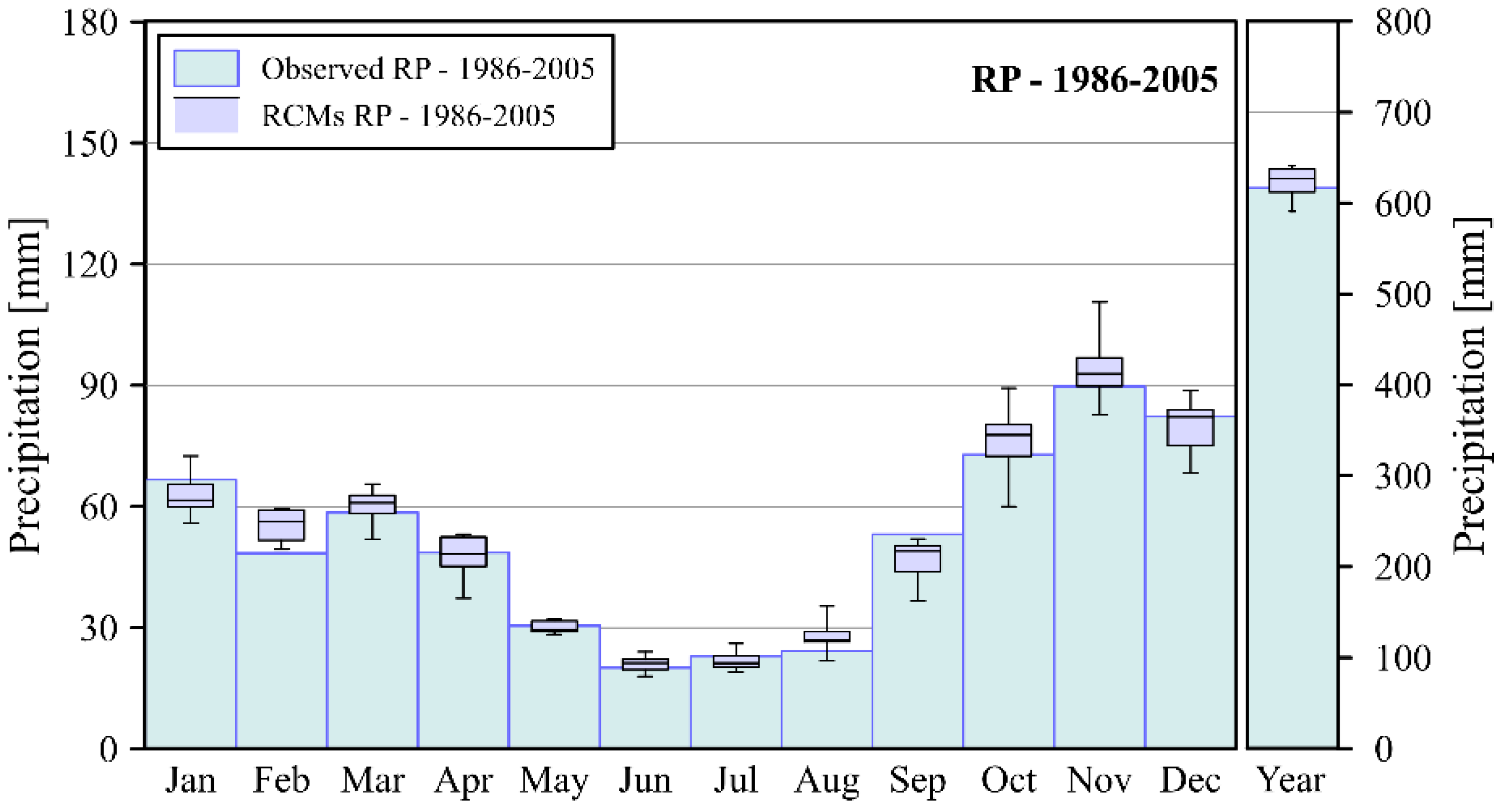
With reference to the annual total precipitation, according to the RCM ensemble mean, the climate models mimic very well the observed data in the reference period (Table 4, RP), with a deviation of about 1.2%; the interquartile range (IQR) of the RCM ensemble is 25.2 mm (Figure 6, the RCM variability is summarized with the box-whisker plots). At monthly scale, the precipitation regime is overall reproduced (Figure 6, Table 4, RP), although absolute deviations up to about 15% (ensemble mean) are identified in some months. In particular, in February, all the RCMs overestimate the observed precipitation (Figure 6) with a variation of 15% according to the ensemble mean (Table 4, RP); the deviation between the climate model ensemble mean and the observed value rises to 15.5% in August. In September, all the RCMs underestimate the observed precipitation with a deviation of 12.3% (Table 4, RP) according to the ensemble mean; in the other months the differences do not exceed 5.2%. It is noteworthy that, according to the observed precipitation, the deviations between each year value and the corresponding average in the control period (1976–2005) reach 66% at annual scale and exceed 400% at monthly scale; the RCM errors in reproducing the observed climate in the reference period (1986–2005) can therefore be ascribed to these very high interannual natural variations. The IQRs at monthly scale are between 2.5 mm and 8.8 mm denoting a very moderate inter-model variability in the reference period.
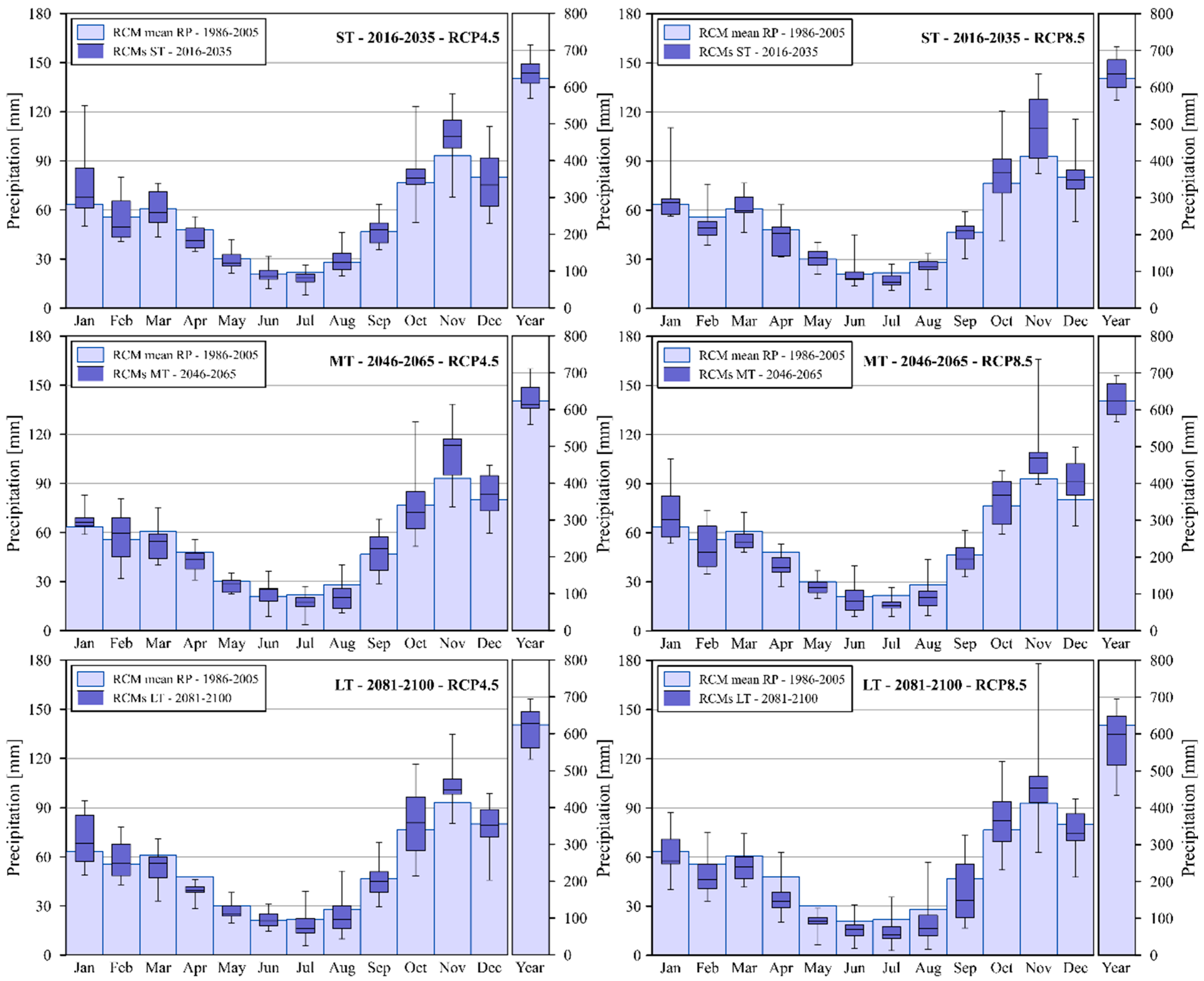
Figure 7 shows the precipitation projections for the three analyzed future periods and the two scenarios at monthly and annual scale. In each plot of Figure 7, the variability between the 13 RCMs is summarized with the box-whisker plots; the ensemble mean evaluated in the reference period (1986–2005) is depicted for comparison. Table 4 reports the RCM ensemble mean for the three future periods and the two RCPs at annual and monthly scale, together with the percentage variations with respect to the corresponding ensemble mean in the reference period. The robustness of the variations is also reported in Table 4; a variation is considered robust if at least 9 models of the 13 (more than 66%, [28]) agree in the direction of the change based on the RCM ensemble mean.
According to the RCP4.5 and the RCM ensemble mean (Table 4), the analysis does not detect significant changes in the annual precipitation between the three future periods and the reference one, with variations in the range +2.3% (ST) and −1.0% (LT); the changes are never robust. The variability among the RCMs is high with interquartile ranges (IQRs) of the annual precipitation of about 53 mm at ST, 55 mm at MT and 98 mm at LT; the IQRs result higher than the mean variations between the periods. At the short term, under the RCP4.5 scenario and according to the ensemble mean, the highest increases of the monthly precipitations, with respect to the reference period, are in January (+19.0%), November (+10.8%, robust change) and October (+6.9%), while the highest decreases are in April (−11.0%) and July (−16.5%) and they are both robust; the variations are below 5% in the other months. At the medium term (RCP4.5), the results (ensemble mean) indicate an increase in precipitation in the months from September to February and in June, the maximum is in November (+16.9%, robust change); in the other months, the precipitation decreases with a minimum in August (−24.3%) and a robust change of −21.6% in July. At the long term (RCP4.5), the highest decreases in precipitation (ensemble mean) are estimated from March to May and July (robust change) and August, with the maximum in April (−18.7%, robust change); the highest increments are in January (+9.3%) and November (+10.8%, robust change), while the variations are below 5% in the other months.
According to the RCP8.5 and the RCM ensemble mean (Table 4), the annual precipitation variations at short- and medium-term (with respect to the RP) are similar to the one estimated for the RCP4.5: +2.4% (IQR = 76 mm) at ST and +0.5% (IQR = 85 mm) at MT; the results indicate a decrease of 7.6% (IQR = 134 mm) at long-term; the changes are never robust. Also in this case, the IQRs result higher than the mean variations between the periods. At the short-term, positive and negative variations (ensemble mean) alternate between months, with the maximum increments in November (+20.2%, robust change) and the highest decreases in July (−22.0%, robust change) and August (−10.1%). At the medium-term, a decrease in precipitation (ensemble mean) is estimated from February to September with the maximum changes (robust) still in July (−24.0%) and August (−23.3%); the highest increase is in November of 18.2% (robust change). At the long-term, a decrease in precipitation is expected for all months but October (+6.3%) and November (+14.1%, robust change). The reduction in rainfall is higher than 24% from April to August with the maximum in July (−34.1%); the changes are robust in all cases.
The absolute variations in the annual rainfall between the three analyzed future periods and the reference one are in the range of about −50 mm and +15 mm; these values are comparable with the findings of Desiato et al. [17], although their signs are not always concordant in the same period. At monthly scale, the slight decrease of the precipitation in the summer season and a corresponding increase in the winter months, are in accordance with the study of Kapur et al. [19].
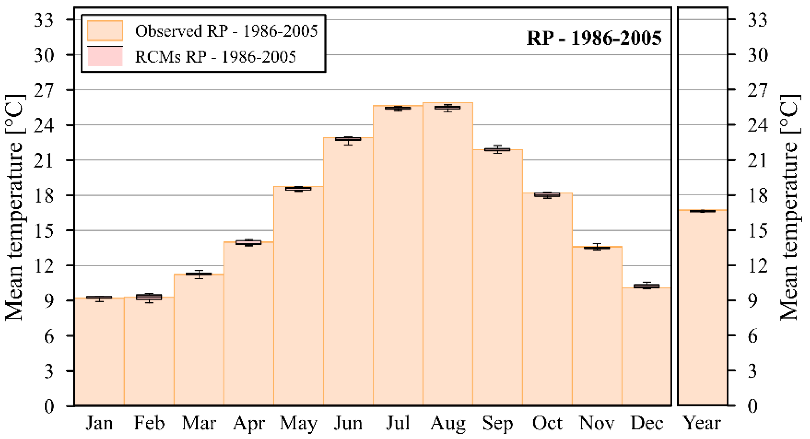
Figure 8 shows the comparison between the mean temperature observed and estimated by the RCMs (their variability is displayed with the box-whisker plots) in the reference period at monthly and annual scale. Thanks to the bias correction of the RCM data, the thermometric regime of the Salento area is accurately reproduced; according to the ensemble mean, the difference between the RCM annual mean temperature and the observed one, in the reference period, is equal to −0.1 °C (Table 5, RP); the RCM interquartile range (IQR) is 0.1 °C. At monthly scale, the maximum deviation is in August where the climate models (ensemble mean) underestimate the observed temperature of 0.4 °C; the inter-model variability (Figure 8) is moderate with IQRs between 0.1 °C and 0.4 °C.
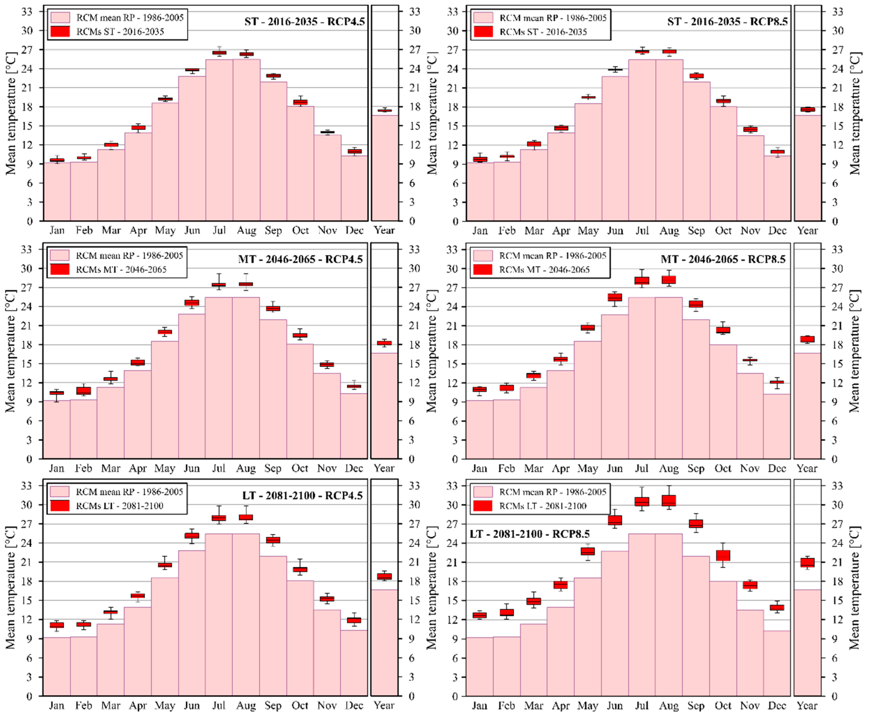
Figure 9 shows the temperature projections for the three future periods and the two RCPs at monthly and annual scale; the RCM variability is summarized with the box-whisker plots; the ensemble mean evaluated in the reference period (1986–2005) is depicted for comparison. Table 5 reports the RCM ensemble mean for the three future periods and the two RCPs at annual and monthly scale; the differences with respect to the corresponding ensemble mean in the reference period (and the robustness of the variations) are also presented to facilitate the result interpretation.
A progressive increase of the temperature over the Salento area is unequivocal according to all the RCMs projections and both the analyzed emission scenarios (Table 5, Figure 9); the changes are robust in all cases. At the short term, the RCMs (ensemble mean) estimate an increase of the mean temperature in all the months with respect to the reference period (Table 5); the IQRs of the RCM ensembles are in the range 0.2 ÷ 0.7 °C. The highest increases are found in the summer season, with a maximum in July of 1.16 °C (IQR = 0.5 °C) and 1.34 °C (IQR = 0.5 °C) under the RCP4.5 and RCP8.5, respectively. At annual scale, the temperature increases of 0.76 °C (IQR = 0.2 °C) for the RCP4.5 and 0.94 °C (IQR = 0.5 °C) for the RCP 8.5.
At the medium term, the temperature increases together with the uncertainty (variability between models); the IQRs of the climate model projections are now between 0.3 °C and 1.2 °C (monthly values). The highest increases in temperature are estimated in August, with differences with respect to the RP of 2.13 °C (IQR = 0.5 °C), for the RCP4.5, and 2.77 °C (IQR = 1.1 °C), for the RCP8.5. The annual temperature increases by 1.54 °C (IQR = 0.6 °C) under the RCP4.5 scenario, and 2.15 °C (IQR = 0.9 °C) for the RCP8.5.
At the long term, the annual temperature might be 2.06 °C (IQR = 0.9 °C) higher than the RP one (RCM ensemble mean) under the RCP4.5 and 4.17 °C (IQR = 1.4 °C) for the RCP8.5. At both the monthly and annual scale, the variability between the RCMs is higher than the previous period ones, with climate model IQRs in the range 0.4 ÷ 1.6 °C. The maximum increases are found in July and August (about 2.6 °C, IQR = 0.8 ÷ 0.9 °C) under the RCP4.5 scenario and about 5.2 °C (IQR = 1.3 ÷ 1.6 °C) under the RCP 8.5 scenario.
Overall, the outcomes of our study are in the range of the findings of Desiato et al. [17] for the whole Italy. The results of Kapur et al. [19], that show an increase in temperature of about 2 °C at the end of the century, are in agreement with our outcomes under the RCP4.5 scenario, while the estimation of Lionello et al. [20], an increase of 2 °C at 2050, better agree with our RCP8.5 results. As highlighted by these differences, it is important, besides the use of a large ensemble of climate models that helps in exploring their uncertainty, to make future projections according to different scenarios. The future rates of the greenhouse gas emissions are still unclear and conditioned by many factors that, although the political efforts toward their reduction worldwide, suggest to explore multiple working hypothesis, as in the old concept of Chamberlin [32].
3.4. Future Heat Waves
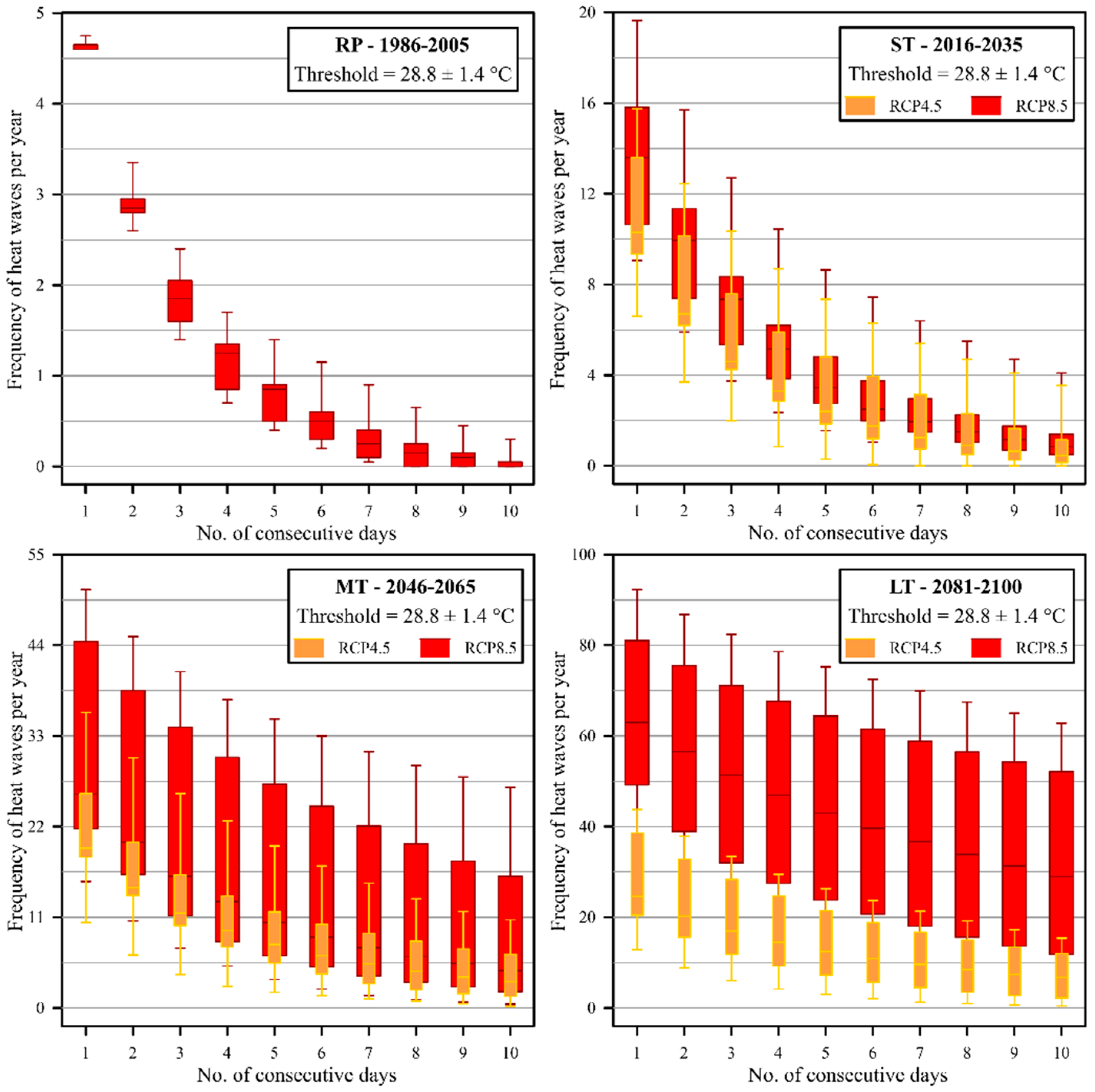
We used the daily temperature data of the 13 Regional Climate Models (RCMs) to identify potential future changes in the characteristics of the heat waves. We say that a heat wave occurs when the daily mean temperature exceeds a chosen threshold for at least a selected number of consecutive days. In this work, the threshold is model dependent and for each RCM corresponds to the 95th percentile of the June, July and August daily mean temperature projections in the reference period (1986–2005). The threshold is equal to 28.8 ± 1.4 °C, where the variability corresponds to the 95% confidence interval (based on the ensemble of the 13 thresholds).
Figure 10 shows the frequency of the heat waves per year (number of threshold exceedances per year) for different values of consecutive days for the reference period (RP) and at the short-, medium-, and long-term, for both the RCP4.5 and the RCP8.5; the variability between the climate models is summarized by means of the box-whisker plots. Table 6 sums up the results reporting the frequency of the heat waves per year in terms of RCM ensemble mean. The heat waves progressively increase over time; the threshold exceedances are higher for the RCP8.5 than the RCP4.5. With reference to 5 consecutive days and the ensemble mean, the number of exceedances is about 1 per year in the reference period, about 3 at ST, 10 at MT and 13 at LT according to the RCP4.5; the values increase to 4 at ST, 17 at MT and 45 at LT for the RCP8.5.
The uncertainty is high and the inter-model variability increases in time; however, the mean results are alarming. This aspect should not be overlooked, especially in an area like the Salento where the summer season is already hot and dry. The social and economic impacts of more frequent heat waves could be significant, since the population health, the biodiversity and the ecosystems, as well as tourism and the crop yields, are directly affected. In this context, the study of Ahmadalipour et al. [16] shows that the morbidity and mortality risk, for people aged over 65 years, due to excessive heat stress is expected to increase in the Middle East and North Africa region (that encompasses the Salento area) for the 21st century; the population should be more aware of the importance of these problems. In addition, the high mortality risk, related to the intensification of the extreme temperature and heatwaves emphasizes the necessity of climate change mitigation and adaptation strategies.
4. Conclusions
In this study, historical monthly precipitation and temperature data recorded in the Salento area in the period 1933–2012 were analyzed to identify changing points and trends in the time-series. The accumulated anomalies of the minimum and maximum temperature showed a clear changing point around the 80s and at the end of the 90s, respectively. A positive trend of the minimum temperature, statistically significant for almost all months, is detected in the period 1933–2012 with the highest gradients in the warm season; the trend gradients considerably increase in the shorter period 1976–2012. At annual scale, the Salento area minimum temperature has increased at a rate of 0.18 and 0.41 °C/decade in the period 1933–2012 and 1976–2012, respectively. The maximum temperature does not show significant variations in the period 1933–2012 but the monthly trends are always positive and often statistically significant in the period 1976–2012, with a higher gradient in summer and an annual increasing rate of 0.57 °C/decade. The monthly precipitation trends, in the period 1933–2012, are not significant with the exception of September that presents an increasing gradient of 2.5 mm/decade; the total annual precipitation has decreased at a rate of 2.4 mm/decade. In the period 1976–2012 the Salento precipitation trends are positive for many months although they are not statistically significant with the exception of September (+12.6 mm/decade, compare with 53.6 mm, the mean September rainfall in the period 1986–2005); the trend of the total precipitation is positive (+41.1 mm/decade) and statistically significant. Also the number of September rainy days presents a positive and significant trend in both the analyzed periods; a tendency that could affect the beach tourism, which is generally still high in this month.
We then used 13 GCM-RCM climate projections of the EURO-CORDEX ensemble, under the RCP4.5 and RCP8.5 scenarios, to assess the future climate over the Salento area at short—(2016–2035), medium—(2046–2065) and long-term (2081–2100). According to the RCM ensemble mean, no significant (−1.0 ÷ +2.3% with the exception of the RCP8.5 at long-term, that is −7.6%) and robust variations (with respect to the reference period 1986–2005) are expected for the future total annual rainfall. However, the inter-model variability, the period being equal, often exceeds the expected future changes. Systematic changes are present in some months; in particular, robust decreases of the April (−8.0 ÷ −24.5%) and July (−15.0 ÷ −34.1%) precipitation are estimated for three analyzed periods and both the RCP scenarios, as well as robust increases in November (+10.8 ÷ 20.2%).
The gradual increase of the Salento temperature, already detectable through the analysis of the historical data, is confirmed by the climate model projections. All the analyzed models agree (robust change) on the increasing of the mean temperature over the century for all months with the highest positive variations in the warm season (May–September). The annual mean temperature could be more than 2 °C higher (with respect to the 1986–2005 one) at the end of this century according to the RCP4.5 scenario and reaches an increment of about 4 °C under the RCP8.5.
In addition to the above analyses that makes use of monthly data, we took advantage of the daily temperature projections of the climate models to identify potential variations in the characteristics of the heat waves. Despite the high inter-model variability, the frequency of the heat waves per year is expected to gradually increase over the century.
Increasing temperature and decreasing rainfall can also negatively impact water resources, both in terms of quantity and quality [33], in an area that already has a water budget deficit, imports water from the neighboring regions [20] and overexploits its coastal aquifers with increasing salinization problems [34]. Our work can be a starting point but further studies are required to investigate these not so obvious and local aspects.
Finally, we believe that local studies are also important to raise awareness about climate change consequences in the population and the regional authorities and can help to promote feasible development policies and sustainable mitigation plans, which are essential to reach the global goal set during the COP21.
Author Contributions
All the authors contributed equally in conceiving, developing and writing the article.
Funding
This research received no external funding.
Conflicts of Interest
The authors declare no conflict of interest.
References
- Intergovernmental Panel on Climate Change (IPCC). Climate Change 2014: Synthesis Report. Contribution of Working Groups I, II and III to the Fifth Assessment Report of the Intergovernmental Panel on Climate Change; Core Writing Team, Pachauri, R.K., Meyer, L.A., Eds.; IPCC: Geneva, Switzerland, 2014. [Google Scholar]
- United Nations Framework Convention on Climate Change (UNFCCC). Paris Agreement. 2015. Available online: https://unfccc.int/process/conferences/pastconferences/paris-climate-change-conference-november-2015/paris-agreement (accessed on 27 June 2018).
- Giorgi, F. Climate change hot-spots. Geophys. Res. Lett. 2006, 33, L08707. [Google Scholar] [CrossRef]
- Philandras, C.M.; Nastos, P.T.; Kapsomenakis, J.; Douvis, K.C.; Tselioudis, G.; Zerefos, C.S. Long term precipitation trends and variability within the Mediterranean region. Nat. Hazards Earth Syst. Sci. 2011, 11, 3235–3250. [Google Scholar] [CrossRef] [Green Version]
- Desiato, F.; Fioravanti, G.; Fraschetti, P.; Perconti, W.; Piervitali, E.; Pavan, V. Gli Indicatori del CLIMA in Italia nel 2016. (Climate Indicators in Italy 2016); Stato dell’Ambiente; The Italian National Institute for Environmental Protection and Research (ISPRA): Rome, Italy, 2017; Volume 72, ISBN 978-88-448-0723-8. (In Italian) [Google Scholar]
- Turco, M.; Llasat, M.C.; Herrera, S.; Gutiérrez, J.M. Bias correction and downscaling of future RCM precipitation projections using a MOS-Analog technique. J. Geophys. Res. Atmos. 2017, 122, 2631–2648. [Google Scholar] [CrossRef] [Green Version]
- Hostetler, S.W.; Alder, J.R.; Allan, A.M. Dynamically Downscaled Climate Simulations over North America: Methods, Evaluation, and Supporting Documentation for Users; Open-File Report 2011-1238; U.S. Geological Survey: Reston, VA, USA, 2011; p. 64.
- Christensen, J.H.; Boberg, F.; Christensen, O.B.; Lucas-Picher, P. On the need for bias correction of regional climate change projections of temperature and precipitation. Geophys. Res. Lett. 2008, 35, L20709. [Google Scholar] [CrossRef]
- Teutschbein, C.; Seibert, J. Bias correction of regional climate model simulations for hydrological climate-change impact studies: Review and evaluation of different methods. J. Hydrol. 2012, 456–457, 12–29. [Google Scholar] [CrossRef]
- D’Oria, M.; Ferraresi, M.; Tanda, M.G. Historical trends and high-resolution future climate projections in northern Tuscany (Italy). J. Hydrol. 2017, 555, 708–723. [Google Scholar] [CrossRef]
- Alpert, P.; Krichak, S.O.; Shafir, H.; Haim, D.; Osetinsky, I. Climatic trends to extremes employing regional modeling and statistical interpretation over the E. Mediterranean. Glob. Planet. Chang. 2008, 63, 163–170. [Google Scholar] [CrossRef]
- Giorgi, F.; Lionello, P. Climate change projections for the Mediterranean region. Glob. Planet. Chang. 2008, 63, 90–104. [Google Scholar] [CrossRef]
- Dubrovský, M.; Hayes, M.; Duce, P.; Trnka, M.; Svoboda, M.; Zara, P. Multi-GCM projections of future drought and climate variability indicators for the Mediterranean region. Reg. Environ. Chang. 2014, 14, 1907–1919. [Google Scholar] [CrossRef]
- Ozturk, T.; Ceber, Z.P.; Türkeş, M.; Kurnaz, M.L. Projections of climate change in the Mediterranean Basin by using downscaled global climate model outputs. Int. J. Climatol. 2015, 35, 4276–4292. [Google Scholar] [CrossRef]
- Zittis, G.; Hadjinicolaou, P.; Fnais, M.; Lelieveld, J. Projected changes in heat wave characteristics in the eastern Mediterranean and the Middle East. Reg. Environ. Chang. 2016, 16, 1863–1876. [Google Scholar] [CrossRef]
- Ahmadalipour, A.; Moradkhani, H. Escalating heat-stress mortality risk due to global warming in the Middle East and North Africa (MENA). Environ. Int. 2018, 117, 215–225. [Google Scholar] [CrossRef] [PubMed]
- Desiato, F.; Fioravanti, G.; Fraschetti, P.; Perconti, W.; Piervitali, E. Il Clima Futuro in Italia: Analisi delle Proiezioni dei Modelli Regionali (The Future Climate in Italy: Analysis of the Regional Model Projections); Stato dell’Ambiente; The Italian National Institute for Environmental Protection and Research (ISPRA): Rome, Italy, 2015; Volume 58, ISBN 978-88-448-0723-8. (In Italian) [Google Scholar]
- Ruti, P.M.; Somot, S.; Giorgi, F.; Dubois, C.; Flaounas, E.; Obermann, A.; Dell’Aquilla, A.; Pisacane, G.; Harzallah, A.; Lombardi, E.; et al. MED-CORDEX initiative for Mediterranean Climate studies. Bull. Am. Meteorol. Soc. 2016, 97, 1187–1208. [Google Scholar] [CrossRef]
- Kapur, B.; Steduto, P.; Todorovic, M. Prediction of Climatic Change for the Next 100 Years in the Apulia Region, Southern Italy. Ital. J. Agron. 2007, 2, 365–372. [Google Scholar] [CrossRef]
- Lionello, P.; Congedi, L.; Reale, M.; Scarascia, L.; Tanzarella, A. Sensitivity of typical Mediterranean crops to past and future evolution of seasonal temperature and precipitation in Apulia. Reg. Environ. Chang. 2013, 14, 2025–2038. [Google Scholar] [CrossRef]
- Mann, H.B. Non parametric tests against trend. Econometrica 1945, 13, 245–259. [Google Scholar] [CrossRef]
- Kendall, M.G. Rank Correlation Methods, 4th ed.; Griffin: London, UK, 1975. [Google Scholar]
- Sen, P.K. Estimates of the regression coefficient based on Kendall’s tau. J. Am. Stat. Assoc. 1968, 63, 1379–1389. [Google Scholar] [CrossRef]
- Van der Linden, P.; Mitchell, J.F.B. ENSEMBLES: Climate Change and Its Impacts: Summary of Research and Results from the ENSEMBLES Project; Met Office Hadley Centre: Exeter, UK, 2009.
- Gualdi, S.; Somot, S.; May, W.; Castellari, S.; Déqué, M.; Adani, M.; Artale, V.; Bellucci, A.; Breitgand, J.S.; Carillo, A.; et al. Future Climate Projections. In Regional Assessment of Climate Change in the Mediterranean; Navarra, A., Tubiana, L., Eds.; Springer: Dordrecht, The Netherlands, 2013; ISBN 978-94-007-5781-3. [Google Scholar]
- Nakicenovic, N.; Alcamo, J.; Davis, G.; De Vries, B.; Fenhann, J.; Gaffin, S.; Gregory, K.; Grübler, A.; Jung, T.Y.; Kram, T.; et al. IPCC Special Report on Emission Scenarios; Cambridge University Press: Cambridge, UK, 2000. [Google Scholar]
- Intergovernmental Panel on Climate Change (IPCC). Climate Change 2007: Synthesis Report. Contribution of Working Groups I, II and III to the Fourth Assessment Report of the Intergovernmental Panel on Climate Change; Core Writing Team, Pachauri, R.K., Reisinger, A., Eds.; IPCC: Geneva, Switzerland, 2007. [Google Scholar]
- Jacob, D.; Petersen, J.; Eggert, B.; Alias, A.; Christensen, O.B.; Bouwer, L.M.; Braun, A.; Colette, A.; Déqué, M.; Georgievski, G.; et al. EURO-CORDEX: New high-resolution climate change projections for European impact research. Reg. Environ. Chang. 2014, 14, 563–578. [Google Scholar] [CrossRef]
- Allen, R.G.; Pereira, L.S.; Raes, D.; Smith, M. Crop Evapotranspiration: Guidelines for Computing Crop Water Requirements; FAO Irrigation and Drainage Paper 56; FAO: Rome, Italy, 1998; ISBN 92-5-104219-5. [Google Scholar]
- Lozowski, E.P.; Charlton, R.B.; Nguyen, C.D.; Wilson, J.D. The Use of Cumulative Monthly Mean Temperature Anomalies in the Analysis of Local Interannual Climate Variability. J. Clim. 1989, 2, 1059–1068. [Google Scholar] [CrossRef] [Green Version]
- Hamed, K.H.; Rao, A.R. A modified Mann-Kendall trend test for autocorrelated data. J. Hydrol. 1998, 204, 182–196. [Google Scholar] [CrossRef]
- Chamberlin, T.C. The method of multiple working hypotheses. Science 1890, 15, 92–96. [Google Scholar] [CrossRef]
- Delle Rose, M.; Martano, P. Infiltration and Short-Time Recharge in Deep Karst Aquifer of the Salento Peninsula (Southern Italy): An Observational Study. Water 2018, 10, 260. [Google Scholar] [CrossRef]
- Parisi, A.; Monno, V.; Fidelibus, M.D. Cascading vulnerability scenarios in the management of groundwater depletion and salinization in semi-arid areas. Int. J. Disaster Risk Reduct. 2018. [Google Scholar] [CrossRef]
Figure 1.
Study area, temperature and rain gauging station locations and portion of the EUR-11 RCM grid. Overlapping symbols identify temperature and rain gauges located in the same position.
Figure 1.
Study area, temperature and rain gauging station locations and portion of the EUR-11 RCM grid. Overlapping symbols identify temperature and rain gauges located in the same position.

Figure 2.
Accumulated anomalies of the monthly precipitation records (a) and the number of rainy days (b) for the Salento area.
Figure 2.
Accumulated anomalies of the monthly precipitation records (a) and the number of rainy days (b) for the Salento area.

Figure 3.
Accumulated anomalies of the monthly minimum (Tmin, (a)), maximum (Tmax, (b)) and mean (Tmean, (c)) temperature records for the Salento area.
Figure 3.
Accumulated anomalies of the monthly minimum (Tmin, (a)), maximum (Tmax, (b)) and mean (Tmean, (c)) temperature records for the Salento area.

Figure 4.
Monthly and annual precipitation trend gradients as evaluated by the Theil-Sen estimator: (a) whole period 1933–2012; (b) shorter period 1976–2012. The box-whisker plots represent the variability between the 30 rain gauges (the whiskers indicate the minimum and maximum values); the solid line depicts the trend gradient for the whole Salento area with an indication of its significance (95% confidence level).

Figure 5.
Monthly and annual temperature trend gradients as evaluated by the Theil-Sen estimator: minimum temperature (Tmin, (a)), maximum temperature (Tmax, (c)) and mean temperature (Tmean, (e)) for the whole period 1933–2012; Tmin (b), Tmax (d), Tmean (f) for the shorter period 1976–2012. The box-whisker plots represent the variability between the 18 temperature gauges (the whiskers indicate the minimum and maximum values); the solid line depicts the trend gradient for the whole Salento area with an indication of its significance (95% confidence level).

Figure 6.
Monthly and annual precipitation over the Salento area, observed and evaluated by the RCMs in the reference period (RP). The box-whisker plots represent the variability between the 13 RCMs (the whiskers indicate the minimum and maximum values).
Figure 6.
Monthly and annual precipitation over the Salento area, observed and evaluated by the RCMs in the reference period (RP). The box-whisker plots represent the variability between the 13 RCMs (the whiskers indicate the minimum and maximum values).

Figure 7.
Monthly and annual precipitation, over the Salento area, evaluated by the RCMs at the short—(ST), medium—(MT) and long-term (LT) under the RCP4.5 and RCP8.5 scenarios. The box-whisker plots represent the variability between the 13 RCMs (the whiskers indicate the minimum and maximum values). Bars of the RCM ensemble mean in the reference period (RP).

Figure 8.
Monthly and annual mean temperature over the Salento area, observed and evaluated by the RCMs in the reference period (RP). The box-whisker plots represent the variability between the 13 RCMs (the whiskers indicate the minimum and maximum values).
Figure 8.
Monthly and annual mean temperature over the Salento area, observed and evaluated by the RCMs in the reference period (RP). The box-whisker plots represent the variability between the 13 RCMs (the whiskers indicate the minimum and maximum values).

Figure 9.
Monthly and annual mean temperature, over the Salento area, evaluated by the RCMs at the short—(ST), medium—(MT) and long-term (LT) under the RCP4.5 and RCP8.5 scenarios. The box-whisker plots represent the variability between the 13 RCMs (the whiskers indicate the minimum and maximum values). Bars of the RCM ensemble mean in the reference period (RP).

Figure 10.
Frequency of the heat waves per year for different values of consecutive days in the reference period (RP) and at the short—(ST), medium—(MT), and long-term (LT), as evaluated by the RCM projections under the RCP4.5 and RCP8.5 scenarios. The box-whisker plots represent the variability between the 13 RCMs (the whiskers indicate the minimum and maximum values). Pay attention to the different vertical scales.


Table 1.
EURO-CORDEX ensemble (www.euro-cordex.net), combination of different RCMs and GCMs, adopted in this study.
Table 1.
EURO-CORDEX ensemble (www.euro-cordex.net), combination of different RCMs and GCMs, adopted in this study.
| GCM | ||||||
|---|---|---|---|---|---|---|
| CNRM-CM5 | EC-EARTH | HadGEM2-ES | MPI-ESM-LR | IPSL-CM5A-MR | ||
| RCM | CCLM4-8-17 | X | X | X | X | |
| HIRHAM5 | X | |||||
| WRF331F | X | |||||
| RACMO22E | X | X | ||||
| RCA4 | X | X | X | X | X | |
Table 2.
Monthly and annual trend gradients, β as evaluated by the Theil-Sen estimator (precipitation, [mm/decade], number of rainy days [rainy days/decade]) and trend significance, at 95% confidence level, S (0, no trend, 1, trend exists) for the Salento area: whole period 1933–2012 and shorter period 1976–2012.
| Precipitation | No. of Rainy Days | |||||||
|---|---|---|---|---|---|---|---|---|
| 1933–2012 | 1976–2012 | 1933–2012 | 1976–2012 | |||||
| S | S | S | S | |||||
| January | −3.01 | 0 | 2.33 | 0 | −0.27 | 0 | 0.24 | 0 |
| February | −0.32 | 0 | −1.68 | 0 | 0.15 | 0 | −0.27 | 0 |
| March | 1.68 | 0 | 3.59 | 0 | 0.08 | 0 | −0.24 | 0 |
| April | 1.97 | 0 | 2.83 | 0 | 0.29 | 1 | 0.46 | 0 |
| May | −0.35 | 0 | 3.58 | 0 | −0.05 | 0 | 0.14 | 0 |
| June | 0.24 | 0 | 1.68 | 0 | 0.06 | 0 | 0.14 | 0 |
| July | 0.75 | 0 | 2.11 | 0 | 0.10 | 0 | 0.16 | 0 |
| August | −0.42 | 0 | −3.29 | 0 | −0.01 | 0 | −0.42 | 0 |
| September | 2.49 | 1 | 12.60 | 1 | 0.25 | 1 | 0.77 | 1 |
| October | −1.50 | 0 | −1.32 | 0 | −0.06 | 0 | 0.06 | 0 |
| November | −0.99 | 0 | 3.29 | 0 | 0.00 | 0 | −0.28 | 0 |
| December | −3.28 | 0 | 7.89 | 0 | 0.04 | 0 | 0.62 | 0 |
| Year | −2.39 | 0 | 41.06 | 1 | 0.61 | 0 | 0.91 | 0 |
Table 3.
Monthly and annual minimum temperature (Tmin), maximum temperature (Tmax) and mean temperature (Tmean) trend gradients as evaluated by the Theil-Sen estimator ( [°C/decade]) and trend significance, at 95% confidence level, S (0, no trend, 1, trend exists) for the Salento area: whole period 1933–2012 and shorter period 1976–2012.
| Tmin | Tmax | Tmean | ||||||||||
|---|---|---|---|---|---|---|---|---|---|---|---|---|
| 1933–2012 | 1976–2012 | 1933–2012 | 1976–2012 | 1933–2012 | 1976–2012 | |||||||
| S | S | S | S | S | S | |||||||
| January | 0.20 | 1 | 0.13 | 0 | 0.09 | 1 | 0.22 | 0 | 0.15 | 1 | 0.17 | 0 |
| February | 0.09 | 0 | −0.15 | 0 | −0.05 | 0 | 0.22 | 0 | 0.03 | 0 | 0.13 | 0 |
| March | 0.20 | 1 | 0.19 | 0 | 0.04 | 0 | 0.35 | 0 | 0.11 | 0 | 0.23 | 0 |
| April | 0.17 | 1 | 0.47 | 1 | −0.10 | 0 | 0.73 | 1 | 0.04 | 0 | 0.61 | 1 |
| May | 0.30 | 1 | 0.53 | 1 | 0.06 | 0 | 0.71 | 1 | 0.17 | 1 | 0.65 | 1 |
| June | 0.25 | 1 | 0.71 | 1 | −0.02 | 0 | 0.94 | 1 | 0.12 | 0 | 0.82 | 1 |
| July | 0.24 | 1 | 0.79 | 1 | −0.09 | 1 | 0.88 | 1 | 0.08 | 0 | 0.86 | 1 |
| August | 0.27 | 1 | 0.79 | 1 | −0.02 | 0 | 1.09 | 1 | 0.13 | 0 | 0.97 | 1 |
| September | 0.13 | 1 | 0.57 | 1 | −0.17 | 1 | 0.42 | 1 | −0.02 | 0 | 0.51 | 1 |
| October | 0.15 | 1 | 0.16 | 0 | −0.08 | 0 | 0.32 | 0 | 0.04 | 0 | 0.24 | 0 |
| November | 0.07 | 0 | 0.33 | 0 | −0.05 | 0 | 0.59 | 1 | 0.00 | 0 | 0.41 | 1 |
| December | 0.09 | 0 | 0.07 | 0 | 0.00 | 0 | 0.27 | 1 | 0.05 | 0 | 0.18 | 0 |
| Year | 0.18 | 1 | 0.41 | 1 | −0.05 | 0 | 0.57 | 1 | 0.07 | 1 | 0.49 | 1 |
Table 4.
Monthly and annual precipitation over the whole Salento area, for the reference period (RP, 1986−2005), at the short—(ST, 2016−2035), medium—(MT, 2046−2065) and long-term (LT, 2081−2100). Observed values (Obs., [mm]), RCM ensemble mean (, [mm]) under the RCP4.5 and RCP8.5 scenarios and percentage differences (Diff., [%]) between the projections at ST, MT, LT and the RP ones; the symbol * means that the change is robust.
| RCP4.5 | RCP8.5 | |||||||||||||
|---|---|---|---|---|---|---|---|---|---|---|---|---|---|---|
| RP | ST | MT | LT | ST | MT | LT | ||||||||
| Obs. | Diff. | Diff. | Diff. | Diff. | Diff. | Diff. | ||||||||
| J | 66.55 | 63.29 | 75.33 | +19.0 | 68.09 | +7.6 | 69.15 | +9.3 | 67.66 | +6.9 | 70.98 | +12.1 | 61.26 | −3.2 |
| F | 48.32 | 55.57 | 54.38 | −2.1 | 56.94 | +2.5 | 58.18 | +4.7 | 51.20 | −7.9 * | 50.75 | −8.7 | 49.09 | −11.7 * |
| M | 58.43 | 60.73 | 61.51 | +1.3 | 52.58 | −13.4 * | 53.93 | −11.2 * | 61.49 | +1.2 | 55.81 | −8.1 * | 55.71 | −8.3 * |
| A | 48.46 | 47.86 | 42.58 | −11.0 * | 43.13 | −9.9 * | 38.92 | −18.7 * | 44.05 | −8.0 * | 40.13 | −16.2 * | 36.15 | −24.5 * |
| M | 30.39 | 29.96 | 29.24 | −2.4 | 27.71 | −7.5 | 26.65 | −11.1 | 30.53 | +1.9 | 27.05 | −9.7 * | 20.22 | −32.5 * |
| J | 19.97 | 20.89 | 20.43 | −2.2 | 22.55 | +7.9 | 21.94 | +5.0 * | 21.82 | +4.4 | 19.76 | −5.4 | 15.87 | −24.0 * |
| J | 22.81 | 21.63 | 18.06 | −16.5 * | 16.97 | −21.6 * | 18.39 | −15.0 * | 16.87 | −22.0 * | 16.44 | −24.0 * | 14.26 | −34.1 * |
| A | 24.12 | 27.86 | 29.07 | +4.3 | 21.08 | −24.3 | 24.34 | −12.7 | 25.06 | −10.1 | 21.36 | −23.3 * | 21.10 | −24.3 * |
| S | 53.02 | 46.50 | 46.84 | +0.7 | 49.19 | +5.8 * | 44.83 | −3.6 | 46.31 | −0.4 | 45.08 | −3.1 | 40.35 | −13.2 |
| O | 72.74 | 76.42 | 81.72 | +6.9 | 77.15 | +1.0 | 79.95 | +4.6 | 81.88 | +7.2 * | 79.97 | +4.6 | 81.24 | +6.3 |
| N | 89.62 | 92.93 | 102.98 | +10.8 * | 108.63 | +16.9 * | 102.97 | +10.8 * | 111.71 | +20.2 * | 109.87 | +18.2 * | 106.03 | +14.1 * |
| D | 82.13 | 80.05 | 76.06 | −5.0 | 82.50 | +3.1 | 77.96 | −2.6 | 80.28 | +0.3 | 89.70 | +12.1 * | 75.26 | −6.0 |
| Y | 616.56 | 623.70 | 638.20 | +2.3 | 626.51 | +0.5 | 617.19 | −1.0 | 638.87 | +2.4 | 626.90 | +0.5 | 576.53 | −7.6 |
Table 5.
Monthly and annual mean temperature, over the whole Salento area, for the reference period (RP, 1986–2005), at the short—(ST, 2016–2035), medium—(MT, 2046–2065) and long-term (LT, 2081–2100). Observed values (Obs., [°C]), RCM ensemble mean (, [°C]) under the RCP4.5 and RCP8.5 scenarios and differences (Diff., [°C]) between the projections at ST, MT, LT and the RP ones; the symbol * means that the change is robust.
| RCP4.5 | RCP8.5 | |||||||||||||
|---|---|---|---|---|---|---|---|---|---|---|---|---|---|---|
| RP | ST | MT | LT | ST | MT | LT | ||||||||
| Obs. | Diff. | Diff. | Diff. | Diff. | Diff. | Diff. | ||||||||
| J | 9.18 | 9.19 | 9.58 | 0.39 * | 10.33 | 1.13 * | 10.98 | 1.79 * | 9.84 | 0.65 * | 10.93 | 1.74 * | 12.68 | 3.49 * |
| F | 9.27 | 9.27 | 9.98 | 0.71 * | 10.67 | 1.40 * | 11.10 | 1.83 * | 10.21 | 0.93 * | 11.13 | 1.85 * | 13.04 | 3.76 * |
| M | 11.21 | 11.24 | 11.98 | 0.74 * | 12.67 | 1.43 * | 13.08 | 1.84 * | 12.07 | 0.83 * | 13.16 | 1.92 * | 14.86 | 3.62 * |
| A | 13.97 | 13.91 | 14.57 | 0.67 * | 15.12 | 1.21 * | 15.60 | 1.69 * | 14.65 | 0.74 * | 15.76 | 1.85 * | 17.46 | 3.55 * |
| M | 18.72 | 18.54 | 19.24 | 0.70 * | 19.96 | 1.42 * | 20.62 | 2.08 * | 19.49 | 0.95 * | 20.59 | 2.05 * | 22.63 | 4.08 * |
| J | 22.89 | 22.74 | 23.73 | 1.00 * | 24.53 | 1.80 * | 25.05 | 2.31 * | 23.83 | 1.10 * | 25.29 | 2.55 * | 27.53 | 4.79 * |
| J | 25.63 | 25.39 | 26.55 | 1.16 * | 27.50 | 2.11 * | 27.96 | 2.57 * | 26.73 | 1.34 * | 28.11 | 2.72 * | 30.57 | 5.18 * |
| A | 25.89 | 25.44 | 26.32 | 0.87 * | 27.57 | 2.13 * | 28.03 | 2.59 * | 26.71 | 1.27 * | 28.22 | 2.77 * | 30.59 | 5.15 * |
| S | 21.88 | 21.89 | 22.88 | 0.98 * | 23.68 | 1.79 * | 24.40 | 2.50 * | 22.92 | 1.02 * | 24.24 | 2.35 * | 26.87 | 4.97 * |
| O | 18.17 | 18.02 | 18.73 | 0.72 * | 19.45 | 1.43 * | 20.02 | 2.00 * | 18.89 | 0.87 * | 20.24 | 2.23 * | 21.94 | 3.92 * |
| N | 13.57 | 13.49 | 13.95 | 0.46 * | 14.85 | 1.36 * | 15.27 | 1.78 * | 14.43 | 0.94 * | 15.58 | 2.09 * | 17.30 | 3.81 * |
| D | 10.08 | 10.23 | 10.93 | 0.70 * | 11.45 | 1.22 * | 11.91 | 1.68 * | 10.88 | 0.65 * | 11.96 | 1.73 * | 13.88 | 3.65 * |
| Y | 16.70 | 16.61 | 17.37 | 0.76 * | 18.15 | 1.54 * | 18.67 | 2.06 * | 17.55 | 0.94 * | 18.77 | 2.15 * | 20.78 | 4.17 * |
Table 6.
RCM ensemble mean of the frequency of the heat waves per year for different values of consecutive days in the reference period (RP, 1986–2005) and at the short—(ST, 2016–2035), medium—(MT, 2046–2065), and long-term (LT, 2081–2100), under the RCP4.5 and RCP8.5 scenarios.
Table 6.
RCM ensemble mean of the frequency of the heat waves per year for different values of consecutive days in the reference period (RP, 1986–2005) and at the short—(ST, 2016–2035), medium—(MT, 2046–2065), and long-term (LT, 2081–2100), under the RCP4.5 and RCP8.5 scenarios.
| No. of Consecutive Days | ||||||||||||
|---|---|---|---|---|---|---|---|---|---|---|---|---|
| 1 | 2 | 3 | 4 | 5 | 6 | 7 | 8 | 9 | 10 | |||
| Frequency of the heat waves per year | RP | - | 4.6 | 2.9 | 1.8 | 1.2 | 0.8 | 0.5 | 0.3 | 0.2 | 0.1 | 0.0 |
| ST | RCP 4.5 | 11.0 | 7.7 | 5.6 | 4.0 | 3.0 | 2.3 | 1.7 | 1.4 | 1.1 | 0.8 | |
| RCP 8.5 | 13.5 | 9.8 | 7.1 | 5.4 | 4.1 | 3.2 | 2.5 | 2.0 | 1.5 | 1.2 | ||
| MT | RCP 4.5 | 22.4 | 17.6 | 14.1 | 11.6 | 9.7 | 8.1 | 6.9 | 5.8 | 5.0 | 4.4 | |
| RCP 8.5 | 31.7 | 26.2 | 22.1 | 19.0 | 16.6 | 14.6 | 12.9 | 11.6 | 10.5 | 9.4 | ||
| LT | RCP 4.5 | 27.9 | 22.5 | 18.4 | 15.4 | 13.0 | 11.2 | 9.8 | 8.6 | 7.6 | 6.8 | |
| RCP 8.5 | 65.6 | 58.8 | 53.4 | 49.1 | 45.5 | 42.4 | 39.8 | 37.3 | 35.2 | 33.2 | ||
© 2018 by the authors. Licensee MDPI, Basel, Switzerland. This article is an open access article distributed under the terms and conditions of the Creative Commons Attribution (CC BY) license (http://creativecommons.org/licenses/by/4.0/).
Share and Cite
MDPI and ACS Style
D’Oria, M.; Tanda, M.G.; Todaro, V. Assessment of Local Climate Change: Historical Trends and RCM Multi-Model Projections Over the Salento Area (Italy). Water 2018, 10, 978. https://doi.org/10.3390/w10080978
AMA Style
D’Oria M, Tanda MG, Todaro V. Assessment of Local Climate Change: Historical Trends and RCM Multi-Model Projections Over the Salento Area (Italy). Water. 2018; 10(8):978. https://doi.org/10.3390/w10080978
Chicago/Turabian StyleD’Oria, Marco, Maria Giovanna Tanda, and Valeria Todaro. 2018. "Assessment of Local Climate Change: Historical Trends and RCM Multi-Model Projections Over the Salento Area (Italy)" Water 10, no. 8: 978. https://doi.org/10.3390/w10080978
Note that from the first issue of 2016, this journal uses article numbers instead of page numbers. See further details here.