Combining Hydraulic Head Analysis with Airborne Electromagnetics to Detect and Map Impermeable Aquifer Boundaries

Conservation and Survey Division, School of Natural Resources, University of Nebraska-Lincoln, Lincoln, NE 68583-0996, USA
Water 2018, 10(8), 975; https://doi.org/10.3390/w10080975
Submission received: 29 June 2018
/
Revised: 19 July 2018
/
Accepted: 20 July 2018
/
Published: 25 July 2018
(This article belongs to the Special Issue Water Resources Investigation: Geologic Controls on Groundwater Flow)
Abstract
:Impermeable aquifer boundaries affect the flow of groundwater, transport of contaminants, and the drawdown of water levels in response to pumping. Hydraulic methods can detect the presence of such boundaries, but these methods are not suited for mapping complex, 3D geological bodies. Airborne electromagnetic (AEM) methods produce 3D geophysical images of the subsurface at depths relevant to most groundwater investigations. Interpreting a geophysical model requires supporting information, and hydraulic heads offer the most direct means of assessing the hydrostratigraphic function of interpreted geological units. This paper presents three examples of combined hydraulic and AEM analysis of impermeable boundaries in glacial deposits of eastern Nebraska, USA. Impermeable boundaries were detected in a long-term hydrograph from an observation well, a short-duration pumping test, and a water table map. AEM methods, including frequency-domain and time-domain AEM, successfully imaged the impermeable boundaries, providing additional details about the lateral extent of the geological bodies. Hydraulic head analysis can be used to verify the hydrostratigraphic interpretation of AEM, aid in the correlation of boundaries through areas of noisy AEM data, and inform the design of AEM surveys at local to regional scales.
1. Introduction
Identifying impermeable geologic boundaries (barriers) within and adjacent to aquifers is a fundamental pursuit of hydrogeologic investigations. The transport paths and dispersion characteristics of contaminant plumes are heavily influenced by such boundaries [1,2]. Drawdown accelerates when a cone of depression intersects an impermeable boundary [3,4]. Impermeable units exert a strong control on the location and timing of exchanges between aquifers and streams [5,6]. Numerical groundwater models require accurate representation of impermeable boundaries for proper calibration and simulation of hydraulic heads. For these reasons and others, a variety of methods have been employed to detect the presence of impermeable boundaries [7] and to determine the effects of these boundaries on inter-aquifer connectivity [8].
Hydraulic methods have been the primary means used to detect aquifer boundaries [3,9,10,11,12,13]. Pumping tests, tracer tests, and potentiometric surface maps all yield important information about boundary conditions, but these methods do not serve particularly well for mapping the physical extent, thickness, and three-dimensional geometries of complex geological bodies. For example, analysis of aquifer boundaries from traditional pumping tests can be extremely difficult, or impossible, owing to the limited duration and spatial sampling volume of such tests [9].
Geophysical methods have proven useful for detailed mapping of subsurface geology [14,15,16,17,18]. Ground deployment of geophysical instruments is limited by time, cost, and physical obstructions like trees, fences, rivers, property boundaries, and buildings, which severely constrain the size and shape of the survey area. Airborne electromagnetic (AEM) surveys overcome many of these limitations. AEM surveying is fast, cost-effective, and not limited by the same obstructions that hinder ground-based instruments [19,20]. AEM is increasingly being used in hydrogeology to characterize groundwater systems and to estimate the physical dimensions and hydrogeologic properties of aquifers and confining units [21,22,23,24,25,26].
Resistivity-depth models derived from AEM are non-unique; there are many different solutions to the same data. The use of supporting data is therefore essential for interpreting the resistivity structure of the subsurface in a way that is geologically realistic. Effective geological interpretation of AEM is achievable when combined with borehole lithology data [27,28], geologic maps [29], or high-resolution seismic profiles [30].
Geostatistical modeling is commonly used to generate continuous, 3D realizations of subsurface hydrogeologic properties from discontinuous data, such as outcrops or borehole lithology logs [1,2,31,32,33,34,35,36,37]. Geostatistics also provide a framework for integrating sparse geologic data with spatially dense geophysical data to produce 3D hydrostratigraphic models [28,38]. Some approaches combine discrete hydraulic property estimates with geophysics and geostatistics to derive realizations of the spatial distribution of hydrogeologic properties [39,40].
For hydrostratigraphic interpretation, however, groundwater flow and aquifer dynamics are the primary concern, and hydrologic data is more directly applicable to these analyses than geologic data. Hydraulic heads should ideally serve as the basis for hydrostratigraphic interpretation of AEM results. Potentiometric surface maps, for example, can be used to conceptualize an AEM survey site and identify potential flow boundaries [21]. In general, hydraulic head data has not been used extensively in the literature on AEM.
This paper demonstrates the use of hydraulic head measurements from continuously monitored wells, pumping tests, and water table mapping to detect impermeable boundaries in eastern Nebraska, USA, near the boundary between the High Plains aquifer and Laurentide glacial deposits. The detected boundaries were verified and mapped using resistivity-depth profiles from AEM surveys. This combined procedure provides a framework for integrating hydraulic data and AEM to investigate groundwater flow at local to regional scales.
2. Geological Setting
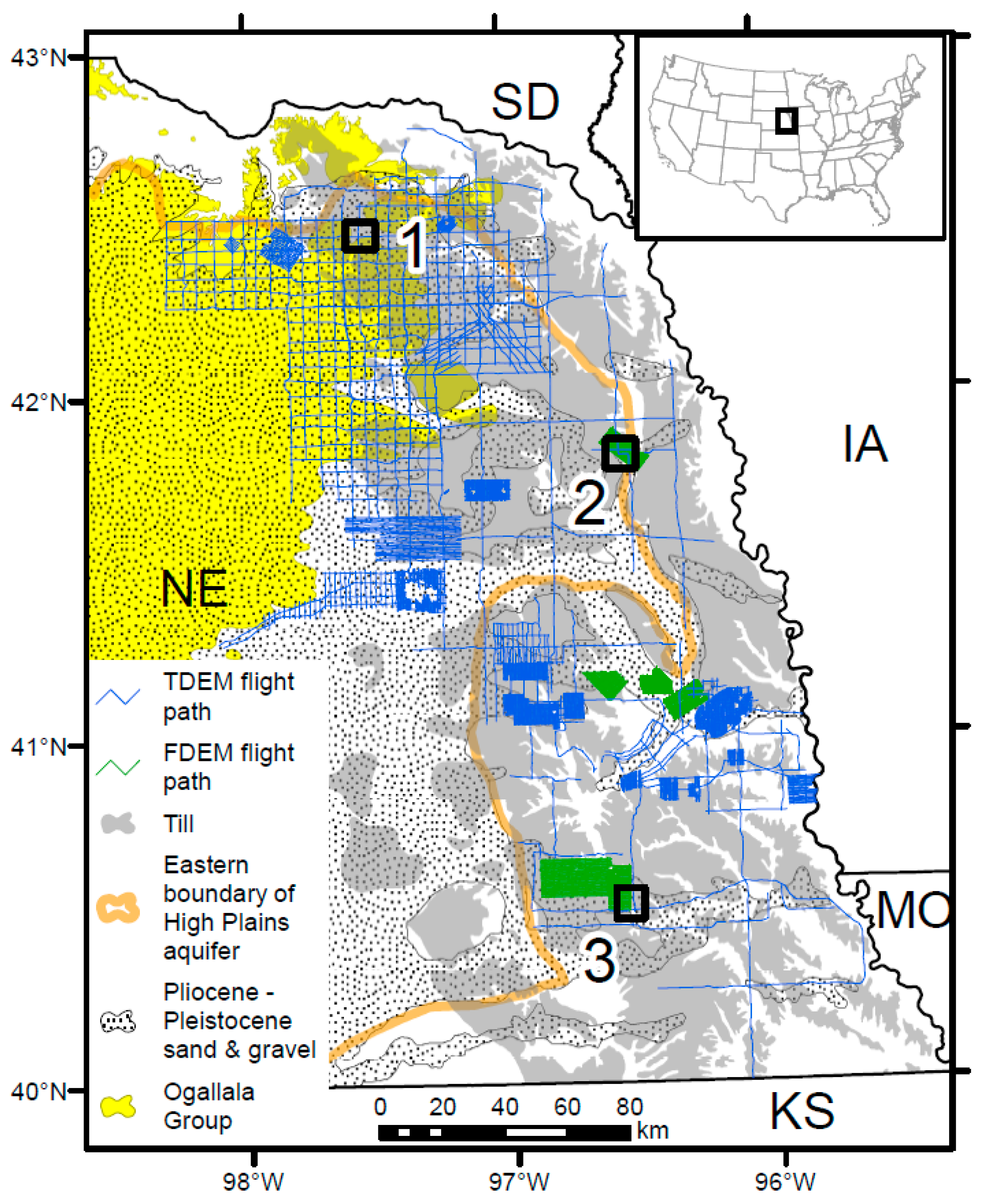
Eastern Nebraska lies at the margin of the Great Plains of central North America. The margin is a transition zone where upper Neogene to early Pleistocene clastic sediments of the High Plains aquifer (HPA) give way to dominantly fine-grained Laurentide (Pleistocene) glacial deposits (Figure 1). The bedrock surface comprises Pennsylvanian and Permian shale and limestone in the southeast and Cretaceous sandstone, siltstone, shale, and chalk in the northeast. Bedrock units function mostly as confining units; however, aquifers are present locally within sandstone and chalk. The HPA is the principal aquifer in the region. It comprises the Neogene Ogallala Group and Pliocene to Pleistocene sands and gravels. The Ogallala consists predominantly of semi-consolidated silts, sands, and minor gravels and it is separated from older Paleozoic to Mesozoic strata by a widespread erosional unconformity [41]. Sheet-like sand bodies and thin mudstones were deposited in broad alluvial megafan systems associated with the erosional unroofing of the Rocky Mountains to the west [42,43,44]. These strata are erosionally and unconformably overlain on the far eastern margin by Pre-Illinoian glacial deposits associated with Laurentide (Pleistocene) glaciations of North America. Glacial deposits consist dominantly of clay-rich diamicton and stratified silts and fine sands. Secondary aquifers within the glacial region are associated with localized sand and gravel deposits from outwash systems, buried valleys, and Holocene alluvium. Buried valley aquifer units are common and were deposited by either (1) bedload-dominated streams within moderately wide (10 km), linear valleys atop bedrock, or (2) glaciofluvial systems and subglacial streams within narrow (~1–3 km), linear to slightly sinuous valleys encased within fine-grained glacial deposits [45]. Most of the landscape is blanketed by one to several layers of loess of variable thickness. Case studies presented herein are from three sites in eastern Nebraska, the details of which are presented later in the paper.
3. Hydraulic Methods
Hydraulic head data were collected and interpreted by three different means described below. In all cases, analyses of hydraulic data was completed prior to the analysis of AEM data. The hydraulic data are therefore unbiased in regard to the hydrostratigraphic interpretations.
An observation well is located at site 1 (Figure 1) and is equipped with a pressure transducer to collect a continuous, long-term record of water levels. This data is used by local groundwater management agencies to monitor changes in groundwater availability and alert officials to potential impacts of pumping or drought on local water supplies. Readings were recorded every 8 h and were converted to depth below the measuring point, which is the top of the PVC well casing. These depths were subtracted from the surveyed elevation of the well casing to determine water elevation. Anomalous water levels recorded during sampling events were removed from the datasets. The transducer was downloaded annually, and quality assurance was performed comparing manual water level measurements to transducer readings. The hydrograph for this site dates to 2005, but two data gaps exist as a result of equipment malfunctions.
A 94-h, constant-rate pumping test was performed from 6–10 April 2009 at site 2 (Figure 1). The pumping well was a municipal well screened from 59.4–68.6 m below ground surface (bgs.). The mean pumping rate was 2.81 × 10⁻² m3/s, but varied between 2.71 × 10⁻² and 2.84 × 10⁻² m3/s due to variations in the pump motor and well hydraulics. Eight observation wells were installed in three nests oriented along a north–south line. Only the six wells in which water levels responded to pumping are described here. Nest 1 was 28 m from the pumping well and consisted of wells with screened intervals 40.5–52.4 and 61.0–70.1 m bgs. Nest 2 was 42 m from the pumping well and consisted of wells screened 39.6–51.8 and 59.4–68.6 m bgs. Nest 3 was 63 m from the pumping well and consisted of wells screened 41.1–53.3 and 59.4–68.6 m bgs. Hydraulic heads were recorded using pressure transducers installed in observation wells as well as periodic manual measurements. The sampling rate of the transducers decreased logarithmically from 0.1 min at the start of the test to 60 min at the end of the test.
A previous study provides a combined water table/potentiometric surface map for site 3 using data from 210 wells [46]. Water levels represent measurements made in observation wells as well as those reported by drillers in well registration records. To increase the density of data coverage, the database includes static water level readings from different periods. Use of data from different years is justified because long-term changes in water levels for this area are generally less than 1.5 m [47]. Water levels measured during the irrigation season (June through September) and those that were highly anomalous compared to neighboring wells were discarded. The surface was interpolated using the inverse distance weighting method at 100 m grid spacing. Contours generated from the raster surface were manually smoothed in some areas, but the overall shape and form of the surface was retained.
4. Airborne Electromagnetic (AEM) Methods
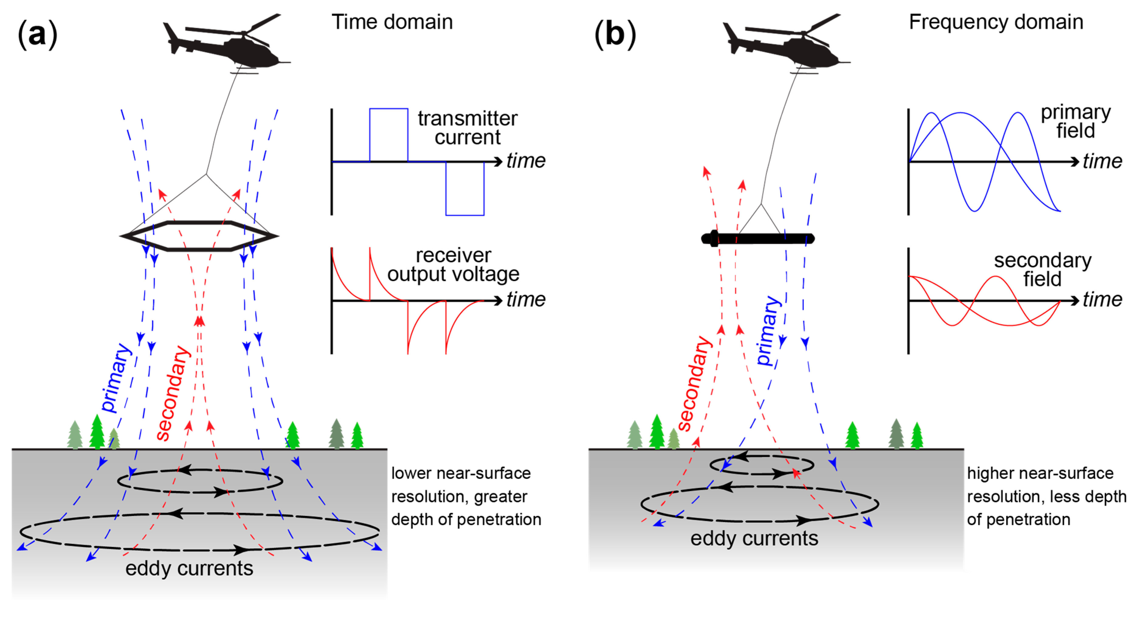
AEM operates on the principal of electromagnetic induction, yielding information on the electrical properties of the subsurface. An AEM system consists of transmitter and receiver coils suspended from an aircraft. The transmitter coil generates a primary magnetic field that interacts with the ground to induce eddy currents, which generate a secondary magnetic field (Figure 2). The receiving coil measures the induced voltage brought about by the secondary field. Resistivity-depth profiles are generated through numerical inversion, providing 2D and 3D visualization of the conductivity structure of the subsurface. AEM is highly sensitive to human infrastructure such as pipelines, transmission lines, fences, and buildings, so proper data filtering and processing is essential for correct interpretation [48]. Numerical inversion is non-unique; many solutions can equally fit the data within the range of error. To provide constraints on the inversions, borehole resistivity logs can be used to estimate minimum and maximum resistivity values for the survey area.
The electrical properties of the Earth depend on a variety of factors: Degree of saturation, clay content, sediment texture, porosity, water chemistry, and metallic mineralization [49]. The relationship between the electrical and hydrological properties of aquifers are non-unique and variable. In most aquifers, however, host sediment or rock is typically nonconductive (sand, sandstone, limestone); variations in electrical conductivity primarily relate to water chemistry and clay content. If groundwater is fresh, electrical conductivity is strongly correlated with clay content [24,50,51,52]. Nevertheless, auxiliary information is necessary to verify such relationships.
There are two types of AEM systems: Frequency domain (FDEM) and time domain (TDEM) (Figure 2). FDEM systems generate a sinusoidal field and operate continuously at several fixed frequencies. Lower frequencies are sensitive to greater depths. The secondary field is measured in a receiver coil at a set distance from the transmitter. A FDEM system consists of several coil pairs mounted in a single instrument. FDEM generally achieves good near-surface resolution, but the depth of investigation is more limited than TDEM.
The FDEM system used in the present study was the RESOLVE system [53], which operated between 0.2 and 140 kHz and was towed approximately 30 m beneath a helicopter at a height of 30 m above ground. Survey speed was approximately 30 m/s and soundings were made every 3 m along flight lines, which were spaced ~280 m apart [53,54]. The survey footprint of the system is approximately 100 m, but footprint size varies with frequency, survey altitude, and resistivity [55,56]. Geophysical inversion of this dataset [53,54] was accomplished using a regularized least-squares inversion algorithm in the program EM1DFM [57,58]. This 1D, layered-earth model fits a response to the data by minimizing the objective function (Φ) given as follows:
where φd is a sum-of-squares measure of data misfit and φm is the model-structure component of the objective function, which is a measure of model simplicity. β is a tradeoff parameter that determines the balance between data misfit and model structure. The optimal value of β was determined using an automated procedure known as generalized cross-validation (GCV). GCV was chosen only after evaluating multiple inversions of the same data using different methods for determining β [57]. Further details on the procedures used to select inversion parameters are in a published report [54]. Resistivity-depth models containing 25 layers were produced for each sounding point in the study area (Figure 3). Geological features in the study area are larger than the FDEM system footprint, so the one-dimensional algorithm, although it approximates the conductivity value within the sensitive volume of the subsurface, is justifiable. The depth of investigation (DOI) [59] varied from ~55–75 m. Those depths exceeding the DOI were masked in the final resistivity-depth sections. The vertical resolution decreases with depth from 1 m near the surface to 9 m at depths ~70 m below the surface (Figure 3).
A TDEM system operates by executing an abrupt turn-off of an electrical current in a large loop and recording the secondary field in the receiving coil using several time gates (Figure 2). Termination of the current causes the secondary EM field to dissipate and decay, which is measured as voltage in the receiver. Each sounding is represented by a curve describing the rate of decay of the magnetic field. Numerical inversion of the sounding curves produces a resistivity-depth model of the subsurface. TDEM generally provides reduced near-surface resolution compared to FDEM, but it is sensitive to greater depths.
A dual moment TDEM system was used in this study [60]. This system uses low and high energizing magnetic moments. The lower current achieves faster field termination, improving near-surface resolution. The higher current is used to resolve targets at greater depths. The TDEM data herein are from surveys flown in 2014 using the SkyTEM 508 system [61] and in 2016 using the SkyTEM 304M system [62]. The 508 system consists of an eight-turn transmitting coil with an area of 536 m2. A peak current of 8.6 A is passed through one turn of wire for low-moment measurements. A peak current of 127 A is passed through all eight turns of wire for high-moment measurements. The 508 system flew at an average height of 43.1 m above ground and an average air speed of 80.5 km/h. The 304M system consists of a four-turn transmitting coil with an area of 337 m2. A peak current of 9 A is passed through one turn of wire for low-moment measurements, and a peak current of 120 A is passed through all four turns for high-moment measurements. The 304M system flew at an average height of 36.4 m and an average air speed of 100.5 km/h. Soundings were collected every ~57 meters for the 508 survey, and every ~72 m for the 304M survey. The receiving coil for both systems has an effective area of 105 m2 and is offset from the transmitter at a position where the sum of all primary fields is zero, maximizing its sensitivity to the secondary field. Flight height, tilt, position, and velocity were collected continuously during flight using laser altimeters, inclinometers, and differential global positioning systems. System footprint depends on bandwidth, height, electrical conductivity, and numerical regularizations in the inversion [63,64]. To minimize over-smoothing and system footprint, the regularization values were carefully selected by comparing TDEM results to boreholes and data residuals.
One-dimensional, resistivity-depth models were generated for each sounding using a spatially constrained inversion (SCI) method [65]. This method derives model parameters from nearest neighbors. The inversion problem is given as follows:
where G is the Jacobian matrix containing the partial derivatives of the data and R describes the spatial constraints or links between soundings both along and across flight lines. The term δmtrue is the difference between the true model and an arbitrary reference model. The term δdobs is the difference between the observed data and the reference model, δr are the constraints, eobs is the error associated with the observed data, and er is the error on the constraints.
This method provides a laterally smooth, quasi-three-dimensional resistivity model with sharp layer boundaries that respect the geological realities of sedimentary deposits (Figure 3). The SCI resistivity-depths models contain 29 layers. Inversion of the 508 system data used a starting resistivity of 10 ohm-m and input parameters for vertical and lateral constraints were set to 2 and 1.3, respectively. Inversion of the 304M system data used a starting resistivity of 10 ohm-m and constraint levels were set to 2.7 vertically and 1.6 laterally. Vertical resolution of the resistivity-depth model for the 508 system data is 5 m for the top layer. Vertical resolution of the model for 304M system data is 3 m for the top layer. For both models, layer thickness increases by a factor of 1.08 for each successive layer. The average DOI [63,64] of the 508 system survey is 198 m and 261 m for the most and least conservative estimates, respectively. The average DOI of the 304M system survey is 153 m and 198 m for the most and least conservative estimates, respectively. Additional details of the SCI approach for these data are in previous reports [61,62].
5. Results
5.1. Site 1: Wausa
Site 1 is located near the Village of Wausa in northeastern Nebraska, ~4 km north of the erosional limit of the Ogallala Group (Figure 1). The area has sparse irrigation and limited groundwater availability. A borehole log from the site shows bedrock at a depth of 74 m, consisting of Cretaceous Pierre Shale. Unconsolidated Quaternary sediments comprise, in succession, 37 m of interbedded sand and clay, 31 m of diamicton, and 6 m of loess.
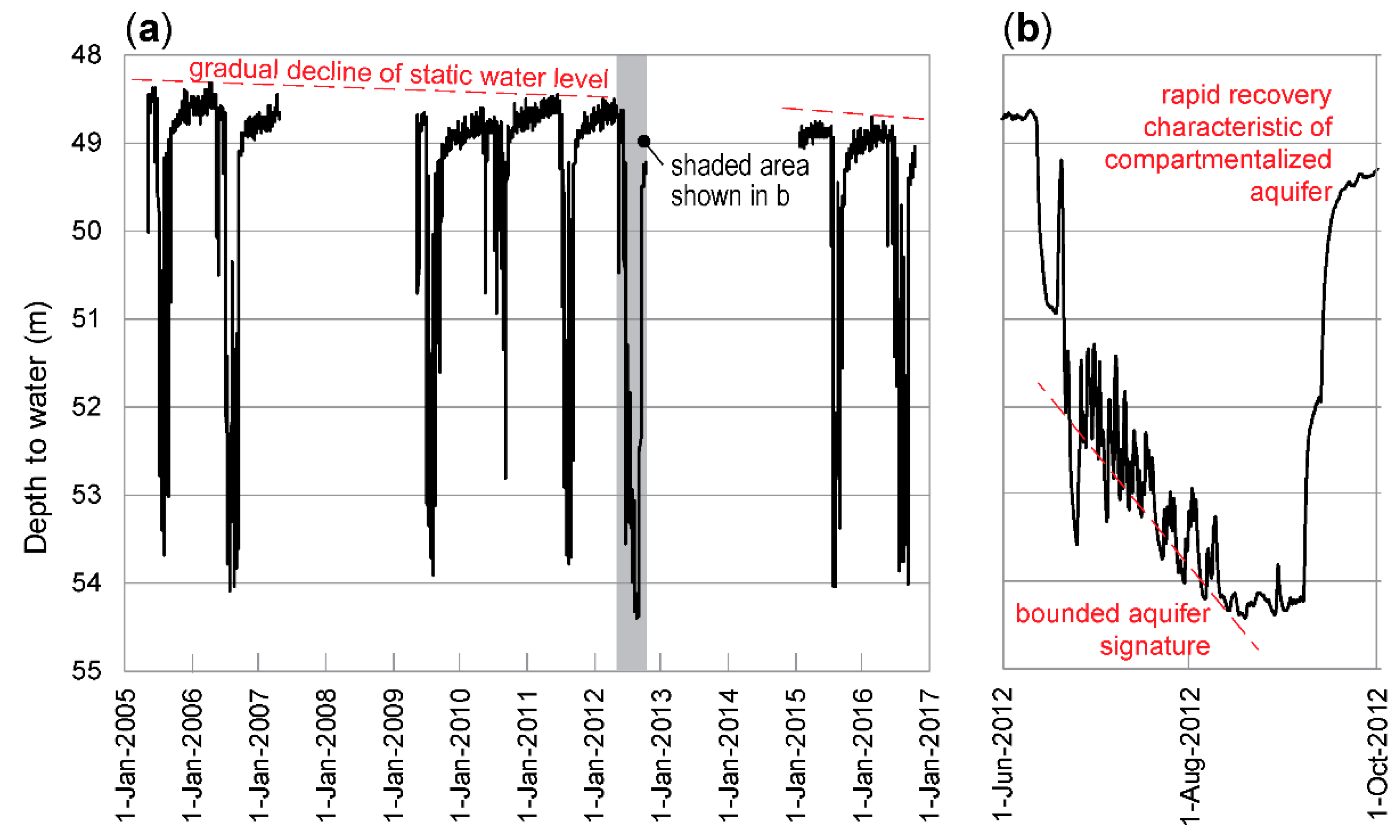
The hydrograph collected at the Wausa site contains records of pumping-induced changes in water level during annual irrigation seasons, which typically lasts from late June to early September (Figure 4). Water-levels typically drop 5–5.5 m at the observation well site during this season (Figure 4a). Smaller fluctuations are superimposed on the overall drawdown pattern, likely representing the cycling on and off of irrigation wells (Figure 4b). There is a slight downward trend in the depth to which water levels recover from pumping each year. The water-level changes at this site probably reflect combined effects of the five nearby irrigation wells. Three of these wells are part of a series (they all supply water to the same irrigation system) and are located between 873–1037 m from the observation well. The other two wells are located 1224 m and 1298 m from the observation well.
Figure 4b shows that the 2012 pumping season began around 11 June and lasted until 7 September, or about 87 days. The general trend of drawdown falls on a straight line beginning about 10 days after pumping began and lasting until approximately day 68 (Figure 4b). Between days 68 and 87, drawdown fell along a generally horizontal line. At day 87 a sudden, rapid recovery of the water level began and lasted about 13 days, stabilizing around 20 September. The duration of the recovery period was only about 15% of the duration of the pumping period.
Examination of long-term, continuous hydrographs from observation wells can yield information about aquifer dynamics, response to pumping, recharge characteristics, and boundary conditions [66]. The segment of the hydrograph where drawdown vs. time approaches a straight line is indicative of the characteristics of the aquifer (Figure 4b). Previous studies have shown that such a pattern is distinctive of compartmentalized aquifers or those in which all sides are bounded by impermeable barriers [66,67]. The straight-line segment begins after the cone of depression reaches the boundaries in all directions. The rapid recovery period is also indicative of a compartmentalized aquifer. In an unbounded aquifer, the recovery period is typically several times longer than the pumping period [66]. The recovery period in the Wausa observation well is a small fraction of the total pumping period. This is further evidence that the aquifer is bounded on all sides.
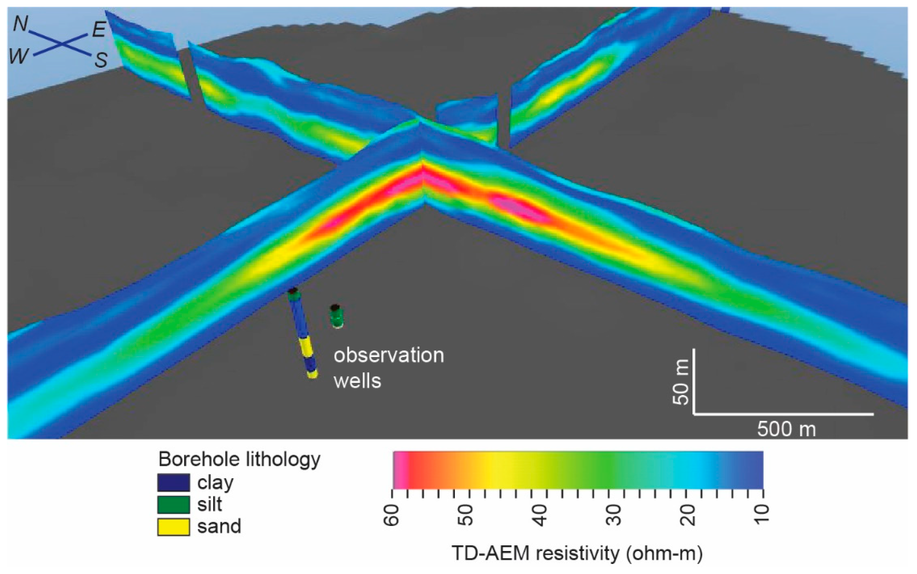
A reconnaissance TDEM survey was conducted in 2016 in northeastern Nebraska with the SkyTEM 304M system. Survey lines were flown approximately 5 km apart along north–south and east–west grid traverses. Two of these lines intersect near the observation well at the Wausa site (Figure 1). The nearest line is 400 m north of the observation well. Resistivity ranges from ~3–64 ohm-m in the resistivity-depth profiles at this site (Figure 5). A zone of high resistivity (45–64 ohm-m) exists at the intersection of the two profiles. The zone is ~30 m thick and 1300 m wide in the east-west direction, and 1800 m wide in the north-south direction. The zone terminates in all four cardinal directions, although the exact dimensions of the feature cannot be resolved because the flight-line spacing exceeds the dimensions of the geologic feature.
The zone of high resistivity corresponds to an interval of very fine to coarse, gravelly sand encountered in the geologic test hole drilled at the site of the observation well. The conductive material above the sand layer corresponds to clay-rich till overlain by loess. The conductive unit below the sand layer corresponds to silty clay with layers of very fine to coarse, gravelly sand. The bottom 7 m of the test hole penetrated shale bedrock.
The shape of the drawdown curve, along with shape of the high resistivity zone in the geophysical profiles, strongly suggest that the irrigation wells in this area withdraw groundwater from a bounded, compartmentalized aquifer. The 12-year record of annual drawdown and recovery shows a slight downward trend in the static water level, suggesting that groundwater is supplied to the pumping wells primarily from water in storage and that recharge to the aquifer is limited.
5.2. Site 2: Oakland
Site 2 is located near the City of Oakland at the site of a municipal water supply well. The well is located in an upland area adjacent to a river valley. The valley contains a series of terraces that lie 12 m above the modern valley floodplain. Borehole logs at the well site indicate two unconsolidated sand and gravel aquifers separated by a 1.5-m thick confining unit consisting of clay and silt. A 9-m thick clay unit separates the bottom of the lower aquifer from the top of a sandstone unit in the Cretaceous Dakota Group.
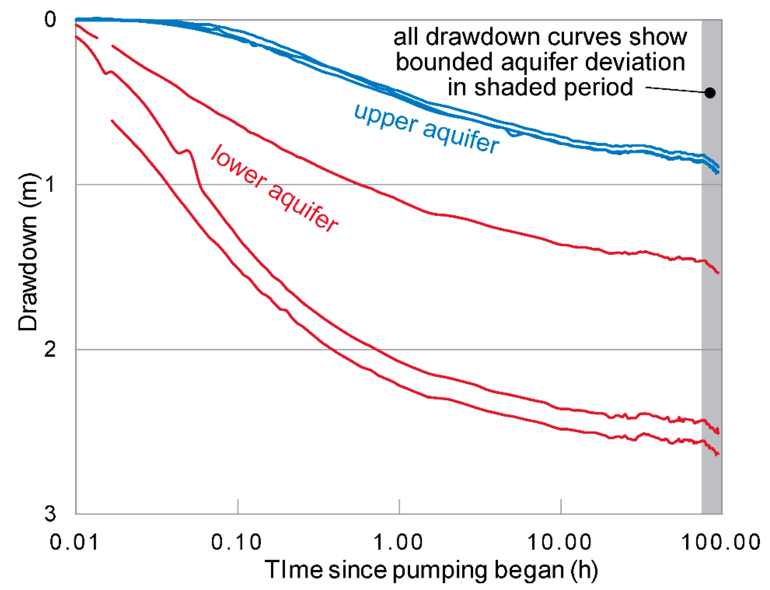
Plots of drawdown versus time for the pumping test observation wells show an initial time of rapid, relatively steady rate of drawdown (0.01 to 0.3 h); a time in which the rate of drawdown steadily decreases (0.3 to 17 h); a time in which drawdown is very slow or stationary (17–75 h); and a late time in which the rate of drawdown increases sharply to 8 cm/day (75–94 h) (Figure 6). Water levels were still decreasing at the end of the pumping period. Wells screened in the lower aquifer (the aquifer in which the pumping well is screened) all showed greater drawdown than the wells screened in the upper aquifer.
In a confined aquifer of infinite extent, a semi-logarithmic plot of drawdown versus time would form a straight line [68]. The drawdown and recovery curves in this pumping test behave initially as would a confined aquifer. After 20 min, however, rates of drawdown decline, forming a curved line typical of a leaky confined aquifer. Further evidence of leakage from the upper to the lower aquifer through the confining unit is shown in the response of the upper aquifer, which declines a total of ~1 m during the pumping period.
Between 75–94 h after pumping began, the drawdown curves deviate from the predicted response of a leaky aquifer (Figure 6). The sharp increase in the rate of drawdown in all wells suggests that the cone of depression reached an impermeable boundary. This boundary appears to affect water levels in all of the wells equally and at the same time, so the direction of this boundary cannot be ascertained from hydraulic data alone.
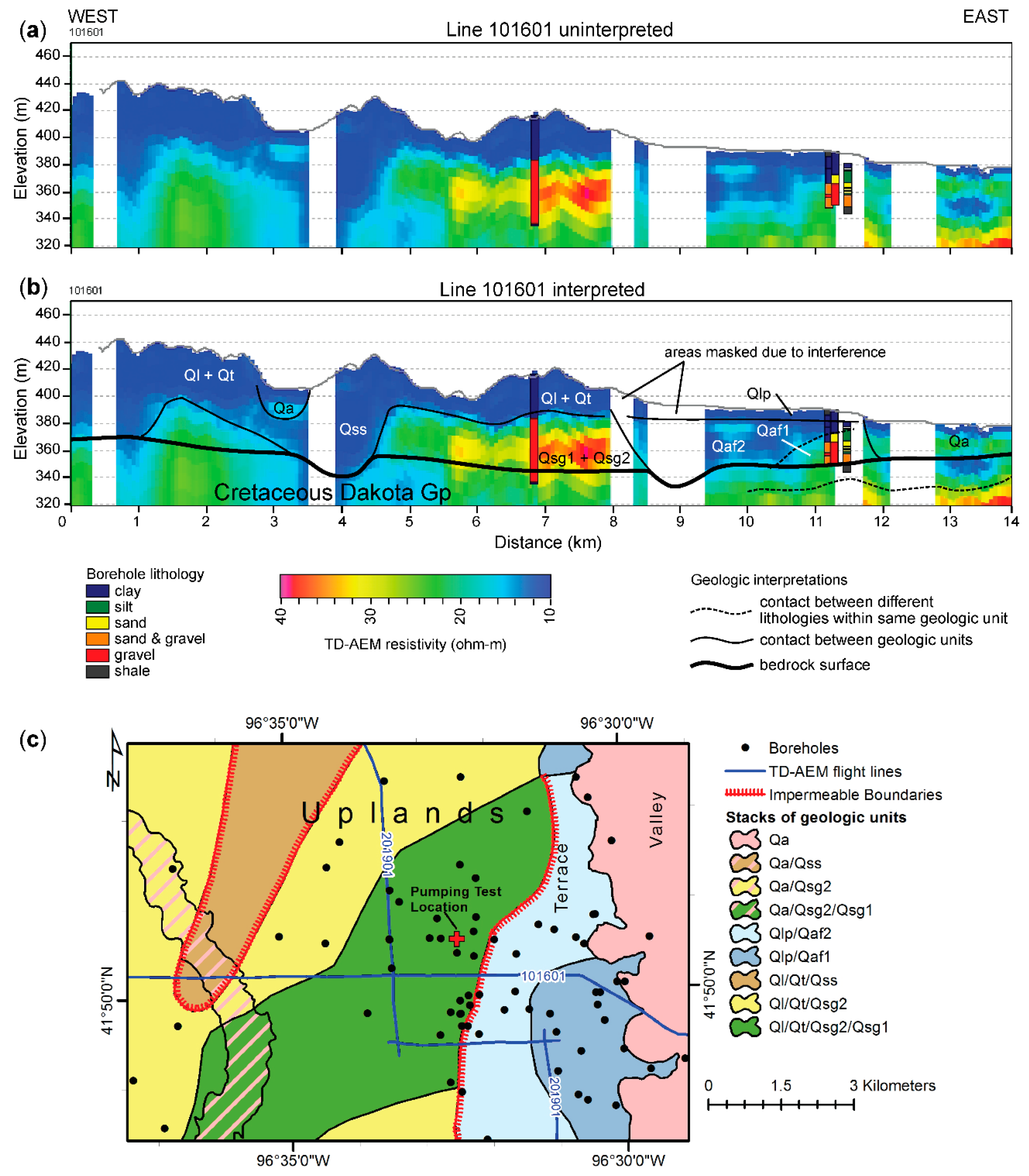
A reconnaissance TDEM survey was conducted in 2014 in northeastern Nebraska with the SkyTEM 508 system (Figure 7). Two survey lines were flown through the Oakland site. The depth of investigation of the TDEM surveys was sufficient to penetrate the entire thickness of the Quaternary sediments and into the underlying Cretaceous bedrock below 80 m. TDEM profiles show a zone of high (~25–40 ohm-m) resistivity bounded to the east and west by low resistivity (<15 ohm-m) units. The high-resistivity unit is 3.5 km wide and 40 m thick. A FDEM survey was also flown over the study site, but it was unsuccessful at imaging to the depths of the units of interest and is therefore not shown here.
Analysis of borehole logs shows that the high resistivity unit corresponds to the multi-layer aquifer at the site (Figure 7). AEM does not resolve the two layers of the aquifer, but these units have been identified in borehole logs. The lower aquifer fills a southwest–northeast trending bedrock low. The upper aquifer is more extensive. Low-resistivity units bounding the aquifer correspond to interbedded clay, silt, and clay-rich diamicton. The eastern unit underlies a terrace located on the margin of the river valley. The western unit fills a buried valley under the uplands.
5.3. Site 3: Firth
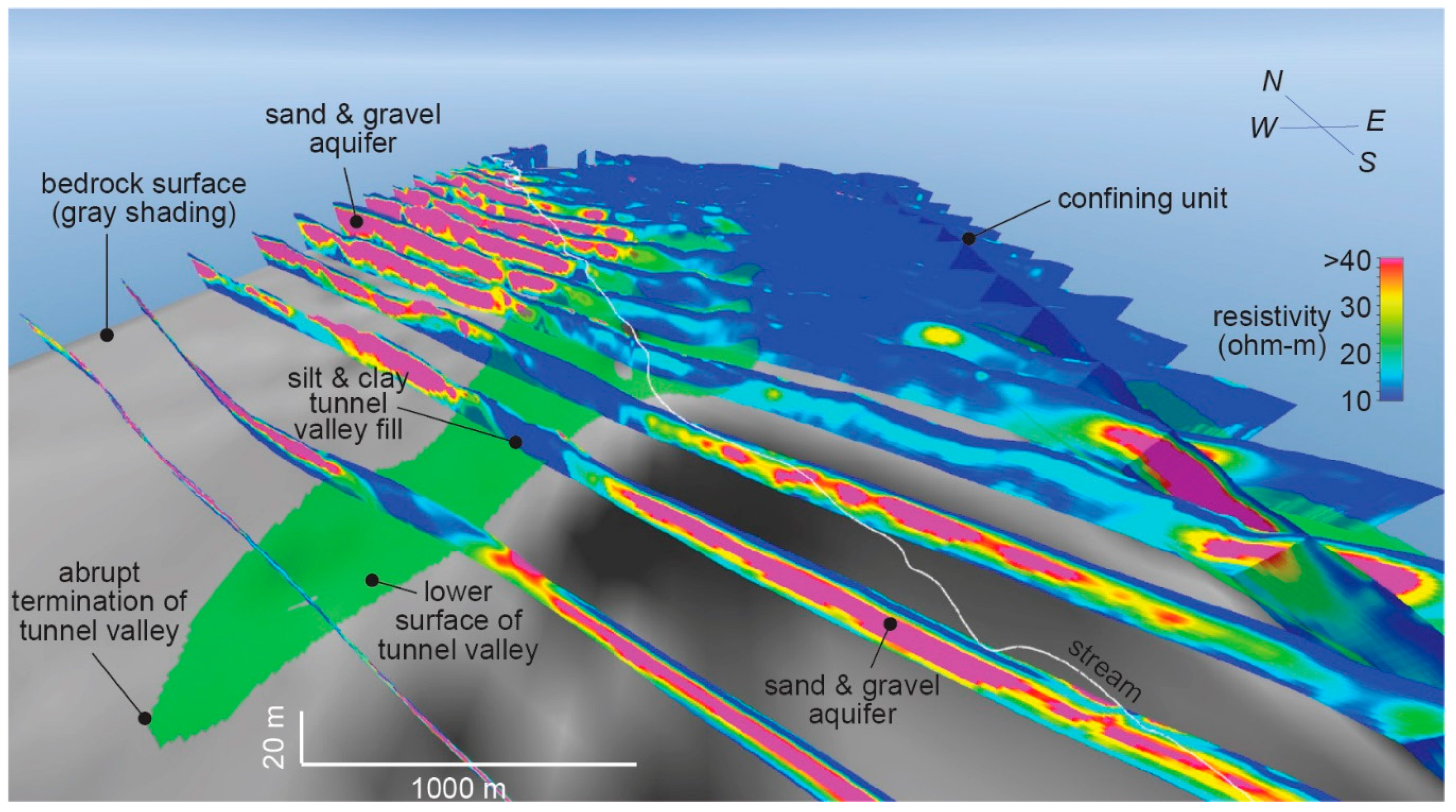
Site 3, near the Village of Firth, is located on the southern margin of a 12-km wide, west–east trending buried valley that extends at least 180 km eastward of the margin of the High Plains aquifer [45]. The paleovalley fill contains abundant sand and gravel, forming an important aquifer in the region. The aquifer is locally truncated by younger deposits associated with subglacial tunnel valleys [45]. These valleys are narrow (1–3 km), steep-sided (10°–30°), and linear to slightly sinuous. Some of these valleys are filled with sand and gravel, others with silt, clay, and diamicton.
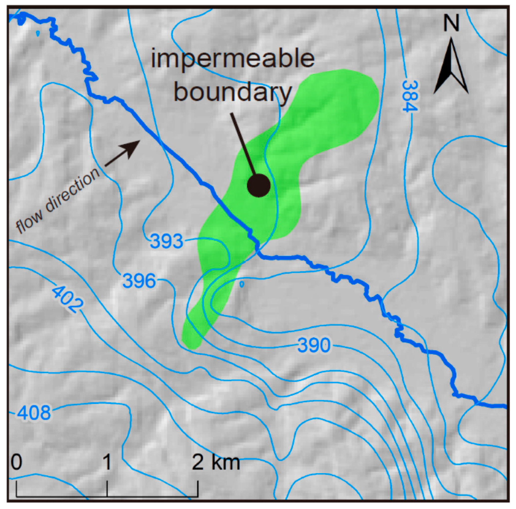
The map of the water table at the Firth site reveals an abrupt change in the hydraulic gradient and groundwater flow direction near the southern margin of a stream valley (Figure 8). The gradient in the northern part of the site is 0.004 toward the east/northeast, but in the southern part, the gradient abruptly increases by a factor of 10, to 0.024, and the direction changes to north/northeast. This change takes place over a distance of <1 km. There are no known large-volume withdrawals of groundwater, recharge sources from large surface water bodies, or other features in this area that would contribute to the observed anomalies. The water table configuration, however, can be explained by the presence of a discontinuous, impermeable or low-permeability boundary in the aquifer.
A low-K unit acts as an impoundment, causing an abrupt variation in the flow gradient and direction at the interface between zones with different properties. Water table contours are closely-spaced within the low-permeability zone and widely-spaced up-gradient of that zone. On the south side of the impermeable boundary, the water table slopes northeast along a gradient that mirrors the topographic surface.
A block-type FDEM survey was flown in 2007. It comprised 52 east–west traverses spaced ~280 m apart and two north–south tie lines 6 km apart. The depth of investigation varies between ~50–80 m, which is sufficient to penetrate the entire thickness of unconsolidated materials above bedrock in the studied area. A detailed, 3D geological model has been presented in previous work [45,46]. Resistivity-depth profiles show a zone of high resistivity (>20 ohm-m) in the southwest and a zone of low-resistivity (<20 ohm-m) in the northeast (Figure 9). A narrow, wedge-shaped body of low resistivity extends southward into the zone of high resistivity. It is continuous in resistivity-depth profiles across the stream valley from north to south, terminating under the uplands ~1 km south of the valley margin.
6. Discussion
Mapping impermeable boundaries and analyzing impacts of those boundaries on groundwater systems are critical to any groundwater investigation. The examples given in this paper show that effective characterization of impermeable boundaries can be achieved by combining hydraulic head analysis with AEM. The examples presented here demonstrate the successful detection of impermeable boundaries with three methods: Analysis of water-level data from continuously monitored wells, pumping test interpretation, and evaluation of a water table map. Furthermore, the boundaries were mapped using three different AEM systems: SkyTEM 508, SkyTEM 304M, and RESOLVE. The wide spacing of the SkyTEM profiles (~5 km) prevented the use of geostatistical modeling because the spacing exceeded the spatial dimensions of the geologic features. With the RESOVLE survey, resistivity contrasts defining the bounding surfaces of the geological features of interest varied from place-to-place, so a cognitive approach, rather than a geostatistical one, was used to map the area [45].
Factors other than lithology can influence AEM resistivity, and electrically conductive units need not be impermeable. A zone of electrically conductive water within an aquifer can have a similar appearance to a clay-rich geological body [25]. Although salinity mapping may be of concern in some hydrogeologic studies, in the analysis of hydrostratigraphic units, factors that influence permeability and groundwater flow are of chief concern. It is therefore imperative to determine what characteristics are being resolved by an AEM survey. Data on groundwater levels will typically have a low spatial density compared to borehole lithology data. Ideally, one or more pumping tests would be performed in the vicinity of an impermeable boundary to derive quantitative data on hydrogeologic properties and to determine the time lag between the onset of pumping and the intersection of the water table with the boundary. Pumping tests are time-intensive and costly to perform. Continuous monitoring of hydraulic heads is also costly, and water-level observation wells are often sparse. For these reasons, borehole data will remain an essential part of the total data integration of an AEM study, and geostatistical methods should prove useful for integrating sparse measurements with dense geophysical data to generate 3D realizations of hydrogeologic properties and their associated uncertainties. Complementing these data with hydraulic head measurements has clear advantages for hydrostratigraphic interpretation. Furthermore, the locations of impermeable boundaries detected in hydraulic head analyses could be used to condition geostatistical models so that the maps exactly reproduce the boundaries at the appropriate locations [31]. This conditioning could also ensure that the conductive units are mapped as impermeable geologic bodies juxtaposed against permeable aquifer materials rather than zones of saline groundwater or bodies of rock or sediment with electrically conductive properties that are not necessarily impermeable.
Hydraulic head analysis can aid in the hydrostratigraphic interpretation of AEM in areas of cultural noise. AEM data is especially sensitive to coupling and noise from the influence of man-made infrastructure such as powerlines, pipes, buildings, and other objects [48,65]. Data affected by such interference needs to be culled from the dataset. This is a necessary step in data processing, and it results in gaps in the final resistivity-depth profiles. An example of an area where AEM data was removed due to interference is shown at the Oakland site (Figure 7). The area corresponds to the location of the impermeable boundary. There are no boreholes in the area of the removed AEM data. As a result, the gap creates some uncertainty in the hydrostratigraphic interpretation of the AEM. The pumping test results help to address this uncertainty by showing clear evidence of an impermeable boundary.
The design of an AEM survey (target depths, flight line spacing, orientation) should take into account any hydraulic head data that detect the presence of an impermeable boundary. Ideally, closely spaced flight lines allow for the construction of 3D models, such as the one at Firth (Figure 9). Reconnaissance surveys successfully imaged the impermeable boundaries at Wausa and Oakland (Figure 5 and Figure 7), but due to the widely spaced flight lines, mapping had to be carried out using boreholes. At Wausa, boreholes are too sparse to conduct any additional mapping. Nevertheless, reconnaissance surveys may be useful in very large investigations if flight lines are carefully selected to pass over geologic features of interest. In this way, hydraulic head data, especially water table maps and continuously monitored wells, can be used to design such surveys.
Another reason to incorporate hydraulic head analysis into an AEM survey relates to the vertical resolution of AEM. Horizontal resolution is vastly better than that of boreholes. However, vertical resolution of AEM is quite low compared to boreholes, so detecting thin confining units within thick aquifer bodies may not be possible. The thin, leaky confining unit at Oakland is detectable in the pumping test data, but resistivity-depth profiles do not provide any evidence of this layer. Borehole logs and pumping test data are necessary to resolve these vertical details, and integrating these data with AEM through geostatistical modeling presents a promising avenue for future research [37,38].
Glacial deposits are geologically complex and heterogeneous [69,70]. Boundaries between aquifers and confining units are numerous in glacial aquifers, so mapping them is critically important for the development and management of groundwater supplies and for predicting the fate and transport of contaminants in the subsurface. This study shows the detection and mapping of a variety of impermeable boundaries, from those that surround fully compartmentalized aquifers to those that are localized and discontinuous within regional aquifer systems. Hydraulic head analysis, coupled with AEM and supporting geological data, presents an ideal technique for detecting and mapping impermeable boundaries at a variety of scales in highly heterogeneous glacial deposits.
7. Conclusions
Impermeable boundaries can be detected through the traditional analysis of hydraulic head data from monitoring wells, pumping tests, and water table maps. However, it is difficult or impossible to map the extent and geometry of these boundaries from head data alone. Inversion of AEM data results in non-unique resistivity-depth models. Furthermore, the relationship between resistivity and hydrogeologic properties is not universal and can vary depending on many factors. Because of this non-uniqueness, supporting data is essential to interpreting AEM. Although boreholes are essential for constraining geologic interpretations, hydraulic head analysis provides direct evidence of the hydrostratigraphic function of geologic units and is therefore key to making the correct interpretation of groundwater flow boundaries. AEM provides details on the orientation, thickness, extent, and relationships between hydrostratigraphic units, which are not provided by hydraulic head data alone.
This study demonstrates how impermeable boundaries can be detected from analysis of hydraulic heads and then verified and mapped using airborne electromagnetics (AEM.) Both reconnaissance and block-type AEM surveys are useful, depending on the scale of the investigation, scope of work, and cost limitations.
A fully bounded, closed aquifer system was detected at the Wausa site using hydraulic head changes from a continuously monitored well. This analysis was done on drawdown and recovery curves resulting from pumping of nearby irrigation wells. A reconnaissance AEM survey flown over the site revealed a zone of high resistivity <2 km wide that terminates in all directions. At the Oakland site, a 94-h pumping test revealed an impermeable boundary nearby, but the direction of the boundary could not be ascertained from the data. A reconnaissance AEM survey reveals a 3-km wide impermeable boundary beneath a valley terrace, separating the aquifer from a stream. A water table map of the Firth site shows anomalous horizontal gradients and orientations, which can be interpreted as evidence of an impermeable boundary. 3D mapping from a block AEM survey verifies this interpretation, revealing a 1-km wide, wedge-shaped, discontinuous body of conductive material penetrating the aquifer.
Funding
AEM data collection, pumping test, and water-level monitoring was funded through various projects by Nebraska’s Natural Resources Districts, with additional funding from the Nebraska Natural Resources Commission and the Nebraska Environmental Trust. AEM research by the author was funded by Nebraska’s Natural Resources Districts and the Nebraska Natural Resources Commission (Water Sustainability Fund), grant number 4164. The author’s research program is supported by the U.S. Department of Agriculture National Institute of Food and Agriculture (Hatch project NEB-21-177, accession number 1015698) and the Daugherty Water for Food Global Institute at the University of Nebraska.
Acknowledgments
The author thanks Susan Olafsen-Lackey, Katie Cameron, Amber Fertig, and Levi McKercher for their assistance with data compilation and graphics.
Conflicts of Interest
The author declares no conflict of interest. The funders had no role in the design of the study, in the analyses or interpretation of data, in the writing of the manuscript, or in the decision to publish the results. The Lower Elkhorn Natural Resources District (one of the funding agencies) was responsible for the collection of water-level data shown in Figure 4.
References
- Eaton, T.T. On the importance of geological heterogeneity for flow simulation. Sediment. Geol. 2006, 184, 187–201. [Google Scholar] [CrossRef]
- Blouin, M.; Martel, R.; Gloaguen, E. Accounting for aquifer heterogeneity from geological data to management tools. Groundwater 2013, 51, 421–431. [Google Scholar] [CrossRef] [PubMed]
- Ferris, J.G. Hydrology. In Ground Water; Wisler, C.O., Brater, E.F., Eds.; Wiley & Sons: New York, NY, USA, 1959. [Google Scholar]
- Van der Kamp, G.; Maathuis, H. The Unusual and Large Drawdown Response of Buried-Valley Aquifers to Pumping. Groundwater 2012, 50, 207–215. [Google Scholar] [CrossRef] [PubMed]
- Fleckenstein, J.H.; Niswonger, R.G.; Fogg, G.E. River-aquifer interactions, geologic heterogeneity, and low-flow management. Groundwater 2006, 44, 837–852. [Google Scholar] [CrossRef] [PubMed]
- Irvine, D.J.; Brunner, P.; Franssen, H.-J.H.; Simmons, C.T. Heterogeneous or homogeneous? Implications of simplifying heterogeneous streambeds in models of losing streams. J. Hydrol. 2012, 424, 16–23. [Google Scholar] [CrossRef] [Green Version]
- Shaver, R.B.; Pusc, S.W. Hydraulic barriers in Pleistocene buried-valley aquifers. Groundwater 1992, 30, 21–28. [Google Scholar] [CrossRef]
- Raiber, M.; Webb, J.; Cendón, D.; White, P.; Jacobsen, G. Environmental isotopes meet 3D geological modelling: Conceptualising recharge and structurally-controlled aquifer connectivity in the basalt plains of south-western Victoria, Australia. J. Hydrol. 2015, 527, 262–280. [Google Scholar] [CrossRef]
- Butler, J.J. Pumping tests for aquifer evaluation—Time for a change? Groundwater 2009, 47, 615–617. [Google Scholar] [CrossRef] [PubMed]
- Ferris, J.G.; Knowles, D.B.; Brown, R.H.; Stallman, R.W. Theory of Aquifer Tests; U.S. Geological Survey: Reston, VA, USA, 1962; p. 174.
- Butler, J.J.; Liu, W.Z. Pumping tests in non-uniform aquifers—The linear strip case. J. Hydrol. 1991, 128, 69–99. [Google Scholar] [CrossRef]
- Kruseman, G.P.; Ridder, N.A. Analysis and Evaluation of Pumping Test Data; International Institute for Land Reclamation and Improvement: Wageningen, The Netherlands, 1990; p. 377. [Google Scholar]
- Strausberg, S.I. Estimating Distances to Hydrologic Boundaries from Discharging Well Data. Groundwater 1967, 5, 5–8. [Google Scholar] [CrossRef]
- Palacky, G.J.; Stephens, L.E. Mapping of Quaternary sediments in northeastern Ontario using ground electromagnetic methods. Geophysics 1990, 55, 1596–1604. [Google Scholar] [CrossRef]
- Bowling, J.C.; Rodriguez, A.B.; Harry, D.L.; Zheng, C. Delineating alluvial aquifer heterogeneity using resistivity and GPR data. Groundwater 2005, 43, 890–903. [Google Scholar] [CrossRef] [PubMed]
- Goutaland, D.; Winiarski, T.; Dubé, J.-S.; Bièvre, G.; Buoncristiani, J.-F.; Chouteau, M.; Giroux, B. Hydrostratigraphic characterization of glaciofluvial deposits underlying an infiltration basin using ground penetrating radar. Vadose Zone J. 2008, 7, 194–207. [Google Scholar] [CrossRef]
- Brosten, T.R.; Day-Lewis, F.D.; Schultz, G.M.; Curtis, G.P.; Lane, J.W. Inversion of multi-frequency electromagnetic induction data for 3D characterization of hydraulic conductivity. J. Appl. Geophys. 2011, 73, 323–335. [Google Scholar] [CrossRef]
- Triantafilis, J.; Ribeiro, J.; Page, D.; Monteiro Santos, F. Inferring the location of preferential flow paths of a leachate plume by using a DUALEM-421 and a Quasi-Three-Dimensional inversion model. Vadose Zone J. 2013, 12. [Google Scholar] [CrossRef]
- Robinson, D.A.; Binley, A.; Crook, N.; Day-Lewis, F.D.; Ferre, T.P.A.; Grauch, V.J.S.; Knight, R.; Knoll, M.; Lakshmi, V.; Miller, R.; et al. Advancing process-based watershed hydrological research using near-surface geophysics: A vision for, and review of, electrical and magnetic geophysical methods. Hydrol. Process. 2008, 22, 3604–3635. [Google Scholar] [CrossRef]
- Siemon, B.; Christiansen, A.V.; Auken, E. A review of helicopter-borne electromagnetic methods for groundwater exploration. Near Surf. Geophys. 2009, 7, 629–646. [Google Scholar] [CrossRef]
- Pellerin, L.; Beard, L.P.; Mandell, W. Mapping Structures that Control Contaminant Migration using Helicopter Transient Electromagnetic Data. J. Environ. Eng. Geophys. 2010, 15, 65–75. [Google Scholar] [CrossRef]
- Kirkegaard, C.; Sonnenborg, T.O.; Auken, E.; Jørgensen, F. Salinity Distribution in Heterogeneous Coastal Aquifers Mapped by Airborne Electromagnetics. Vadose Zone J. 2011, 10, 125–135. [Google Scholar] [CrossRef]
- Jorgensen, F.; Moller, R.R.; Nebel, L.; Jensen, N.-P.; Christiansen, A.V.; Sandersen, P. A method for cognitive 3D geological voxel modelling of AEM data. Bull. Eng. Geol. Environ. 2013, 72, 421–432. [Google Scholar] [CrossRef] [Green Version]
- Gunnink, J.L.; Siemon, B. Applying airborne electromagnetics in 3D stochastic geohydrological modelling for determining groundwater protection. Near Surf. Geophys. 2015, 13, 45–60. [Google Scholar] [CrossRef]
- Costabel, S.; Siemon, B.; Houben, G.; Günther, T. Geophysical investigation of a freshwater lens on the island of Langeoog, Germany—Insights from combined HEM, TEM and MRS data. J. Appl. Geophys. 2017, 136, 231–245. [Google Scholar] [CrossRef]
- Paine, J.G.; Collins, E.W. Identifying Ground-water Resources and Intrabasinal Faults in the Hueco Bolson, West Texas, using Airborne Electromagnetic Induction and Magnetic-field Data. J. Environ. Eng. Geophys. 2017, 22, 63–81. [Google Scholar] [CrossRef]
- Marker, P.A.; Foged, N.; He, X.; Christiansen, A.V.; Refsgaard, J.C.; Auken, E.; Bauer-Gottwein, P. Performance evaluation of groundwater model hydrostratigraphy from airborne electromagnetic data and lithological borehole logs. Hydrol. Earth Syst. Sci. 2015, 19, 3875–3890. [Google Scholar] [CrossRef] [Green Version]
- Barfod, A.A.S.; Møller, I.; Christiansen, A.V.; Høyer, A.-S.; Hoffimann, J.; Straubhaar, J.; Caers, J. Hydrostratigraphic modeling using multiple-point statistics and airborne transient electromagnetic methods. Hydrol. Earth Syst. Sci. 2018, 22, 3351–3373. [Google Scholar] [CrossRef]
- Raingeard, A.; Reninger, P.-A.; Thiery, Y.; Lacquement, F.; Nachbaur, A. 3D geological modelling coupling AEM with field observations. In Proceedings of the 7th International Workshop on Airborne Electromagnetics, Kolding, Denmark, 17–20 June 2018. [Google Scholar]
- Høyer, A.-S.; Jørgensen, F.; Lykke-Andersen, H.; Christiansen, A.V. Iterative modelling of AEM data based on a priori information from seismic and borehole data. Near Surf. Geophys. 2014, 12, 635–650. [Google Scholar] [CrossRef]
- Koltermann, C.E.; Gorelick, S.M. Heterogeneity in sedimentary deposits: A review of structure-imitating, process-imitating, and descriptive approaches. Water Resour. Res. 1996, 32, 2617–2658. [Google Scholar] [CrossRef]
- Fogg, G.E.; Noyes, C.D.; Carle, S.F. Geologically based model of heterogeneous hydraulic conductivity in an alluvial setting. Hydrogeol. J. 1998, 6, 131–143. [Google Scholar] [CrossRef]
- Anderson, M.; Aiken, J.; Webb, E.; Mickelson, D. Sedimentology and hydrogeology of two braided stream deposits. Sediment. Geol. 1999, 129, 187–199. [Google Scholar] [CrossRef]
- De Marsily, G.; Delay, F.; Gonçalvès, J.; Renard, P.; Teles, V.; Violette, S. Dealing with spatial heterogeneity. Hydrogeol. J. 2005, 13, 161–183. [Google Scholar] [CrossRef] [Green Version]
- Huggenberger, P.; Regli, C. A sedimentological model to characterize braided river deposits for hydrogeological applications. In Braided Rivers: Process, Deposits, Ecology, and Management; Sambrook, G.H., Best, J.L., Bristow, C.S., Petts, G.E., Eds.; Blackwell Publishing: Oxford, UK, 2009; pp. 51–74. [Google Scholar]
- Bayer, P.; Comunian, A.; Höyng, D.; Mariethoz, G. High resolution multi-facies realizations of sedimentary reservoir and aquifer analogs. Sci. Data 2015, 2. [Google Scholar] [CrossRef] [PubMed]
- Marini, M.; Felletti, F.; Beretta, G.; Terrenghi, J. Three Geostatistical Methods for Hydrofacies Simulation Ranked Using a Large Borehole Lithology Dataset from the Venice Hinterland (NE Italy). Water 2018, 10, 844. [Google Scholar] [CrossRef]
- Barfod, A.A.S.; Vilhelmsen, T.N.; Jorgensen, F.; Christiansen, A.V.; Straubhaar, J.; Moller, I. Contributions to uncertainty related to hydrostratigraphic modeling using Multiple-Point Statistics. Hydrol. Earth Syst. Sci. 2018, 1–38. [Google Scholar] [CrossRef]
- Ruggeri, P.; Irving, J.; Holliger, K.; Gloaguen, E.; Lefebvre, R. Hydrogeophysical data integration at larger scales: Application of Bayesian sequential simulation for the characterization of heterogeneous alluvial aquifers. Lead. Edge 2013, 32, 766–774. [Google Scholar] [CrossRef]
- Friedel, M.J. Estimation and scaling of hydrostratigraphic units: Application of unsupervised machine learning and multivariate statistical techniques to hydrogeophysical data. Hydrogeol. J. 2016, 24, 2103–2122. [Google Scholar] [CrossRef]
- Gutentag, E.D.; Heimes, F.J.; Krothe, N.C.; Luckey, R.R.; Weeks, J.B. Geohydrology of the High Plains Aquifer in Parts of Colorado, Kansas, Nebraska, New Mexico, Oklahoma, South Dakota, Texas, and Wyoming; U.S. Geological Survey: Reston, VA, USA, 1984; p. 63.
- Seni, S.J. Sand-Body Geometry and Depositional Systems, Ogallala Formation, Texas; Bureau of Economic Geology, University of Texas at Austin: Austin, TX, USA, 1980. [Google Scholar]
- Joeckel, R.M.; Wooden, S.R., Jr.; Korus, J.T.; Garbisch, J.O. Architecture, heterogeneity, and origin of late Miocene fluvial deposits hosting the most important aquifer in the Great Plains, USA. Sedimentology 2014, 311, 75–95. [Google Scholar] [CrossRef] [Green Version]
- Shepherd, R.G. Hydrogeologic significance of Ogallala fluvial environments, the Gangplank. In Recent and Ancient Nonmarine Depositional Environments; Models for Exploration; Ethridge, F.G., Flores, R.M., Eds.; SEPM (Society for Sedimentary Geology): Tulsa, OK, USA, 1981; Volume 31, pp. 89–94. [Google Scholar]
- Korus, J.T.; Joeckel, R.M.; Divine, D.P.; Abraham, J.D. Three-dimensional architecture and hydrostratigraphy of cross-cutting buried valleys using airborne electromagnetics, glaciated Central Lowlands, Nebraska, USA. Sedimentology 2016. [Google Scholar] [CrossRef]
- Korus, J.T.; Joeckel, R.M.; Divine, D.P. Three-Dimensional Hydrostratigraphy of the Firth, Nebraska Area: Results from Helicopter Electromagnetic (HEM) Mapping in the Eastern Nebraska Water Resources Assessment (ENWRA); Conservation and Survey Division, School of Natural Resources, Institute of Agriculture and Natural Resources, University of Nebraska-Lincoln: Lincoln, NE, USA, 2013; p. 100. [Google Scholar]
- Young, A.R.; Burbach, M.E.; Howard, L.M.; Waszgis, M.M.; Joeckel, R.M.; Olafsen-Lackey, S. Nebraska Statewide Groundwater-Level Monitoring Report 2016; Conservation and Survey Division, School of Natural Resources, Institute of Agriculture and Natural Resources, University of Nebraska-Lincoln: Lincoln, NE, USA, 2015; p. 24. [Google Scholar]
- Viezzoli, A.; Jørgensen, F.; Sørensen, C. Flawed Processing of Airborne EM Data Affecting Hydrogeological Interpretation. Groundwater 2013, 51, 191–202. [Google Scholar] [CrossRef] [PubMed]
- Lesmes, D.P.; Friedman, S.P. Relationship between the electrical and hydrogeological properties of rocks and soils. In Hydrogeophysics; Rubin, Y., Hubbard, S.S., Eds.; Springer: Dordrecht, The Netherlands, 2005; pp. 87–128. [Google Scholar]
- Beamish, D. Petrophysics from the air to improve understanding of rock properties in the UK. First Break 2013, 31, 63–71. [Google Scholar]
- Christiansen, A.V.; Foged, N.; Auken, E. A concept for calculating accumulated clay thickness from borehole lithological logs and resistivity models for nitrate vulnerability assessment. J. Appl. Geophys. 2014, 108, 69–77. [Google Scholar] [CrossRef]
- Barfod, A.A.S.; Møller, I.; Christiansen, A.V. Compiling a national resistivity atlas of Denmark based on airborne and ground-based transient electromagnetic data. J. Appl. Geophys. 2016, 134, 199–209. [Google Scholar] [CrossRef]
- Smith, B.D.; Abraham, J.A.; Cannia, J.C.; Steele, G.V.; Hill, P. Helicopter Electromagnetic and Magnetic Geophysical Survey Data, Oakland, Ashland, and Firth Study Areas, Eastern Nebraska, March 2007; U.S. Geological Survey: Reston, VA, USA, 2008; p. 16.
- Smith, B.; Abraham, J.; Cannia, J.; Minsley, B.; Ball, L.; Steele, G.; Deszcz-Pan, M. Helicopter Electromagnetic and Magnetic Geophysical Survey Data, Swedeburg and Sprague Study Areas, Eastern Nebraska, May 2009; Open File Report 2331-1258; U.S. Geological Survey: Reston, VA, USA, 2011; p. 32.
- Beamish, D. Airborne EM footprints. Geophys. Prospect. 2003, 51, 49–60. [Google Scholar] [CrossRef] [Green Version]
- Yin, C.; Huang, X.; Liu, Y.; Cai, J. Footprint for frequency-domain airborne electromagnetic systems. Geophysics 2014, 79, E243–E254. [Google Scholar] [CrossRef]
- Farquharson, C.G. Background for Program “EM1DFM”. Available online: https://www.eoas.ubc.ca/ubcgif/iag/sftwrdocs/em1dfm/bg.pdf (accessed on 17 July 2018).
- Farquharson, C.G.; Oldenburg, D.W.; Routh, P.S. Simultaneous 1D inversion of loop–loop electromagnetic data for magnetic susceptibility and electrical conductivity. Geophysics 2003, 68, 1857–1869. [Google Scholar] [CrossRef]
- Oldenburg, D.W.; Li, Y. Estimating depth of investigation in DC resistivity and IP surveys. Geophysics 1999, 64, 403–416. [Google Scholar] [CrossRef]
- Sørensen, K.I.; Auken, E. SkyTEM—A new high-resolution helicopter transient electromagnetic system. Explor. Geophys. 2004, 35, 194–202. [Google Scholar] [CrossRef]
- Carney, C.P.; Abraham, J.D.; Cannia, J.C.; Steele, G.V. Final Report on Airborne Electromagnetic Geophysical Surveys and Hydrogeologic Framework Development for the Eastern Nebraska Water Resources Assessment—Volume I, Including the Lewis and Clark, Lower Elkhorn, and Papio-Missouri River Natural Resources Districts; Exploration Resources International: Vicksburg, MS, USA, 2015; p. 132. [Google Scholar]
- Cannia, J.C.; Abraham, J.D.; Asch, T.H. Hydrogeologic Framework of Selected Areas in the Lower Elkhorn Natural Resources District, Nebraska; Aqua Geo Frameworks, LLC: Mitchell, NE, USA, 2017; p. 109. [Google Scholar]
- Reid, J.E.; Pfaffling, A.; Vrbancich, J. Airborne electromagnetic footprints in 1D earths. Geophysics 2006, 71, G63–G72. [Google Scholar] [CrossRef] [Green Version]
- Reid, J.E.; Vrbancich, J. A comparison of the inductive-limit footprints of airborne electromagnetic configurations. Geophysics 2004, 69, 1229–1239. [Google Scholar] [CrossRef]
- Viezzoli, A.; Christiansen, A.V.; Auken, E.; Sørensen, K. Quasi-3D modeling of airborne TEM data by spatially constrained inversion. Geophysics 2008, 73, F105–F113. [Google Scholar] [CrossRef]
- Butler, J.J.; Stotler, R.L.; Whittemore, D.O.; Reboulet, E.C. Interpretation of water level changes in the High Plains aquifer in western Kansas. Groundwater 2013, 51, 180–190. [Google Scholar] [CrossRef] [PubMed]
- Streltsova, T.D. Well Testing in Heterogeneous Formations; Wiley: New York, NY, USA, 1988. [Google Scholar]
- Dawson, K.J.; Istok, J.D. Aquifer Testing: Design and Analysis of Pumping and Slug Tests; CRC Press: Boca Raton, FL, USA, 2002. [Google Scholar]
- Brodzikowski, K.; van Loon, A.J. A systematic classification of glacial and periglacial environments, facies and deposits. Earth-Sci. Rev. 1987, 24, 297–381. [Google Scholar] [CrossRef]
- Boyce, J.I.; Eyles, N. Architectural element analysis applied to glacial deposits: Internal geometry of a late Pleistocene till sheet, Ontario, Canada. Geol. Soc. Am. Bull. 2000, 112, 98–118. [Google Scholar] [CrossRef]
Figure 1.
Map of eastern Nebraska showing airborne electromagnetic (AEM) surveys completed as of May 2018 and geologic units relevant to groundwater. Numbered boxes show locations of sites described in the text. NE = Nebraska; IA = Iowa; KS = Kansas; MO = Missouri; SD = South Dakota. Characteristics of the geologic units are described in the text.

Figure 2.
Comparison of airborne electromagnetic systems: (a) Time domain system; (b) frequency domain system.
Figure 2.
Comparison of airborne electromagnetic systems: (a) Time domain system; (b) frequency domain system.

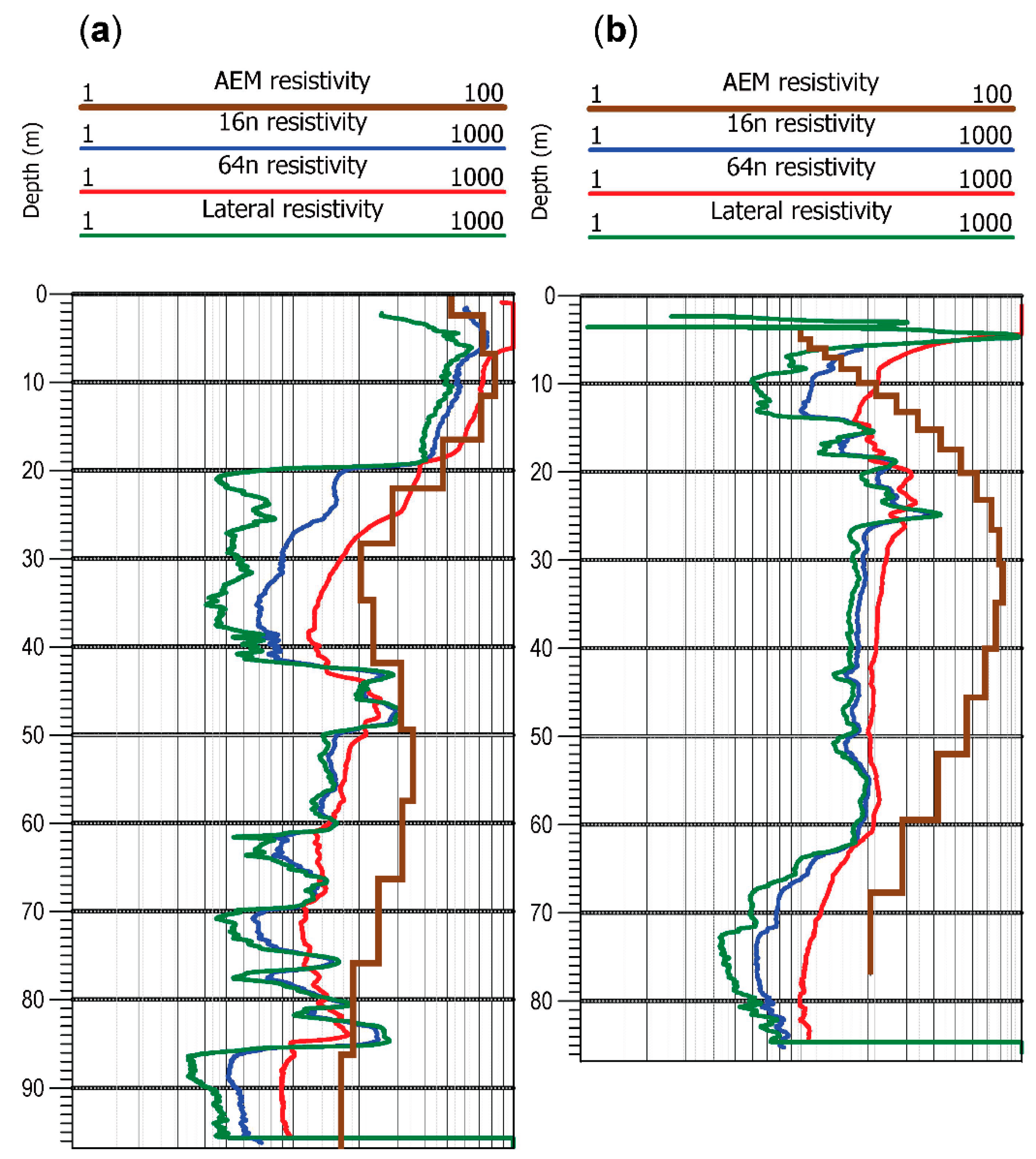
Figure 3.
Comparison of 1D inversion models of airborne electromagnetic data (brown lines) and borehole resistivity logs (colored lines) from eastern Nebraska: (a) Time domain system; (b) frequency domain system. Legends at top show ranges of resistivity values (ohm-m) along logarithmic x-axis. Brown lines are 1D vertical inversion layers from AEM. Short-normal circuit (16n) in blue, long-normal circuit (64n) in red, and lateral device in green, from conventional wireline geophysical logs of open boreholes. Note that AEM resistivity range is 1–100 ohm-m, whereas range for borehole logs is 1–1000 ohm-m.

Figure 4.
Hydrograph from observation well at Wausa (Site 1): (a) 12-year record showing drawdown and recovery during multiple irrigation seasons. Gaps are due to equipment malfunctions. Red dashed line shows gradual lowering of annual maximum water level after recovery from pumping; (b) drawdown and recovery curve from a single irrigation season (2012). Red dashed line is average linear pattern of drawdown characteristic of a bounded, compartmentalized aquifer.

Figure 5.
3D view of AEM profiles and boreholes at the Wausa site showing high-resistivity aquifer zone surrounded by conductive, impermeable clay-tills. Scale varies in this perspective. Scale bars represent distances in foreground. Field of view, left-to-right, in foreground, is approximately 2.5 km. Background is approximately 5 km.

Figure 6.
Drawdown vs. time for six observation wells at the Oakland site during a 94-h pump test. Curves in blue are from wells in upper aquifer. Curves in red are from wells in lower aquifer.
Figure 6.
Drawdown vs. time for six observation wells at the Oakland site during a 94-h pump test. Curves in blue are from wells in upper aquifer. Curves in red are from wells in lower aquifer.

Figure 7.
Geology and AEM profiles of the Oakland site: (a) Resistivity-depth profile of line 101601 without interpretations; (b) same as in a, but with interpretations. (c) geologic stack map interpreted from AEM and boreholes showing vertical successions of Quaternary stratigraphic units from the land surface to the bedrock surface. Legend shows youngest units on left and oldest units on right. Qa = alluvium; Ql = loess; Qaf2 = younger terrace alluvium; Qaf1 = older terrace alluvium; Qt = till; Qss = sub-till silt and sand; Qsg2 = younger sand and gravel; Qsg1 = older sand and gravel.

Figure 8.
Water table map of the Firth site showing extent of impermeable boundary interpreted from AEM and anomalies in contours caused by the boundary. Contour interval is 3 m.
Figure 8.
Water table map of the Firth site showing extent of impermeable boundary interpreted from AEM and anomalies in contours caused by the boundary. Contour interval is 3 m.

Figure 9.
3D view of AEM profiles and interpretation of the Firth site. Scale varies in this perspective. Scale bars represent distances in foreground.
Figure 9.
3D view of AEM profiles and interpretation of the Firth site. Scale varies in this perspective. Scale bars represent distances in foreground.

© 2018 by the author. Licensee MDPI, Basel, Switzerland. This article is an open access article distributed under the terms and conditions of the Creative Commons Attribution (CC BY) license (http://creativecommons.org/licenses/by/4.0/).
Share and Cite
MDPI and ACS Style
Korus, J. Combining Hydraulic Head Analysis with Airborne Electromagnetics to Detect and Map Impermeable Aquifer Boundaries. Water 2018, 10, 975. https://doi.org/10.3390/w10080975
AMA Style
Korus J. Combining Hydraulic Head Analysis with Airborne Electromagnetics to Detect and Map Impermeable Aquifer Boundaries. Water. 2018; 10(8):975. https://doi.org/10.3390/w10080975
Chicago/Turabian StyleKorus, Jesse. 2018. "Combining Hydraulic Head Analysis with Airborne Electromagnetics to Detect and Map Impermeable Aquifer Boundaries" Water 10, no. 8: 975. https://doi.org/10.3390/w10080975
Note that from the first issue of 2016, this journal uses article numbers instead of page numbers. See further details here.