High-Resolution Electrical Resistivity Tomography (ERT) to Characterize the Spatial Extension of Freshwater Lenses in a Salinized Coastal Aquifer

 ,
,
Abstract
:1. Introduction
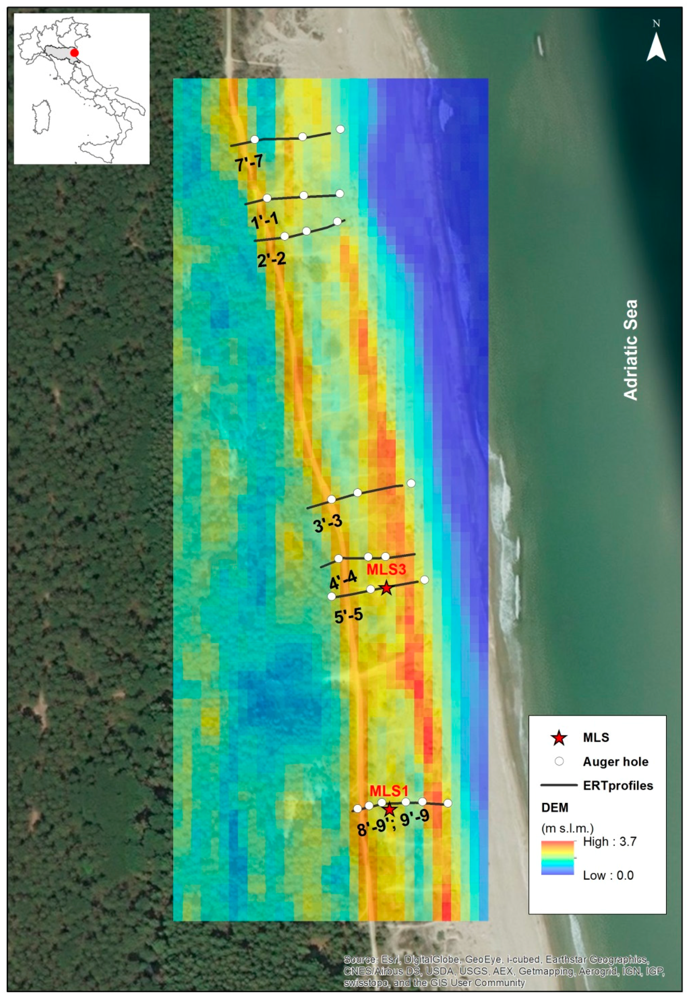
2. Study Area
Hydrogeological Setting
3. Materials and Methods
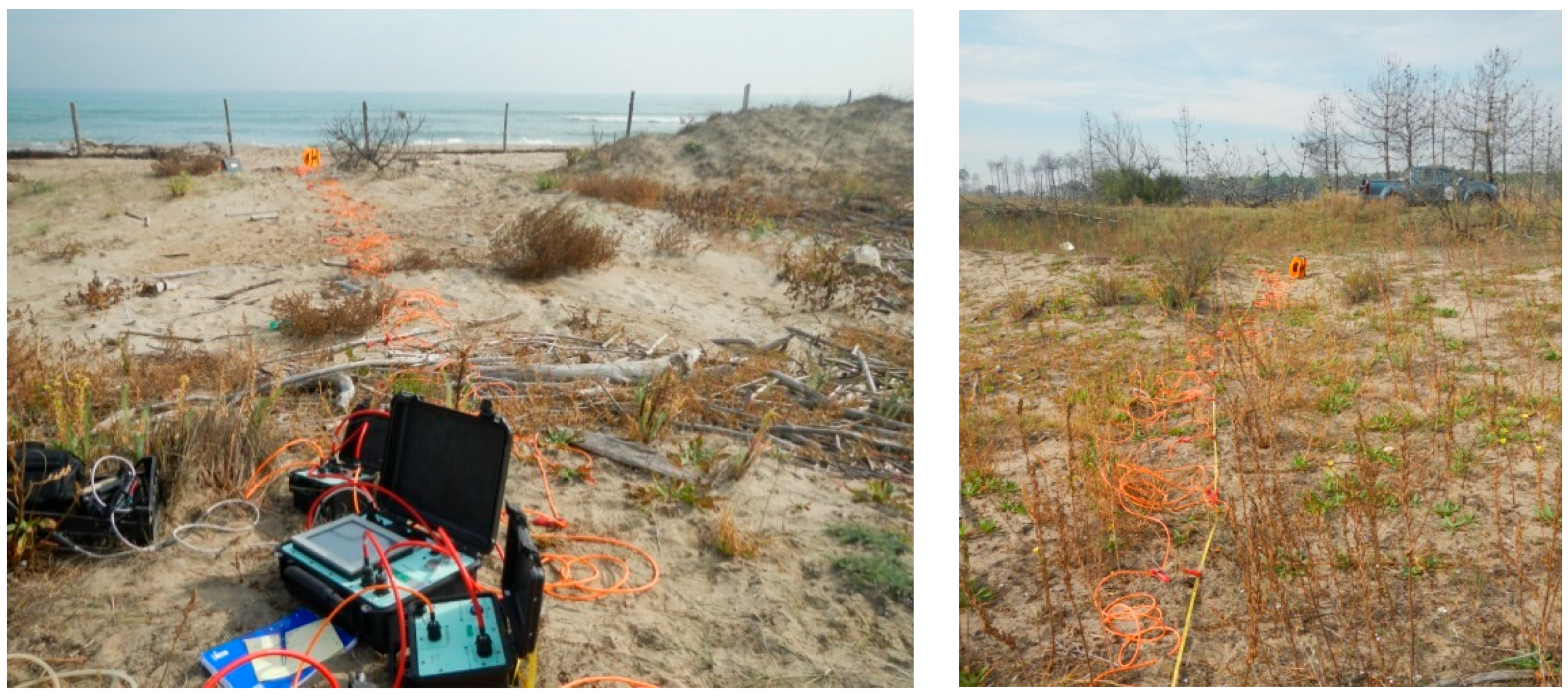
3.1. ERT Surveys
3.2. Hydrological Data
4. Results and Discussion
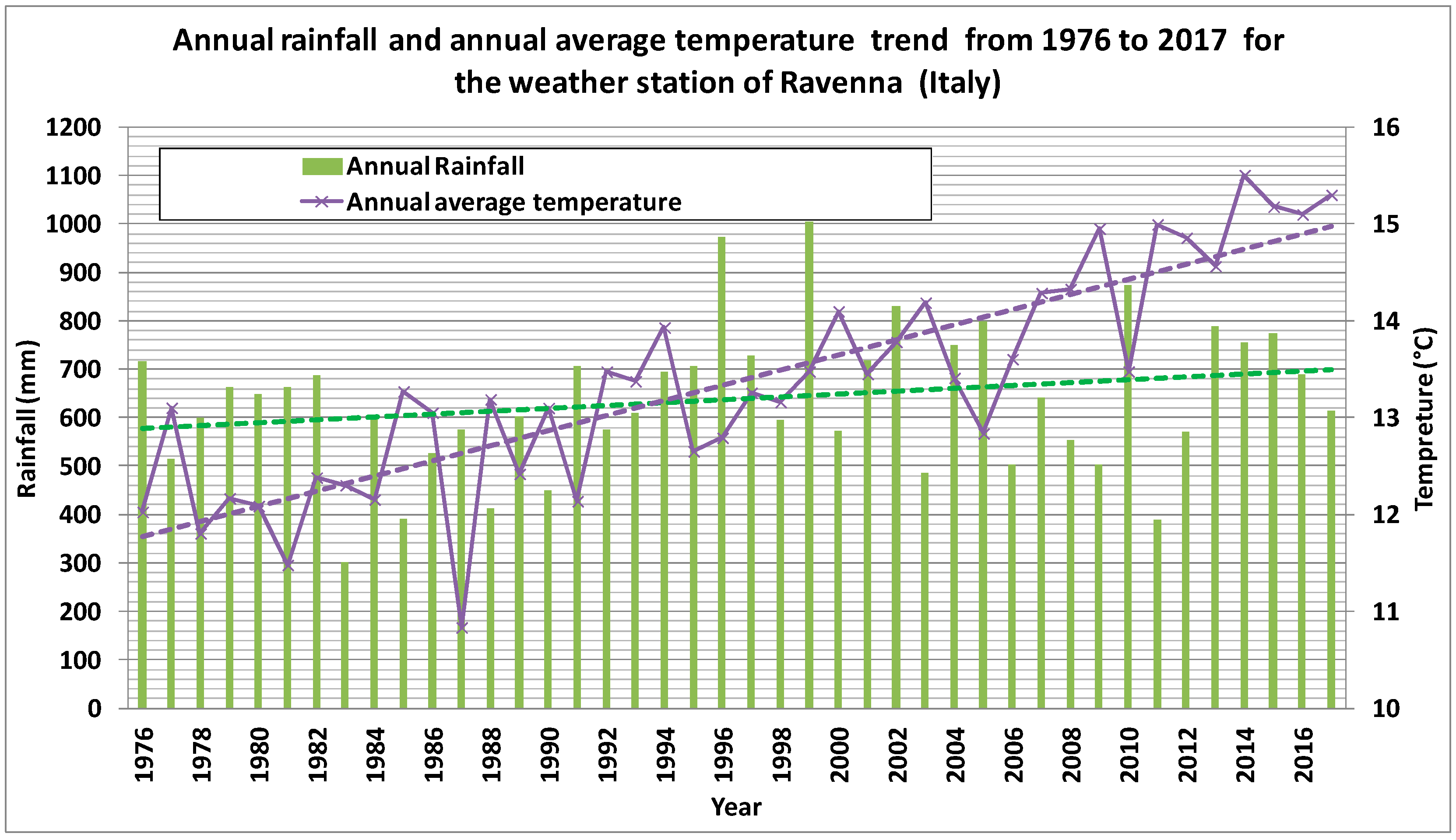
4.1. Climate Data
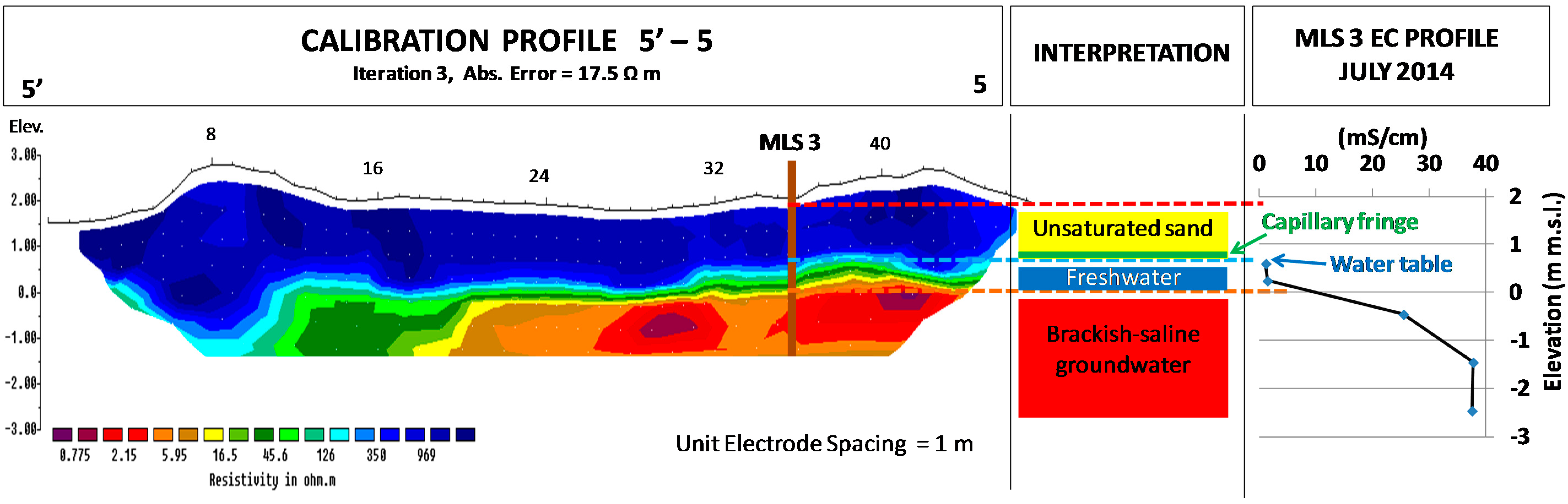
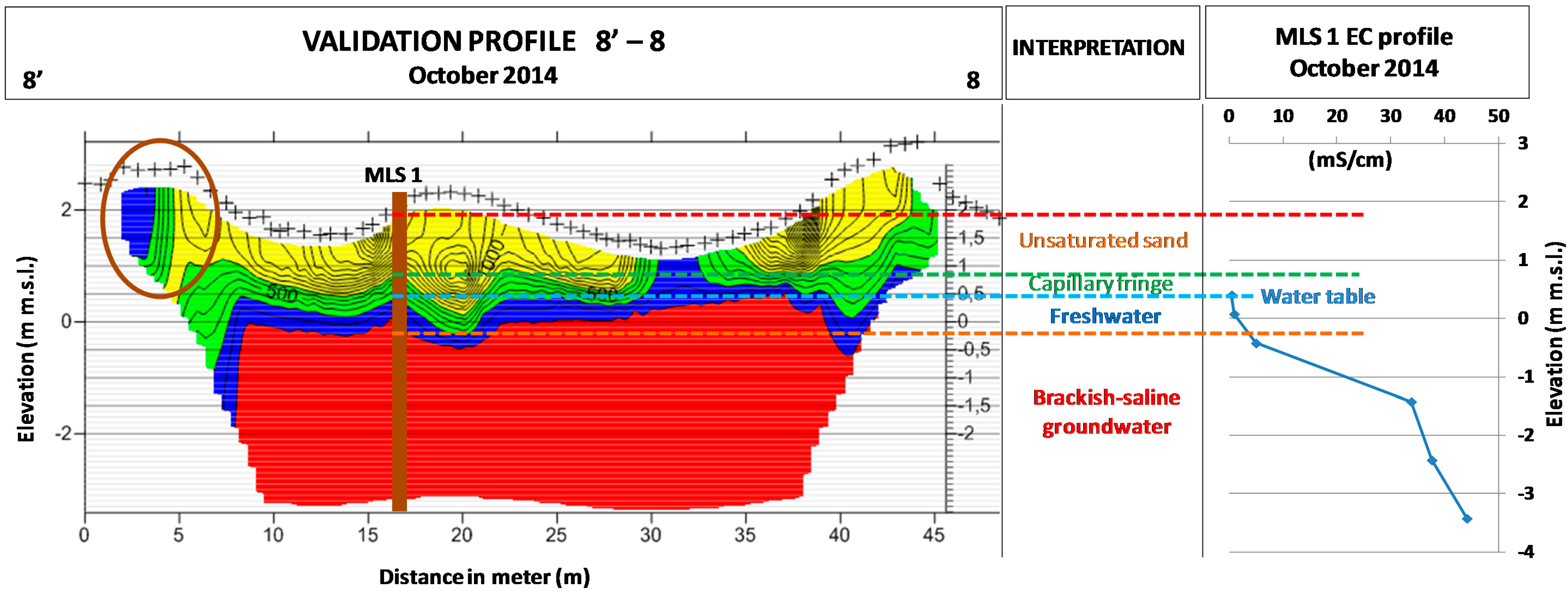
4.2. Calibration and Validation
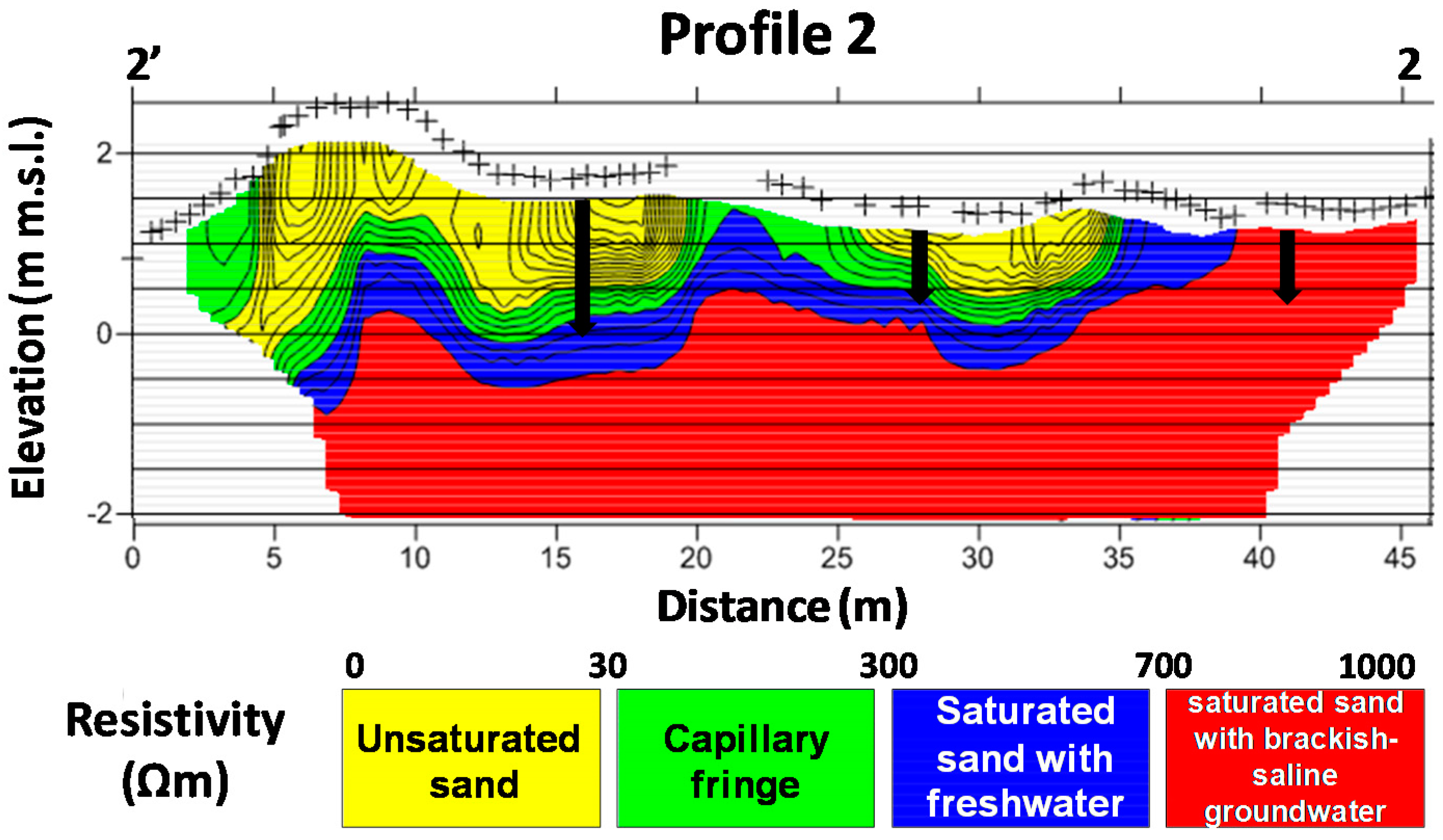
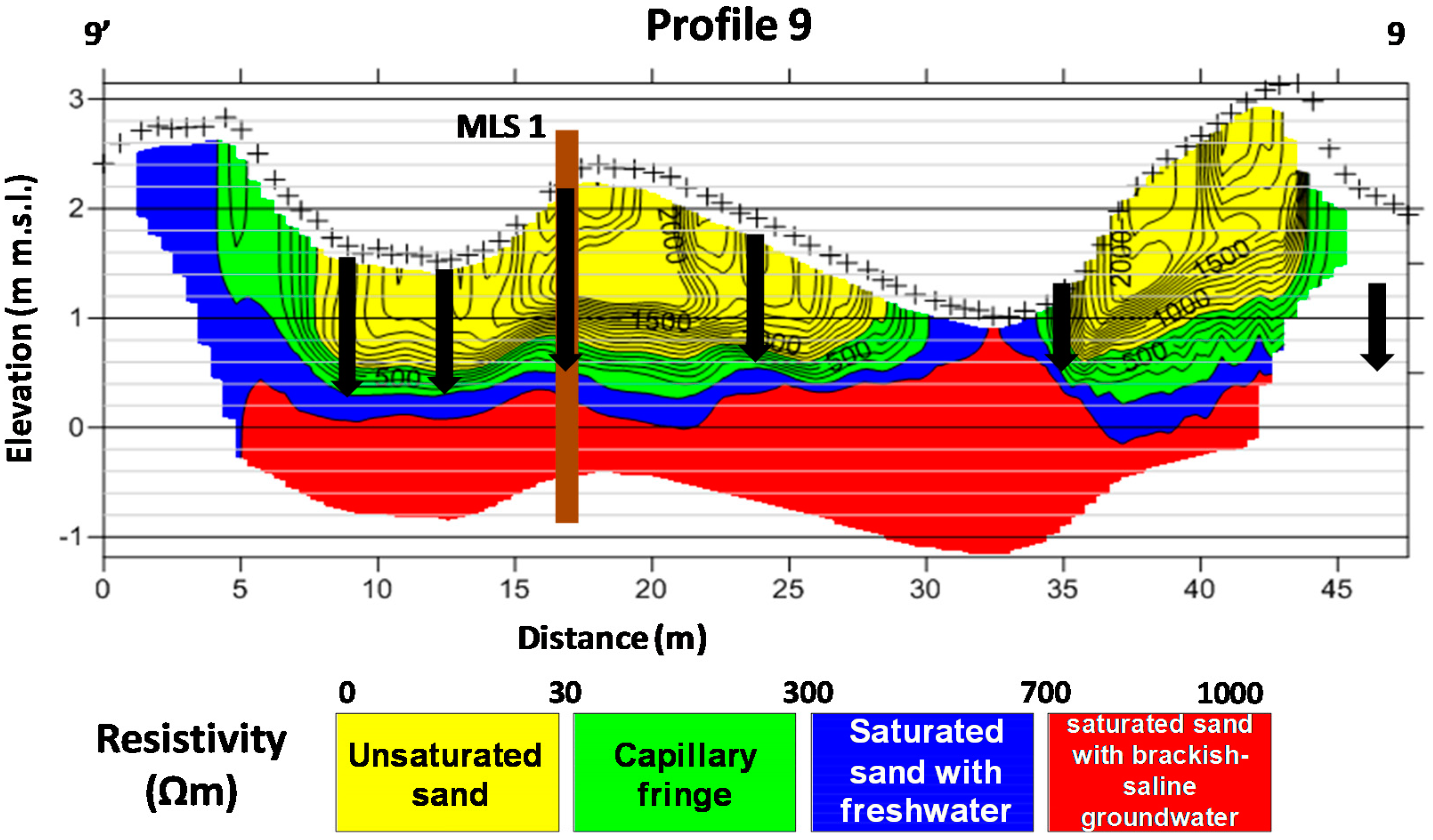
4.3. Hydrological Unit Identification
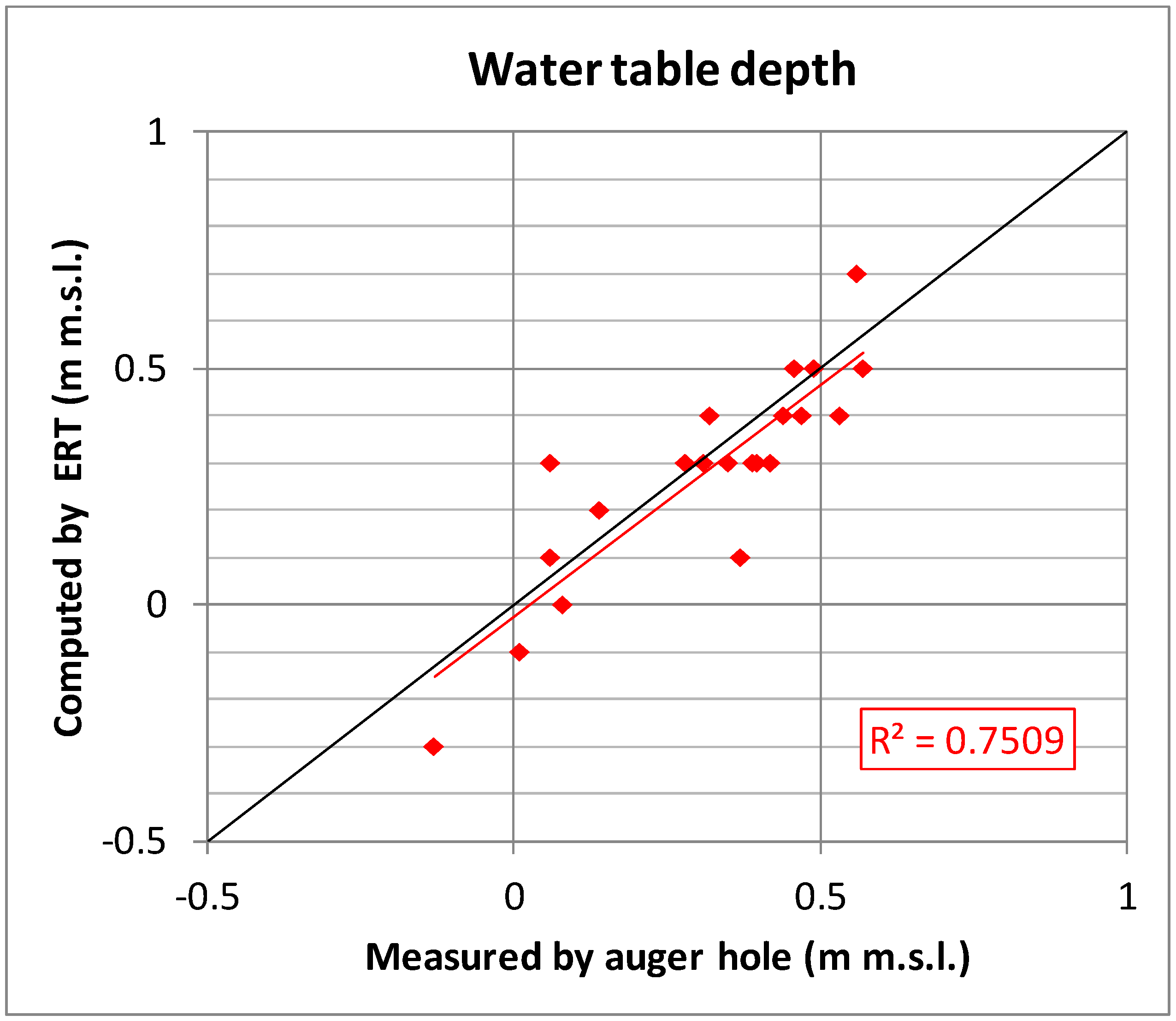
4.4. WTD
4.5. Effectiveness of the ERT
5. Conclusions
Supplementary Materials
Author Contributions
Funding
Acknowledgments
Conflicts of Interest
References
- De Louw, P.G.B.; Eeman, S.; Oude Essink, G.H.P.; Vermue, E.; Post, V.E.A. Rainwater lens dynamics and mixing between infiltrating rainwater and upward saline groundwater seepage beneath a tile-drained agricultural field. J. Hydrol. 2013, 501, 133–145. [Google Scholar] [CrossRef]
- Cellone, F.; Tosi, L.; Carol, E. Estimating the freshwater-lens reserve in the coastal plain of the middle Río de la Plata Estuary (Argentina). Sci. Total Environ. 2018, 630, 357–366. [Google Scholar] [CrossRef] [PubMed]
- Custodio, E. Aquifères côtières de l’Europe: Une vision generale. Hydrogeol. J. 2010, 18, 269–280. [Google Scholar] [CrossRef]
- Antonellini, M.; Mollema, P.N. Impact of groundwater salinity on vegetation species richness in the coastal pine forests and wetlands of Ravenna, Italy. Ecol. Eng. 2010, 36, 1201–1211. [Google Scholar] [CrossRef]
- Drabbe, J.; Ghijben, B.W. Nota in verband met de voorgenomen putboring nabij Amsterdam. Van Konink. Inst. Van Ing. 1889, 5, 8–22. [Google Scholar]
- Herzberg, A. Die wasserversorgung einiger Nordseebader. J. Gasbeleucht. Wasserversorg. 1901, 44, 842–844. [Google Scholar]
- De Louw, P.G.B.; Eeman, S.; Siemon, B.; Voortman, B.R.; Gunnink, J.; Van Baaren, E.S.; Oude Essink, G.H.P. Shallow rainwater lenses in deltaic areas with saline seepage. Hydrol. Earth Syst. Sci. 2011, 15, 3659–3678. [Google Scholar] [CrossRef] [Green Version]
- Pinna, M.S.; Cogoni, D.; Fenu, G.; Bacchetta, G. The conservation status and anthropogenic impacts assessments of Mediterranean coastal dunes. Estuar. Coast. Shelf Sci. 2015, 167, 25–31. [Google Scholar] [CrossRef]
- Olson, J.S. Lake Michigan dune development 2. Plants as agents and tools in geomorphology. J. Geol. 1958, 66, 345–351. [Google Scholar] [CrossRef]
- Eeman, S.; Leijnse, A.; Raats, P.A.C.; van der Zee, S.E.A.T.M. Analysis of the thickness of a fresh water lens and of the transition zone between this lens and upwelling saline water. Adv. Water Resour. 2011, 34, 291–302. [Google Scholar] [CrossRef]
- Zarroca, M.; Bach, J.; Linares, R.; Pellicer, X.M. Electrical methods (VES and ERT) for identifying, mapping and monitoring different saline domains in a coastal plain region (Alt Empordà, Northern Spain). J. Hydrol. 2011, 409, 407–422. [Google Scholar] [CrossRef]
- Tajul Baharuddin, M.F.; Othman, A.R.; Taib, S.; Hashim, R.; Zainal Abidin, M.H.; Radzuan, M.A. Evaluating freshwater lens morphology affected by seawater intrusion using chemistry-resistivity integrated technique: A case study of two different land covers in Carey Island, Malaysia. Environ. Earth Sci. 2013, 69, 2779–2797. [Google Scholar] [CrossRef] [Green Version]
- Cozzolino, D.; Greggio, N.; Antonellini, M.; Giambastiani, B.M.S. Natural and anthropogenic factors affecting freshwater lenses in coastal dunes of the Adriatic coast. J. Hydrol. 2017, 551, 804–818. [Google Scholar] [CrossRef]
- Oude Essink, G.H.P.; van Baaren, E.S.; de Louw, P.G.B. Effects of climate change on coastal groundwater systems: A modeling study in The Netherlands. Water Resour. Res. 2010, 46, 1–16. [Google Scholar] [CrossRef]
- Balugani, E.; Antonellini, M. Measuring salinity within shallow piezometers: Comparison of two field methods. J. Water Resour. Prot. 2010, 2, 251. [Google Scholar] [CrossRef]
- Land, L.A.; Lautier, J.C.; Wilson, N.C.; Chianese, G.; Webb, S. Geophysical Monitoring and Evaluation of Coastal Plain Aquifers. Ground Water 2004, 42, 59–67. [Google Scholar] [CrossRef] [PubMed]
- Rey, J.; Martínez, J.; Barberá, G.G.; García-Aróstegui, J.L.; García-Pintado, J.; Martínez-Vicente, D. Geophysical characterization of the complex dynamics of groundwater and seawater exchange in a highly stressed aquifer system linked to a coastal lagoon (SE Spain). Environ. Earth Sci. 2013, 70, 2271–2282. [Google Scholar] [CrossRef]
- Francés, A.P.; Ramalho, E.C.; Fernandes, J.; Groen, M.; Hugman, R.; Khalil, M.A.; De Plaen, J.; Monteiro Santos, F.A. Contributions de l’hydrogéophysique au modèle conceptuel hydrogéologique de l’aquifère côtier Albufeira-Riberia de Quarteira en Algarve, Portugal. Hydrogeol. J. 2015, 23, 1553–1572. [Google Scholar] [CrossRef]
- Kazakis, N.; Pavlou, A.; Vargemezis, G.; Voudouris, K.S.; Soulios, G.; Pliakas, F.; Tsokas, G. Seawater intrusion mapping using electrical resistivity tomography and hydrochemical data. An application in the coastal area of eastern Thermaikos Gulf, Greece. Sci. Total Environ. 2016, 543, 373–387. [Google Scholar] [CrossRef] [PubMed]
- García-menéndez, O.; Ballesteros, B.J.; Renau-Pruñonosa, A.; Morell, I.; Mochales, T.; Ibarra, P.I.; Rubio, F.M. Using electrical resistivity tomography to assess the effectiveness of managed aquifer recharge in a salinized coastal aquifer. Environ. Monit. Assess. 2018, 190, 100. [Google Scholar] [CrossRef] [PubMed]
- Kumar, K.S.A.; Priju, C.P.; Prasad, N.B.N. Study on Saline Water Intrusion into the Shallow Coastal Aquifers of Periyar River Basin, Kerala Using Hydrochemical and Electrical Resistivity Methods. Aquat. Procedia 2015, 4, 32–40. [Google Scholar] [CrossRef]
- Galazoulas, E.C.; Mertzanides, Y.C.; Petalas, C.P.; Kargiotis, E.K. Large Scale Electrical Resistivity Tomography Survey Correlated to Hydrogeological Data for Mapping Groundwater Salinization: A Case Study from a Multilayered Coastal Aquifer in Rhodope, Northeastern Greece. Environ. Process. 2015, 2, 19–35. [Google Scholar] [CrossRef] [Green Version]
- Kirsch, R.; Yaramanci, U. Geoelectrical methods. In Groundwater Geophysics: A Tool for Hydrogeology; Kirsch, R., Ed.; Springer: Berlin/Heidelberg, Germany, 2009; pp. 85–117. ISBN 978-3-540-88405-7. [Google Scholar]
- Wilkinson, P.B.; Meldrum, P.I.; Kuras, O.; Chambers, J.E.; Holyoake, S.J.; Ogilvy, R.D. High-resolution Electrical Resistivity Tomography monitoring of a tracer test in a confined aquifer. J. Appl. Geophys. 2010, 70, 268–276. [Google Scholar] [CrossRef] [Green Version]
- European Parliament. Directive 2009/147/EC of the European Parliament and of the Council of 30 November 2009 on the conservation of wild birds. Off. J. Eur. Union 2010, 32, 128–146. [Google Scholar]
- The Council of the European Communities. Council Directive 92/43/EEC of 21 May 1992 on the conservation of natural habitats and of wild fauna and flora. Off. J. 1992, L 206, 7–50. [Google Scholar]
- United Nations Educational, Scientific and Cultural Organization. The convention on wetlands of international importance especially as waterfowl habitat. Environ. Policy Law 1983, 996, 245. [Google Scholar] [CrossRef]
- Teatini, P.; Ferronato, M.; Gambolati, G.; Bertoni, W.; Gonella, M. A century of land subsidence in Ravenna, Italy. Environ. Geol. 2005, 47, 831–846. [Google Scholar] [CrossRef]
- Taramelli, A.; Di Matteo, L.; Ciavola, P.; Guadagnano, F.; Tolomei, C. Temporal evolution of patterns and processes related to subsidence of the coastal area surrounding the Bevano River mouth (Northern Adriatic)—Italy. Ocean Coast. Manag. 2015, 108, 74–88. [Google Scholar] [CrossRef]
- Sytnik, O.; Stecchi, F. Disappearing coastal dunes: Tourism development and future challenges, a case-study from Ravenna, Italy. J. Coast. Conserv. 2015, 19, 715–727. [Google Scholar] [CrossRef]
- Ciavola, P.; Armaroli, C.; Chiggiato, J.; Valentini, A.; Deserti, M.; Perini, L.; Luciani, P. Impact of storms along the coastline of Emilia-Romagna: The morphological signature on the Ravenna coastline (Italy). J. Coast. Res. 2007, 50, 1–5. [Google Scholar]
- Giambastiani, B.M.S.; Colombani, N.; Greggio, N.; Antonellini, M.; Mastrocicco, M. Coastal aquifer response to extreme storm events in Emilia-Romagna, Italy. Hydrol. Process. 2017, 31, 1613–1621. [Google Scholar] [CrossRef]
- Giambastiani, B.M.S.; Greggio, N.; Nobili, G.; Dinelli, E.; Antonellini, M. Forest fire effects on groundwater in a coastal aquifer (Ravenna, Italy). Hydrol. Process. 2018, 32, 2377–2389. [Google Scholar] [CrossRef]
- Amorosi, A.; Colalongo, M.L.; Fiorini, F.; Fusco, F.; Pasini, G.; Vaiani, S.C.; Sarti, G. Palaeogeographic and palaeoclimatic evolution of the Po Plain from 150-ky core records. Glob. Planet. Chang. 2004, 40, 55–78. [Google Scholar] [CrossRef]
- Amorosi, A.; Colalongo, M.L.; Pasini, G.; Preti, D. Sedimentary response to Late Quaternary sea-level changes in the Romagna coastal plain (northern Italy). Sedimentology 1999, 46, 99–121. [Google Scholar] [CrossRef]
- Francés, A.P.; Su, Z.; Lubczynski, M.W. Integration of Hydrogeophysics and Remote Sensing with Coupled Hydrological Models. Ph.D. Thesis, University of Twente, Enschede, The Netherlands, 17 July 2015. [Google Scholar]
- Warner, D.L. Preliminary field studies using earth resistivity measurements for delineating zones of contaminated ground water. Groundwater 1969, 7, 9–16. [Google Scholar] [CrossRef]
- Geotomo Software. RES2DINV ver. 3.59 for Windows XP/Vista/7. Rapid 2-D resistivity and IP inversion using the least-squares method. In Geoelectrical Imaging 2D & 3D; Geotomo Software: Penang, Malaysia, 2010. [Google Scholar]
- DeGroot-Hedlin, C.; Constable, S. Occam’s inversion to generate smooth, two-dimensional models from magnetotelluric data. Geophysics 1990, 55, 1613–1624. [Google Scholar] [CrossRef]
- Batayneh, A.T. Use of electrical resistivity methods for detecting subsurface fresh and saline water and delineating their interfacial configuration: A case study of the eastern Dead Sea coastal aquifers, Jordan. Hydrogeol. J. 2006, 14, 1277–1283. [Google Scholar] [CrossRef]
- Bauer, P.; Supper, R.; Zimmermann, S.; Kinzelbach, W. Geoelectrical imaging of groundwater salinization in the Okavango Delta, Botswana. J. Appl. Geophys. 2006, 60, 126–141. [Google Scholar] [CrossRef]
- Sherif, M.; El Mahmoudi, A.; Garamoon, H.; Kacimov, A.; Akram, S.; Ebraheem, A.; Shetty, A. Geoelectrical and hydrogeochemical studies for delineating seawater intrusion in the outlet of Wadi Ham, UAE. Environ. Geol. 2006, 49, 536–551. [Google Scholar] [CrossRef]
- Post, V.; Kooi, H.; Simmons, C. Using hydraulic head measurements in variable-density ground water flow analyses. Ground Water 2007, 45, 664–671. [Google Scholar] [CrossRef] [PubMed]
- ARPAE Luglio 2014: Analisi di un’anomalia Meteorologica. Available online: https://www.arpae.it/dettaglio_notizia.asp?id=5757&idlivello=962 (accessed on 26 July 2018).
- Sabia, M.; Antonellini, M.; Gabbianelli, G.; Giambastiani, B.; Lapenna, V.; Perrone, A.; Rizzo, E. Indagini geoelettriche per lo studio di strutture idrogeologiche nella Pineta di San Vitale (RA) [Geo-resistivity investigations for the characterization of hydrogeologic structures in the San Vitale Pine Forest (RA)]. In Proceedings of the Acta National Geophysical Meeting Solid Earth, Rome, Italy, 15–17 November 2005. [Google Scholar]
- Giambastiani, B.M.S.; Antonellini, M.; Essink, G.H.P.O.; Stuurman, R.J. Saltwater intrusion in the unconfined coastal aquifer of Ravenna (Italy): A numerical model. J. Hydrol. 2007, 340, 91–104. [Google Scholar] [CrossRef]
- Antonellini, M.; Mollema, P.; Giambastiani, B.; Bishop, K.; Caruso, L.; Minchio, A.; Pellegrini, L.; Sabia, M.; Ulazzi, E.; Gabbianelli, G. Salt water intrusion in the coastal aquifer of the southern Po Plain, Italy. Hydrogeol. J. 2008, 16, 1541. [Google Scholar] [CrossRef]
- Mollema, P.N.; Antonellini, M.; Dinelli, E.; Gabbianelli, G.; Greggio, N.; Stuyfzand, P.J. Hydrochemical and physical processes influencing salinization and freshening in Mediterranean low-lying coastal environments. Appl. Geochem. 2013, 34, 207–221. [Google Scholar] [CrossRef]
- Vandenbohede, A.; Mollema, P.N.; Greggio, N.; Antonellini, M. Seasonal dynamic of a shallow freshwater lens due to irrigation in the coastal plain of Ravenna, Italy. Hydrogeol. J. 2014, 22, 893–909. [Google Scholar] [CrossRef]
- Morgan, L.K.; Werner, A.D. Seawater intrusion vulnerability indicators for freshwater lenses in strip islands. J. Hydrol. 2014, 508, 322–327. [Google Scholar] [CrossRef]
- Tanjal, C.; Carol, E.; Richiano, S.; Santucci, L. Freshwater lenses as ecological and population sustenance, case study in the coastal wetland of Samborombón Bay (Argentina). Mar. Pollut. Bull. 2017, 122, 426–431. [Google Scholar] [CrossRef] [PubMed]
- Samouëlian, A.; Cousin, I.; Tabbagh, A.; Bruand, A.; Richard, G. Electrical resistivity survey in soil science: A review. Soil Tillage Res. 2005, 83, 173–193. [Google Scholar] [CrossRef] [Green Version]
- Antonellini, M.; Allen, D.M.; Mollema, P.N.; Capo, D.; Greggio, N. Groundwater freshening following coastal progradation and land reclamation of the Po Plain, Italy. Hydrogeol. J. 2015, 23, 1009–1026. [Google Scholar] [CrossRef]
- Negri, S.; Leucci, G.; Mazzone, F. High resolution 3D ERT to help GPR data interpretation for researching archaeological items in a geologically complex subsurface. J. Appl. Geophys. 2008, 65, 111–120. [Google Scholar] [CrossRef]


| >700 Ωm | Unsaturated sand | Unsaturated zone |
| 700–300 Ωm | Capillary fringe | |
| 300–30 Ωm | Freshwater | Saturated zone |
| <30 Ωm | Brackish-saline groundwater |
| Profile | Auger Hole | EC (mS/cm) | WTD (m m.s.l.) | |||
|---|---|---|---|---|---|---|
| Auger Hole | Computed ERT | Auger Hole | Computed ERT | |||
| 7 | sea | 35.5 | Salty | Out of the ERT domain | 0.21 | Out of the ERT domain |
| 7 | middle | 13.9 | Salty | Fresh | 0.44 | 0.4 |
| 7 | inland | 6.5 | Salty | Salty | 0.49 | 0.5 |
| 1 | sea | 36.2 | Salty | Salty | 0.3 | Bordering the ERT domain |
| 1 | middle | 17.7 | Salty | Fresh | 0.47 | 0.4 |
| 1 | inland | 4.5 | Salty | Fresh | 0.14 | 0.2 |
| 2 | sea | 31.1 | Salty | Salty | 0.31 | Bordering the ERT domain |
| 2 | middle | 3.8 | Fresh | Fresh | 0.39 | 0.3 |
| 2 | inland | 2.4 | Fresh | Fresh | 0.01 | −0.1 |
| 3 | sea | 9.3 | Salty | Out of the ERT domain | −0.05 | Out of the ERT domain |
| 3 | middle | 0.6 | Fresh | Fresh | 0.35 | 0.3 |
| 3 | inland | 0.9 | Fresh | Fresh | 0.06 | 0.3 |
| 4 | sea | 7.6 | Salty | Fresh | −0.13 | −0.3 |
| 4 | middle | 11.7 | Salty | Fresh | 0.37 | 0.1 |
| 4 | inland | 0.8 | Fresh | Fresh | 0.08 | 0.0 |
| 5 | sea | 10.3 | Salty | Out of the ERT domain | 0.07 | Out of the ERT domain |
| 5 | middle | 0.4 | Fresh | Fresh | 0.28 | 0.3 |
| 5 | inland | 0.7 | Fresh | Fresh | 0.06 | 0.1 |
| 8 | sea | 0.6 | Fresh | Fresh | 0.56 | 0.7 |
| 8 | middle | 0.3 | Fresh | Fresh | 0.32 | 0.4 |
| 8 | inland | 0.3 | Fresh | Fresh | 0.31 | 0.3 |
| 9 | sea | 6.8 | Salty | Out of the ERT domain | 0.516 | Out of the ERT domain |
| 9 | middle | 0.5 | Fresh | Fresh | 0.532 | 0.4 |
| 9 | middle | 0.5 | Fresh | Fresh | 0.458 | 0.5 |
| 9 | middle | 0.6 | Fresh | Fresh | 0.57 | 0.5 |
| 9 | middle | 0.4 | Fresh | Fresh | 0.419 | 0.3 |
| 9 | inland | 0.5 | Fresh | Fresh | 0.397 | 0.3 |
© 2018 by the authors. Licensee MDPI, Basel, Switzerland. This article is an open access article distributed under the terms and conditions of the Creative Commons Attribution (CC BY) license (http://creativecommons.org/licenses/by/4.0/).
Share and Cite
Greggio, N.; Giambastiani, B.M.S.; Balugani, E.; Amaini, C.; Antonellini, M. High-Resolution Electrical Resistivity Tomography (ERT) to Characterize the Spatial Extension of Freshwater Lenses in a Salinized Coastal Aquifer. Water 2018, 10, 1067. https://doi.org/10.3390/w10081067
Greggio N, Giambastiani BMS, Balugani E, Amaini C, Antonellini M. High-Resolution Electrical Resistivity Tomography (ERT) to Characterize the Spatial Extension of Freshwater Lenses in a Salinized Coastal Aquifer. Water. 2018; 10(8):1067. https://doi.org/10.3390/w10081067
Chicago/Turabian StyleGreggio, Nicolas, Beatrice M. S. Giambastiani, Enrico Balugani, Chiara Amaini, and Marco Antonellini. 2018. "High-Resolution Electrical Resistivity Tomography (ERT) to Characterize the Spatial Extension of Freshwater Lenses in a Salinized Coastal Aquifer" Water 10, no. 8: 1067. https://doi.org/10.3390/w10081067