Article

Comparing Bias Correction Methods Used in Downscaling Precipitation and Temperature from Regional Climate Models: A Case Study from the Kaidu River Basin in Western China

1
State Key Laboratory of Desert and Oasis Ecology, Xinjiang Institute of Ecology and Geography, Chinese Academy of Sciences, Urumqi 830011, China
2
Department of Geography, Ghent University, 9000 Gent, Belgium
3
University of Chinese Academy of Science, Beijing 100039, China
4
Sino-Belgian Joint Laboratory of Geo-Information, Urumqi 830011, China
5
Sino-Belgian Joint Laboratory of Geo-Information, 9000 Gent, Belgium
6
Research Fund Flanders (FWO), 1000 Brussels, Belgium
*
Author to whom correspondence should be addressed.
Water 2018, 10(8), 1046; https://doi.org/10.3390/w10081046
Submission received: 29 May 2018 / Revised: 29 July 2018 / Accepted: 1 August 2018 / Published: 7 August 2018
(This article belongs to the Section Hydrology)

Abstract

:
The systemic biases of Regional Climate Models (RCMs) impede their application in regional hydrological climate-change effects analysis and lead to errors. As a consequence, bias correction has become a necessary prerequisite for the study of climate change. This paper compares the performance of available bias correction methods that focus on the performance of precipitation and temperature projections. The hydrological effects of these correction methods are evaluated by the modelled discharges of the Kaidu River Basin. The results show that all used methods improve the performance of the original RCM precipitation and temperature simulations across a number of levels. The corrected results obtained by precipitation correction methods demonstrate larger diversities than those produced by the temperature correction methods. The performance of hydrological modelling is highly influenced by the choice of precipitation correction methods. Furthermore, no substantial differences can be identified from the results of the temperature-corrected methods. The biases from input data are often greater from the works of hydrological modelling. The suitability of these approaches depends upon the regional context and the RCM model, while their application procedure and a number of results can be adapted from region to region.

1. Introduction

The Intergovernmental Panel on Climate Change (IPCC) has observed that climate variable changes associated with global warming are affecting regional or catchment scale hydrological processes [1]. Changes in precipitation and temperature are anticipated as direct driving factors because they are the main factors that influence regional hydrological processes [2]. The Regional Climate Models (RCMs) provide a new opportunity for climate change effects analysis since they have a higher spatial resolution and more reliable results on a regional scale compared to General Circulation Models (GCMs) [3,4,5]. Numerous studies have shown that RCM outputs improve the representation of climate change information at the mesoscale by providing spatially and physically coherent outputs with observations [4,5]. However, the original RCM outputs still contain considerable bias, which is inherited from the forcing of GCMs or produced by systematic model error [6,7]. Furthermore, such biases may be amplified when climate change effects are included, such as in hydrological effect studies [4]. Therefore, bias correction of RCM data is the prerequisite step to the data being used in any climate change effects analysis.
Many bias correction methods, ranging from simple scaling techniques to the rather more sophisticated distribution mapping techniques, have been developed to correct biased RCM outputs [8]. The scaling approach mainly includes linear or nonlinear approaches that adjust the climatic factors based on the differences between observed and RCM means in a linear or nonlinear formula, such as the linear scaling method (LS) [9,10] and the power transpiration method (PT) [11]. Distribution mapping, involving distribution-based and distribution-free quantile mapping methods, matches the statistical distribution of RCM-simulated climatic factors to the distribution of observations. Distribution-based quantile mapping is based on the assumption that climatic factors obey a certain distribution, such as Gamma and Gaussian distributions [4,12], while the distribution-free quantile mapping technique employs the empirical distribution [13]. Selecting a suitable bias correction method is important for providing reliable inputs for impact analysis of a region.
Teutschbein and Seibert [8] applied six ensemble statistical and bias correction methods to correct precipitation and temperature data from eleven different RCM outputs in five typical catchments in Sweden. The results suggest that most methods were able to correct daily mean values to a certain extent, while only higher-skill approaches, such as distribution mapping and power transformation methods, performed well in hydrological extremes. Chen, Brissette, Chaumont and Braun [4] investigated the performance and uncertainty of two change factor and four bias correction methods in quantifying the climate change effects over Manicouagan 5 and Chickasawhay basins. It indicated that the uncertainties that result from RCM simulations are slightly greater than those from different bias correction methods. Chen, Brissette, Chaumont and Braun [13] compared the performances of six bias correction methods in four RCM-simulated precipitation events over ten North American river basins. The results demonstrate that all bias correction methods are capable of reducing bias in raw RCM, while performances of hydrological modelling are highly dependent on the locations of the catchments and the choice of bias correction methods. Setting these recent studies aside, contributions that compare and evaluate different kinds of bias correction methods in hydrological modelling are still rare in the literature, in particular over arid mountainous areas. Moreover, only a few have provided the best combination of bias correction methods for precipitation and temperature over a specific region.
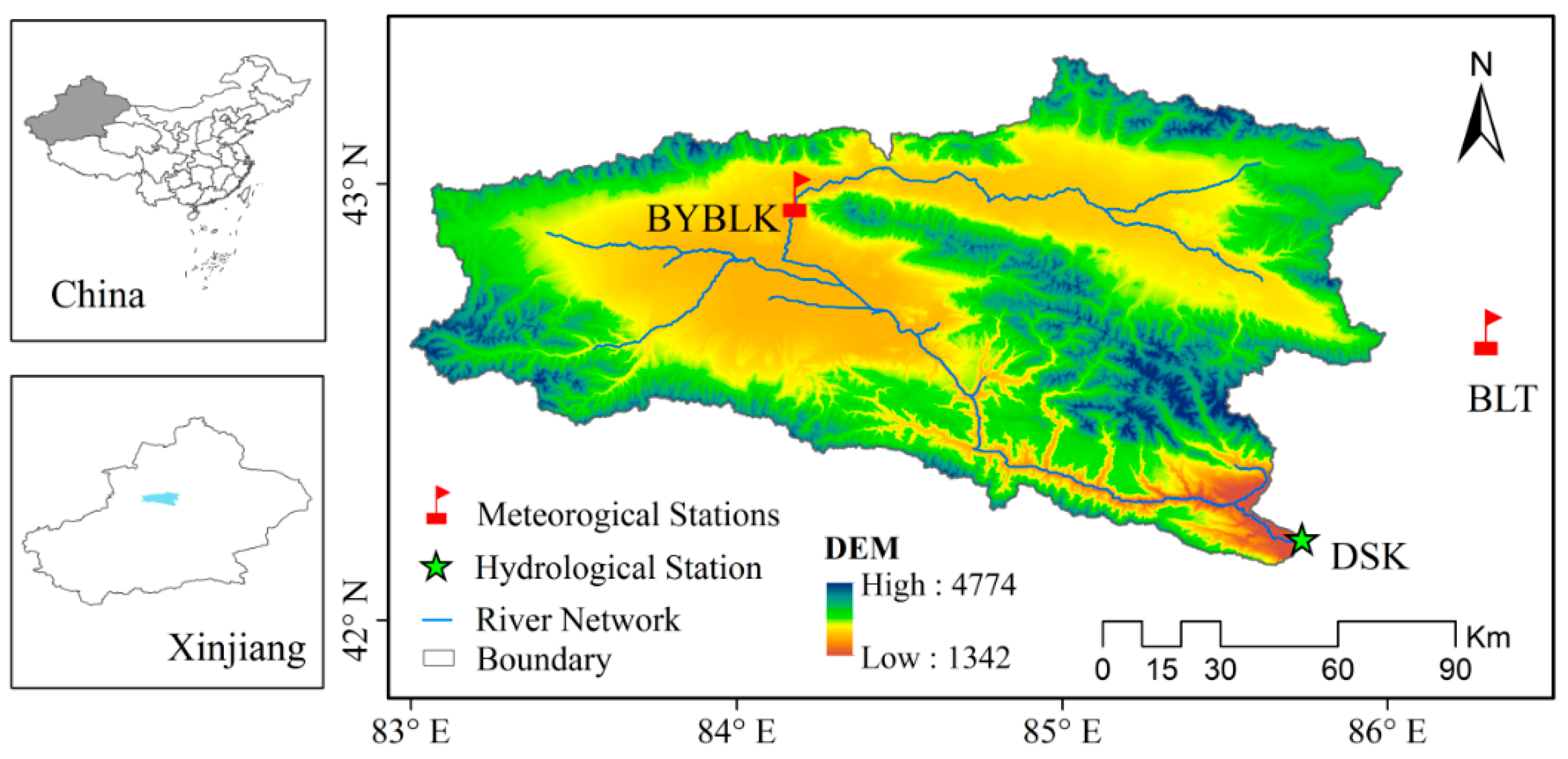
Xinjiang Uygur Autonomous Region, which is an arid and semi-arid region and located in Central Asia, is extremely vulnerable to climate change effects, since most water sources originate from the upper mountainous regions [14,15]. It is necessary to select suitable bias correction methods for providing credible inputs to estimate climate change effects over the region. Therefore, the Kaidu River Basin, one of the typical mountainous catchments in Xinjiang, was selected as a case study. The objective of the present study is to investigate the performance of available bias correction methods for downscaling climatic outputs of RCM and provide the best combination of bias correction methods for precipitation and temperature over an arid mountainous region. This paper compares existing bias correction methods of climate and hydrological projections. Seven precipitation correction methods and five temperature correction methods cover most of the existing bias correction methods that are included with the intention of correcting deviations in this study. The influence of bias correction methods on hydrological simulations is studied by comparing different discharge outputs. This is achieved by using SWAT hydrological modelling with original RCM data and all possible combinations of corrected precipitation and temperature data.

2. Study Area and Data

2.1. Study Area

The Kaidu River Basin is situated on the southern slope of Tianshan Mountains, Xinjiang, China. It is enclosed between a longitude of 82°58′–86°05′ E and a latitude of 42°14′–43°21′ N [16], and covers an area of ca. 18,827 km2 (Figure 1). This region has a complex topography, including grassland, marshland, surrounding mountainous alpine areas, and woodland [15,17]. Its elevation extends from 1342 m to 4774 m, with an average elevation of 2995 m above sea level (asl) [18]. Meteorological parameters covering the period of 1965–2005 from the China Meteorological Data Sharing Service System (http://data.cma.cn/) suggest that the average annual precipitation is ca. 294 mm and the annual average temperature is −3.8 °C at the Bayinbuluke (BYBLK) meteorological station (Figure 2). The annual maximum and minimum temperatures are 18.8 °C and −44.6 °C, respectively. The measured total annual pan evaporation exceeds 1017 mm [16].
Precipitation which takes the form of snowfall lasts from November to March and is stored as a solid form. The total number of snow cover days is ca. 139.3 days and the average snow depth is 120 mm [19,20]. Water resources in the headwater region mainly originate from season snowmelt in spring, while during the summer months, they are provided by a mixture of melting glaciers and rainfall [21]. Figure 2 demonstrates that there are two main flood peaks throughout the whole year: the first one arises from seasonal snowmelt during April and the latter is mainly attributable to precipitation during the months of July and August. The mean annual discharge at the Dashankou (DSK) hydrological station is ca. 35.03 × 10⁸ m3 with a runoff depth of ca. 143.2 mm.

2.2. Data

The daily observed meteorological data, including precipitation and average/maximum/minimum temperatures from the BYBLK and Baluntai (BLT) stations (Figure 1), provide the reference material that is used to correct RCM outputs. They are taken from the China Meteorological Data Sharing Service System (http://data.cma.cn/). The observed discharges at the DSK station are provided by the Tarim Water Resources Management Bureau. RCM outputs from HadGEM3-RA, with a horizontal resolution of ca. 50 km for the 1965–2004 period, are used in this study. The HadGEM3-RA model is taken from the Coordinated Regional Climate Downscaling Experiment (CORDEX) for East Asia [22]. The nearest neighbour method is adopted to extract the grid points at site locations with the intention of comparing the observations with RCM model outputs. To set up the SWAT model, spatial datasets covering the topographic data, land cover data, and soil property data are also needed. The digital elevation data (DEM) at a 90 m spatial resolution from the NASA Shuttle Radar Topographic Mission (SRTM) was used in our study. The land cover was determined by using 1 km gridded land cover data from the global land cover map for the year 2000 (GLC2000). The soil property database is determined by the Harmonized World Soil Database (HWSD) of the Food and Agriculture Organization (FAO).

3. Methodology

3.1. Review of Bias Correction Methods

Seven precipitation bias correction methods and five temperature bias correction methods are compared in this study. The precipitation correction methods consist of Daily Bias Correction (DBC), Daily Translation (DT), Distribution Mapping (DM), Empirical Quantile Mapping (EQM), Local Intensity Scaling (LOCI), LS, and PT. Meanwhile, DM, DT, EQM, LS, and VARI (Variance Scaling) are used for temperature correction. They cover major types of existing bias correction methods. All of them are conducted on a daily basis for each calendar month during the period 1965–2004. These methods are listed in Table 1 and further details are provided below.

3.1.1. Linear Scaling (LS) Method for Precipitation and Temperature

The LS method implements a constant corrected factor that is estimated by the difference between original RCM simulations and observations for each calendar month. This approach is capable of perfectly adjusting for climatic factors when monthly mean values are included [8]. Precipitation is adjusted with a multiplier and temperature is corrected by the additive term, as Equations (1) and (2) demonstrate respectively.
P hst , m , d cor = P hst , m , d × [ μ ( P obs , m ) μ ( P hst , m ) ]
T hst , m , d cor = T hst , m , d + [ μ ( T obs , m ) μ ( T hst , m ) ]
where P hst , m , d cor and T hst , m , d cor denote the corrected precipitation and temperature on the d-th day of the m-th month, respectively; P hst , m , d and T hst , m , d respectively denote the precipitation and temperature from original RCM outputs during the relevant period; the subscripts d and m are specific days and months, respectively; and μ denotes the mean value.

3.1.2. Daily Translation (DT) Method for Precipitation and Temperature

In the DT approach (which is also known as quantile-quantile mapping), a distribution mapping approach is adopted to establish the relationship between the original RCM outputs and the observed time series grounded within 100 integral quantiles [23]. It is different from the LS method, which corrects the RCM outputs with a constant scaling in a specific month—the RCM outputs are corrected by different scaling factors based on the event-quantiles. The corrected precipitation ( P cor , m , Q ) and temperature ( T cor , m , Q ) data for each specific month are respectively calculated using Equations (3) and (4).
P hst , m , Q cor = P hst , m , Q × ( P obs , m , Q P hst , m , Q )
T hst , m , Q cor = T hst , m , Q + [ μ ( T obs , m , Q ) μ ( T hst , m , Q ) ]
where P cor , m , Q and T cor , m , Q are the corrected precipitation and temperature, respectively; and Q represents the percentiles (ranks) in a specific month.

3.1.3. Local Intensity Scaling (LOCI) Method for Precipitation

The LOCI method [24] aims to simultaneously correct the precipitation intensity and frequency. Initially, the rainfall intensity threshold ( P thres , m ) for each month is confirmed. Accordingly, the number of wet days in RCM precipitation that exceed this threshold matches the number of days for which observed precipitation was determined. This approach is able to effectively eliminate the drizzle effect because too many drizzly days are often included in original RCM outputs [25]. A scaling factor ( μ ( P obs , m , d | P obs , m , d > 0 ) μ ( P hst , m , d | P hst , m , d > P thres , m ) ) is then calculated to ensure that the mean amounts of corrected precipitation are equal to observations.
s m = μ ( P obs , m , d | P obs , m , d > 0 ) μ ( P hst , m , d | P hst , m , d > P thres , m )
P hst , m , d cor = { P hst , m , d × s m   P hst , m , d > P thres , m 0   P hst , m , d < P thres , m

3.1.4. Daily Bias Correction (DBC) Method for Precipitation

The DBC method is a hybrid method that combines the LOCI and DT methods [4,26]. The LOCI method is applied to adjust precipitation occurrences. In the first instance, this is undertaken to ensure that corrected precipitation occurrences have the same precipitation events as observations in a given month. The DT method is then adopted in order to adjust precipitation amounts in accordance with the frequency distribution.

3.1.5. Power Transformation (PT) of Precipitation

The PT method utilizes a non-linear approach in an exponential form a Pb [27], in order to correct the mean and variance of the precipitation series. Since the original PT method does not contain frequency correction, the frequency-corrected results from LOCI were also used in PT correction for such a purpose. In being applied to a given month, the parameter bm is calibrated by Equation (7) in order to ensure that f ( b m ) is minimized to zero.
f ( b m ) = σ ( P obs , m ) μ ( P obs , m ) σ ( P LOCI , m b m ) μ ( P LOCI , m b m )
where bm is the exponent in month m and σ represents the standard deviation operator. Subsequently, scaling factors (sm) are calculated to establish that corrected precipitation amounts are equal to the observations. sm and corrected precipitation are respectively determined in Equations (8) and (9).
s m = μ ( P obs , m ) μ ( P LOCI , hst , m b m )
P hst , m , d cor = s m × P LOCI , hst , m , d b m

3.1.6. Variance Scaling (VARI) of Temperature

The described PT method is capable of correcting both the mean and variance, while being restricted to correct precipitation in the use of the power function [28,29]. A viable alternative is offered by the three-step VARI method [30], which was developed to correct both the mean and variance of temperature. The mean corrected results instituted by the LS approach are further normalized upon a monthly basis to a zero mean [8]:
T hst , m , d = T LS , hst , m , d μ ( T LS , hst , m )
The standard deviation ( σ ) of the normalized time series is then corrected in accordance with the ratio of the observed σ and the normalized series σ , as Equation (11) clearly demonstrates.
σ hst , m , d = T hst , m , d σ m ( T obs , m , d ) σ m ( T hst , m , d )
In the final step, the corrected temperature is calculated in accordance with the corrected μ and σ .
T hst , m , d cor = σ hst , m , d + μ ( T LS , hst , m )

3.1.7. Distribution Mapping (DM) of Precipitation and Temperature

The DM method is applied to correct the distribution function of the RCM outputs and to align them with the observed distribution function. It is based on the assumption that both the RCM-simulated and observed climatic variables obey a specific frequency distribution [31]. The Gamma distribution with shape parameter α and scale parameter β is often considered to be appropriate for precipitation probability distribution [32], which previous studies have shown to be effective [33,34].
f γ ( x | α , β ) = x α 1 1 β α Γ ( α ) e x β ;   x 0 ;   α ,   β > 0
where Γ ( . ) is the Gamma function; and α and β are the form and scale parameter, respectively.
The specific threshold used to define a wet day in the LOCT method is applied prior to the DM method. This is done in order to avoid drizzle day effects, which may distort the corresponding distribution of the RCM outputs.
P hst , m , d cor = F γ 1 ( F γ ( P LOCI , hst , m , d | α LOCI , hst , m , β LOCI , hst , m ) | α obs , m , β obs , m )
where F γ and F γ 1 respectively represent the Gamma cumulative distribution functions (cdfs) and their inverse. In relation to temperature, the Gaussian distribution (normal distribution), with location parameter α and scale parameter β , is often assumed to agree with the optimal temperature distribution [35].
f N ( x | μ , σ 2 ) = 1 σ 2 π     e ( X μ ) 2 2 σ 2 ;   x     R
where μ and σ are respectively determined by the mean and standard deviation. The corrected temperature can be expressed in terms of Gaussian cdfs ( F N ) and its inverse ( F N 1 ) as:
T hst , m , d cor = F N 1 ( F N ( T hst , m , d | μ hst , m , σ hst , m 2 ) | μ obs , m , σ obs , m 2 )

3.1.8. Empirical Quantile Mapping (EQM) of Precipitation and Temperature

The EQM method can be applied to any kind of climatic variable. Its principle is based on point-wise daily constructed empirical cumulative distribution functions (ecdfs). It is distinguished from other distribution-mapping-based approaches that focus on precipitation and which only estimate the cdfs for wet days [31,36]. Its comparative advantage stems from the fact that it can produce possible ecdfs for both dry and wet days. The frequency of precipitation occurrences along with standard deviations can be simultaneously corrected in the EQM approach. The corrected precipitation and temperature can be respectively expressed as:
P hst , m , d cor = ecdf obs , m 1 ( ecdf hst , m ( P hst , m , d ) )
T hst , m , d cor = ecdf obs , m 1 ( ecdf hst , m ( T hst , m , d ) )
where ecdf 1 represents the inverse ecdf.

3.2. Hydrological Modelling

The impacts of corrected precipitation and temperature in hydrological processes are evaluated by the SWAT hydrological model. The SWAT model is a semi-distributed, physically-based, and time-continuous hydrological model that was developed by the United States Department of Agriculture’s Agricultural Research Service (USDA-ARS) [37]. This model requires spatial information related to land use information, meteorological variables, soil textural and physicochemical properties, and topography [38]. It divides a basin into sub-basins that include topographic information and the sub-basins are further divided into minimum hydrologic response units (HRUs) that uniquely combine land use, slope, and soil type [39]. This study uses 19 years (1986–2004) of daily discharge data obtained from the DSK station for model calibration (1986–2000) and validation (2001–2004). Based on the Latin hypercube sampling method and the sequential uncertainty fitting (SUFI-2) method, we get a set of sensitive parameters and their ranges. This process can be done in SWAT-CUP software with 95% prediction uncertainty (95PPU). Based on sensitive parameters and their ranges, the reasonable values of the model parameters are able to be calibrated manually.
Table 2 shows the sensitivity ranks and final calibration values of the top ten selected model parameters in SWAT. Because the study area is located in a high altitude mountainous area, rainfall and snowmelt are the main sources of runoff. The parameters associated with snow melting, such as snow melting (snowfall temperature (SFTMP, °C), snow melt base temperature (SMTMP, °C), melt factor for snow on 21 June (SMFMX, mm H2O/°C-day), and melt factor for snow on 21 December (SMFMN, mm H2O/°C-day) presented high sensitivities in this study area. The precipitation lapse rate (PLAPS, mm H2O/km) and temperature lapse rate (TPLAPS, °C/km) also play important roles since precipitation and temperature in this region have a linear correlation with elevation. Beside the ones mentioned above, effective hydraulic conductivity in main channel alluvium (CH_K2, mm/h), Manning’s “n” value for the main channel (CH_N2), moisture constitution II curve number (CN), and Manning’s “n” value for overland flow (OV_N) play important roles in the processes of sensitivity analysis and the calibration (Table 2).
The Nash-Sutcliffe efficiency coefficient (NSE) was chosen as the criterion to evaluate the model’s performance. The NSE values are 0.84 and 0.87, respectively, for validation and calibration periods conducted on a daily basis. A good model performance [30] provides a reliable basis for assessing the performance of various bias correction methods.

3.3. Performance of Statistical Evaluation

The performance of each bias correction method is assessed upon the basis of the capacity to generate discharges, precipitation, and temperature (including daily average along with maximum and minimum temperatures) under the frequency-based and time-series-based evaluation metrics. Frequency-based indices include the 5th percentile, 95th percentile, mean, and standard deviation; the special indices involve the coefficient of variation, probability, and wet day intensity. For time-series-based metrics, authors use the Goodness of Fit (R2), Mean Absolute Error (MAE), the Nash-Sutcliffe Efficiency Coefficient (NSE) Percent Bias (PBIAS), and Mean Absolute Error (MAE) for assessment. The equations of these indices are expressed in Equations (19)–(22), respectively.
R 2 = i = 1 n ( P si P ¯ s ) ( P oi P ¯ o ) i = 1 n ( P si P ¯ s ) 2 i = 1 n ( P oi P ¯ o ) 2 ;   0 R 2 1
NSE = 1 i = 1 n ( P oi P si ) 2 i = 1 n ( P oi P ¯ o ) 2 ;     NSE     1
PBIAS = i = 1 n ( P oi P si ) i = 1 n P oi
MAE = i = 1 n | P oi P si | n
where, P si and P oi represent the simulated and observed values at time step i, respectively; and P ¯ s and P ¯ o are the corresponding average values for simulated and observed variables, respectively.

4. Results

4.1. Performance of RCM Outputs in Reproducing Discharges

In order to evaluate the capability of original RCM data in discharge modelling, precipitation and maximum/minimum temperature from RCM outputs are used to directly force the SWAT model. The SWAT model is calibrated and specially forced by the original RCM simulations against the observed discharges. If the original RCM output simulated discharges closely align with the observed discharges of reasonable model parameters, RCM outputs are considered to be small biases that can be overcome through model calibration. Under this circumstance, bias correction approaches will not be required. If this is not the case, original RCM outputs are seriously biased and not suitable for hydrological modelling.
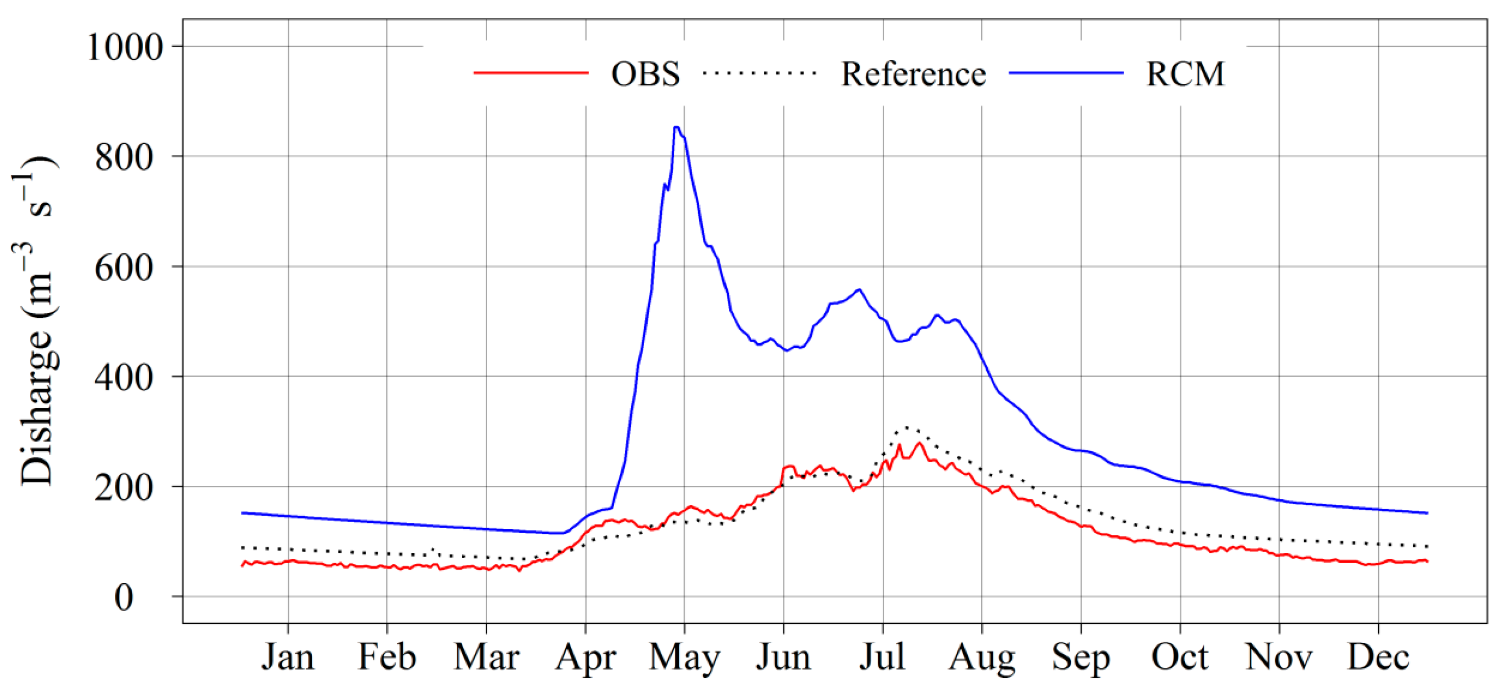
The mean daily cycle results reveal that the simulation run by original RCM precipitation and temperature has obvious bias and great overestimation for discharges (Figure 3), particularly in the wet seasons (April–September). This is to be expected because the performance of the RCM data is highly dependent upon the season. When the observed discharges are included, the original RCM-simulated discharges become less coherent. The NSE coefficient is −10.13 over the length of the relevant period, and this indicates that the original RCM outputs are not capable of being used for calibration and the bias cannot be corrected by hydrological calibration.

4.2. Validation of Original Precipitation and Temperature

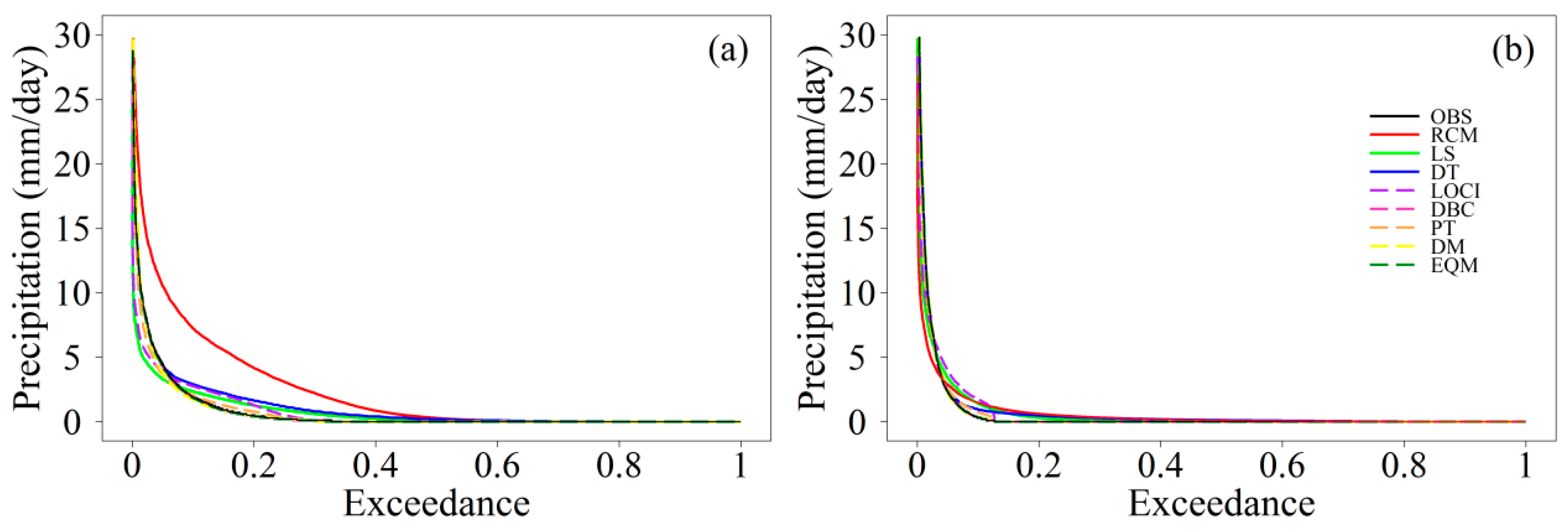
The validation of the original RCM-simulated precipitation and temperature is contingent on the quality of the probabilities distributions and average daily cycle. The subsequent discussion focuses upon the performance of daily average temperature because similar results are obtained from daily maximum and minimum temperatures. The performance of the RCM outputs is also dependent upon the specific region. The distribution of RCM-simulated precipitation at the BYBLK station is less coherent than observations obtained from the BLT station (Figure 4).
At the BYBLK station, overestimations are observed in RCM-simulated precipitation, with probabilities that fall below 0.78. When the focus is on the temporal distribution (
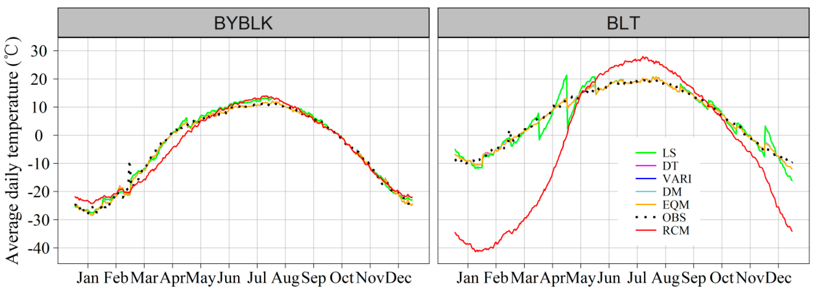
Figure 5), overestimated periods are mainly concentrated in the wet season. But the biases cannot be attributed to systematical error because the conditions are very different at the BLT station. RCM simulations underestimate precipitation, with probabilities below 0.04 and, when applied at the BLT station, overestimate probabilities between 0.04 and 0.80. The underestimations mainly occur during the June-July period and overestimations are concentrated in the November-December period. It is worthwhile to note that, in comparison to the dry season, precipitation is consistently less accurate in the wet season. This can possibly be attributed to the RCMs evidencing diminished capacity in the simulation of convective precipitation [
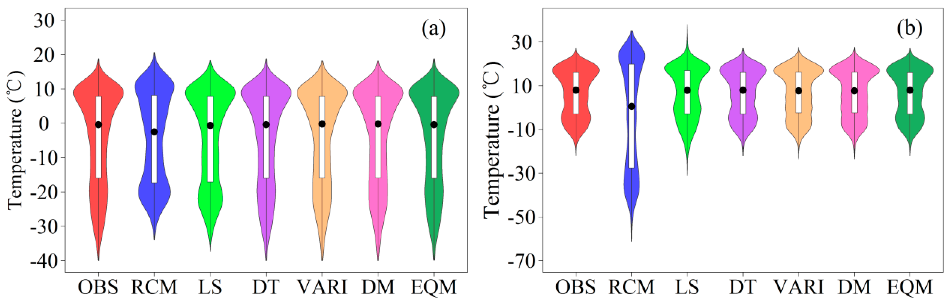
40]. The RCM-simulated temperature outputs obtained at the BYBLK station are more reliable than at the BLT station (Figure 6). The probabilities distribution of temperature at BYBLK is more concentrated and there are obvious overestimations of low temperatures that fall beneath −19.1 °C (probabilities above 0.8). High temperatures fall in the slightly overestimated range between 18.8 °C and 7.1 °C (probabilities below 0.28). Overestimations are mainly concentrated in the Winter and Summer seasons, while underestimations are clearly evidenced in Spring once temporal variation is taken into account (Figure 7). At the BLT station, the temperature is more decentralized and serious underestimations range between −21.9 °C and 13 °C (probabilities 0.37-1) during the November–May period. Slight overestimations fall between 13 °C to 27.1 °C (probabilities below 0.37) during the June–September period.

4.3. Validation of Corrected Precipitation and Temperature

All bias correction methods are capable of effectively improving the original RCM simulations to a certain degree. The LS and LOCI methods underestimate heavy precipitation, with probabilities falling below 0.08 and 0.06 at the BYBLK station, respectively. This is because the LS and LOCI are mean-based methods that adjust different precipitation levels by using a unique scaling factor during a specific month. Extreme precipitation is not specifically considered by the two methods. Meanwhile, overestimations are included, with probabilities falling between 0.08 and 0.33 in the LS method and 0.06 to 0.31 in the LOCI method. But the LOCI method is obviously superior when dry days (<0.1 mm) are considered. The LS method is limited in reproducing dry days and consistently overestimates probabilities that range from 0.33 to 0.79.
The DT method is able to competently adjust the higher precipitation in probabilities that fall below 0.06, but it does not take into account drizzle days corrections, and this results in consistent overestimations of probabilities between 0.31 and 0.79. It is fortunate that this limitation is fully overridden by the DBC method, which uses observations to correct the original RCM-simulated precipitation distribution to a completely uniform configuration. The DM, EQM, and PT methods reproduce precipitation quite well, with the partial exception of the PT method, which slightly overestimates the original precipitation within a probabilities range of 0.09–0.30. These corrected methods present similar capacities, both at the BLT and BYBLK station. But it is worth noticing that several outliers (extreme values) are evidenced within the DM and PT (the reason for this will be discussed at a later stage of this paper).
The performance of the corrected temperature confirms that all the temperature correction methods improve the original RCM simulations. The DM, DT, EQM, and VARI methods correct the original temperature and produce exceedance probabilities that closely resemble observations taken from the two stations. But the LS method, in particular when it is applied at the BLT station, is incapable of improving the RCM quality to the same extent as the other four methods. The poor performance of the original RCM-simulated temperature at the BLT station is still not fully overcome by the LS method, and this indicates the RCM-model dependence of the bias correction methods.
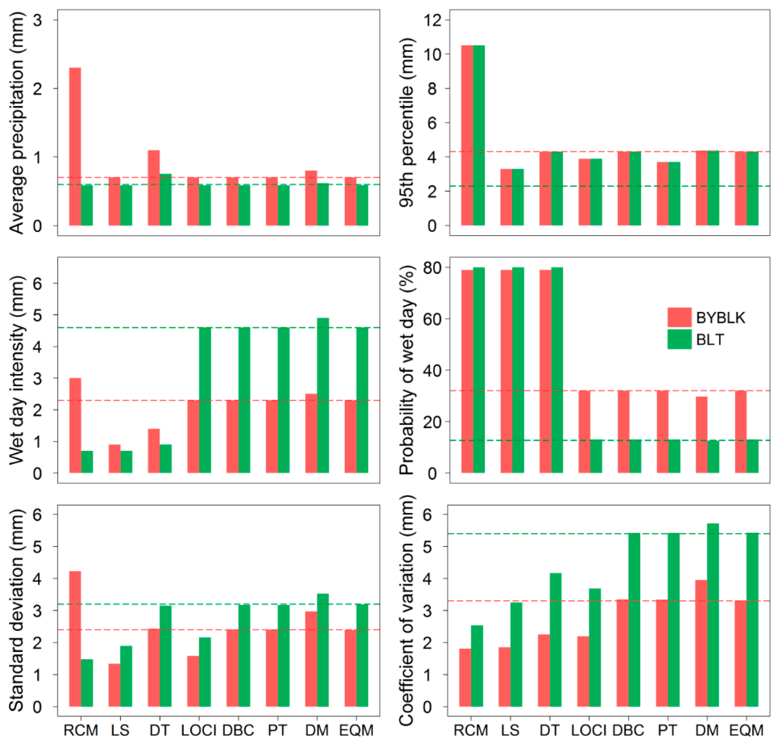
The calculated performance metrics (Figure 8) suggest that a bias in average precipitation is no longer evidenced in the LS method, whereas original RCM simulations respectively show a bias of 1.4 mm and −0.01 mm at the BYBLK and BLT stations. But the LS method still presents large biases in other indices. The DT method is capable of reproducing the 95th percentile upon the basis of the 100-quantile corrected processes, but it does not present great improvement in other metrics and its complete oversight of drizzle days means that it even extends the error in mean. Biases in mean precipitation, probability of wet days, and wet-day intensity are not found in the LOCI method, while biases in the coefficient of variation, 95th percentiles, and standard deviation still exist. The other four correction methods evidence a level of performance that exceeds each of these three methods. No bias in these metrics can be identified in the DBC and EQM methods, while their DM and PT counterparts only evidence slight biases in some metrics.
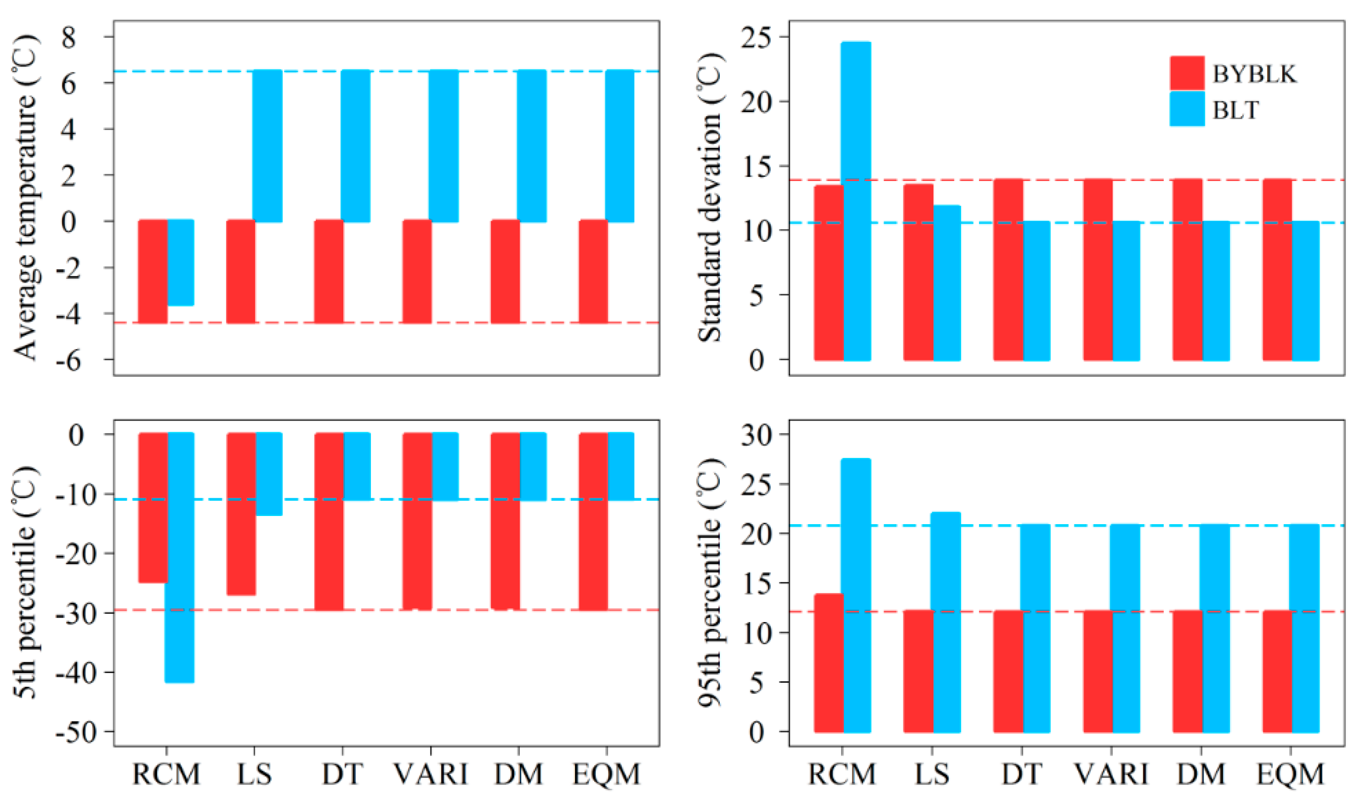
The bias in average temperature is no longer found in all correction methods at the two stations, whereas the original RCM temperature respectively presented biases of −0.03 °C and 10.14 °C at the BYBLK and BLT stations (Figure 9). The VARI method is the only one of the five temperature correction methods that specifically considers the correction of variance. In most cases, the correction in mean values does affect the variance, and this leads to variations in the DM, DT, and EQM methods, thereby lending coherence to the variance of observations and VARI-corrected temperature. The LS method also reduces the bias in variance, although it is unable to correct extreme temperatures (5/95th percentiles). The performance of the other four correction methods is broadly comparable and does not evidence biases in extreme temperatures.
The time-series-based metrics of these corrected precipitation and temperature data, along with original RCM simulations, are also analyzed in this paper (Figure 6 and Figure 7; Table 3). For presentational reasons, Table 3 only presents the results of the BYBLK station. The performance of RCM-simulated precipitation is very biased, as an MAE of 1.65 mm, NSE of −5.71, PBIAS of 224.2%, and R2 of 0.59 attests (daily scale). Comparison of these time-series-based metrics suggests that all methods are capable of improving the original RCM simulations to different levels. The DT method still overestimates precipitation, with PBIAS and MAE respectively rising to 49.50% and 0.47 mm. Other corrected precipitation series suggest that the MAE, PBIAS, NSE, and R2 respectively range between 0.27 mm/0.37 mm, −0.2%/4.2%, 0.46/0.72, and 0.56/0.72. In time-series-based metrics, the performance of mean-based methods (LS and LOCI) in precipitation is slightly better than quantile-based methods. Temperature exhibits a much better performance than precipitation at the BYBLK station, which slightly overestimates the observations with an MAE of 1.99 °C and PBIAS of 0.7%. All temperature bias correction methods improve the performance of RCM-simulated temperature and present PBIAS almost equal to zero.

4.4. The Performance of Bias Correction Methods for Hydrological Modelling

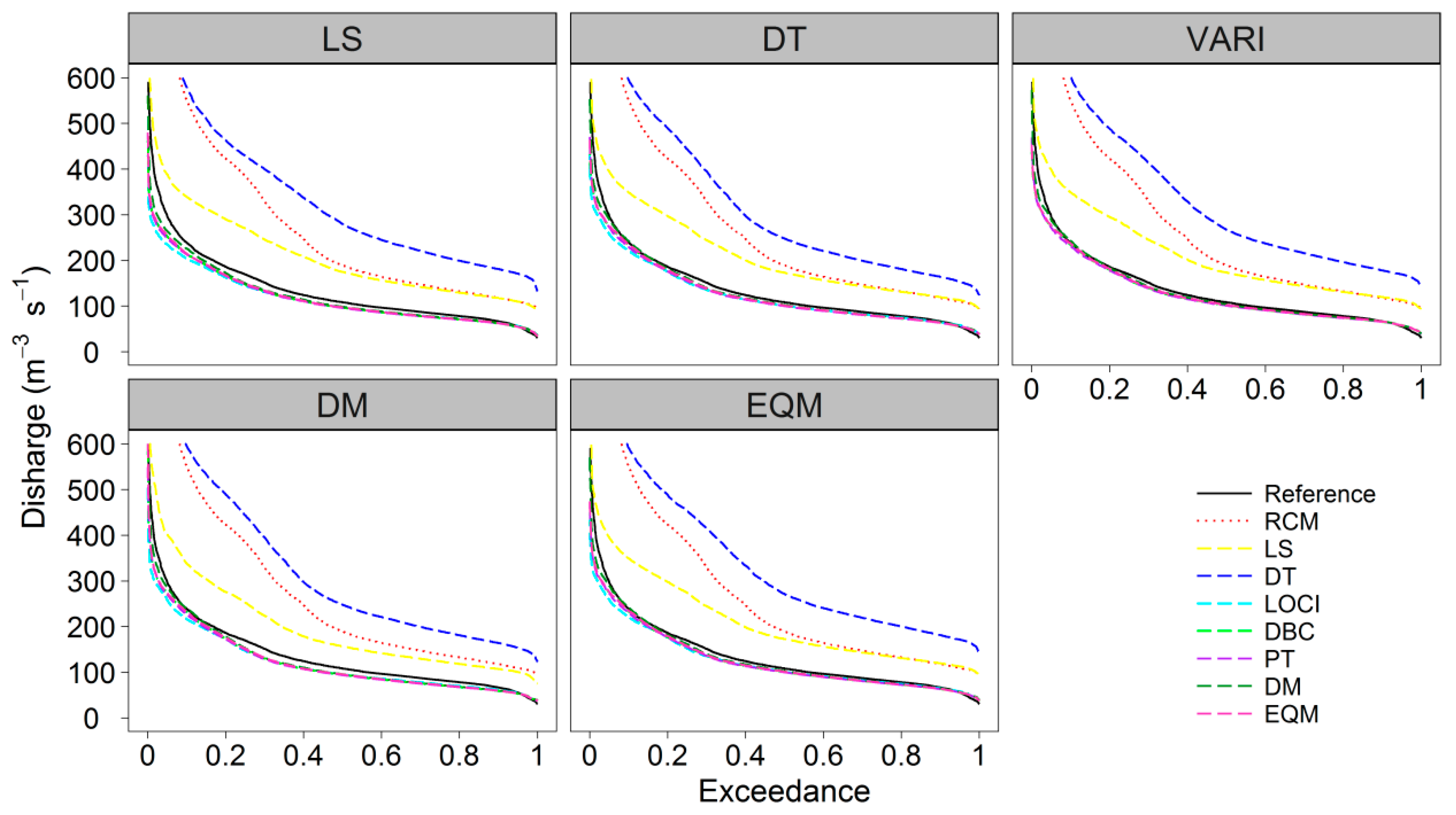
In order to evaluate the capacity of the corrected precipitation and temperature data in discharge simulations, 35 possible combinations of corrected precipitation and temperature data are applied to drive the SWAT model. The exceedance probabilities of simulated discharges are grouped in accordance with different temperature-corrected methods (Figure 10). The simulated discharges that use observed precipitation and temperature data, as opposed to observed discharges, are used as the reference in order to prevent the model exerting undue influence. Great uncertainty corresponds to different precipitation methods, and this is mainly attributable to the poor performance of DT and LS methods. Discharges simulated by the corrected precipitation with the LS and DT methods significantly differ with the reference. In particular, simulated discharges driven by corrected precipitation with the DT method are even worse than the discharges using original RCM-simulated precipitation.
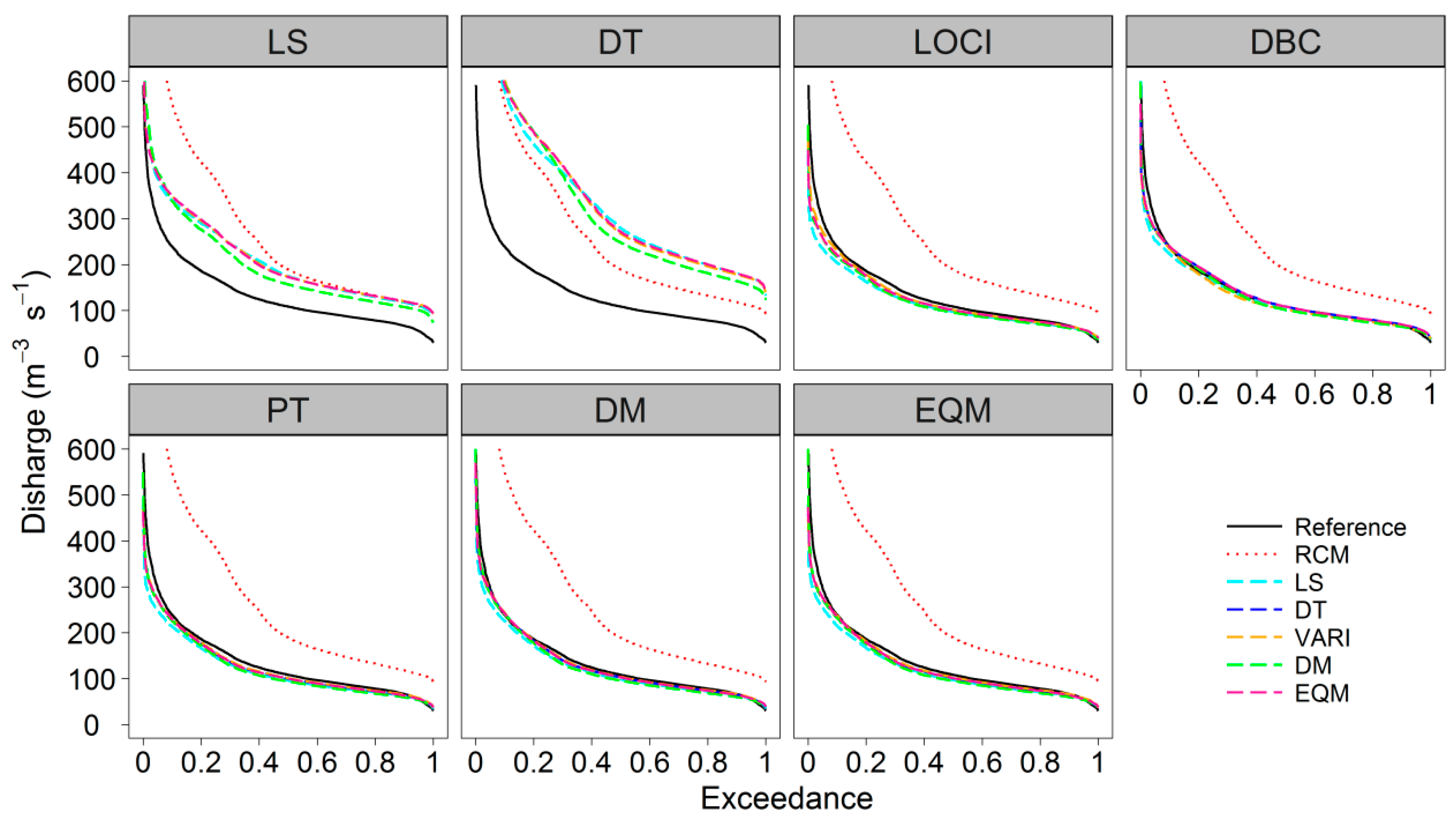
The DBC performs slightly better than the LOCI method when projecting the exceedance probabilities of discharges. The DM, EQM, and PT methods demonstrate a consistently good performance when reproducing the daily discharges, and there are no obvious differences between the three methods in this regard. Differences will be evaluated by applying statistical metrics in the following sections. In a similar manner to its immediate predecessor, Figure 11 presents the exceedance probability of simulated discharges, which are grouped in accordance with different precipitation correction methods. No substantial difference is found between the different temperature correction methods in hydrological modelling and a relatively small variability range is identified. This indicates that the temperature correction methods, in comparison to precipitation correction methods, provide a higher level of certainty in the reproduction of discharges. But the performances of these temperature-corrected methods are also slightly different when combined with different precipitation-corrected methods. When grouped with LOCI, DBC, PT, DM, and EQM-corrected methods for precipitation, these five temperature correction methods present quite similar forms, although the DM method evidences more differences than its other four counterparts when combined with the DT and LS methods—this may conceivably be attributed to the interaction included in the different method combinations.
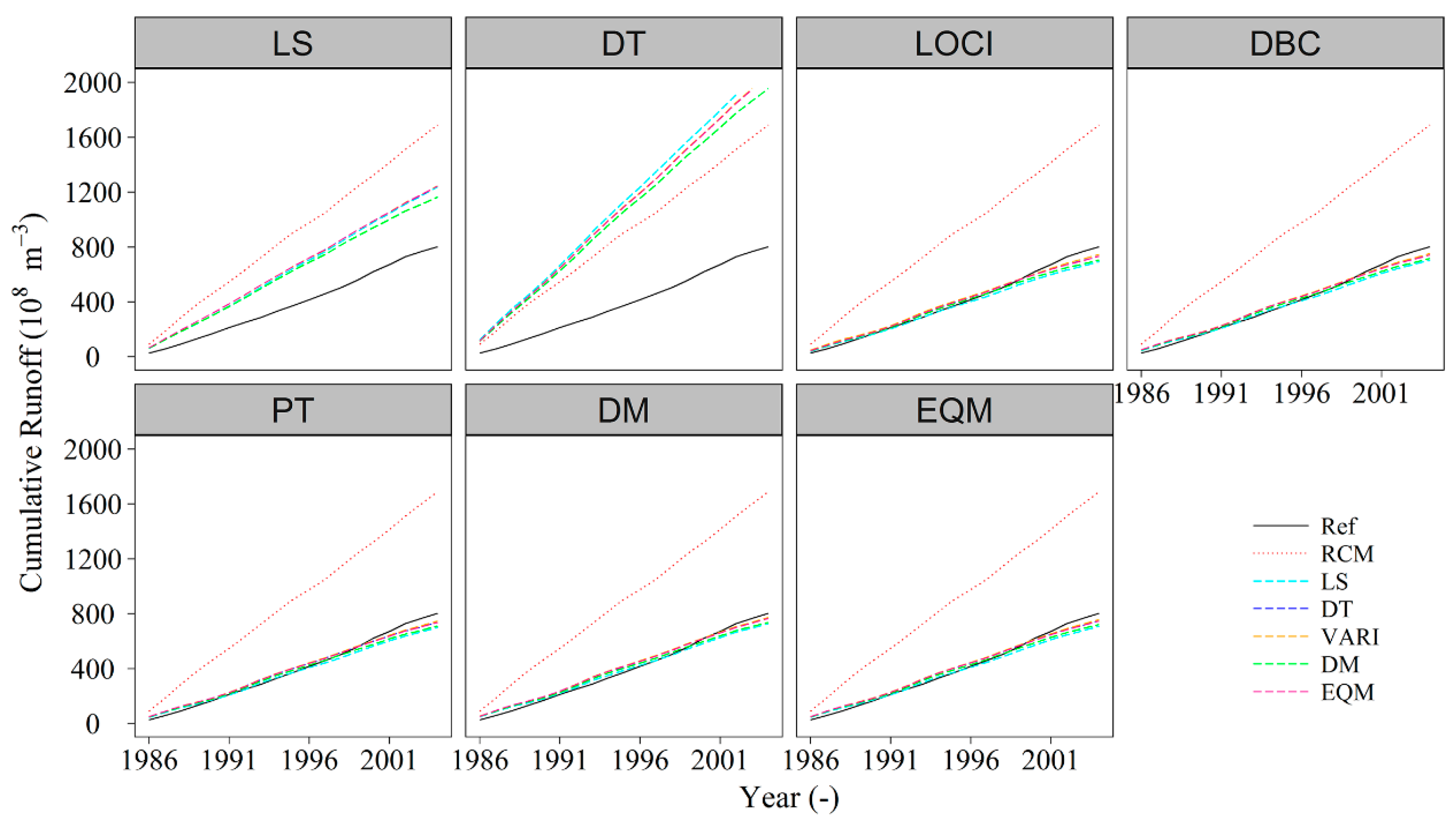
The cumulative runoff from 1986 to 2004 simulated by the 35 combinations is also presented in Figure 12 for better understanding the capacities of these bias correction methods in simulating interannual variabilities of discharge. The precipitation corrected by LS and DT methods is not able to catch the cumulative runoff well. The positive deviation is getting larger and larger from 1986 to 2004. The bias correction methods without wet-day frequency correction are unable to describe the interannual variabilities of discharge as well. The precipitation corrected by DM and EQM methods exhibited an obvious advantage when compared to precipitation corrected by LOCI, DBC, and PT methods, especially combined with temperature corrected by VARI and EQM. It indicates that these two methods are able to simulate the interannual variabilities of runoff effectively. The bias correction methods of precipitation also exhibited relative greater uncertainties in interannual variabilities of runoff when compared with temperature correction methods.
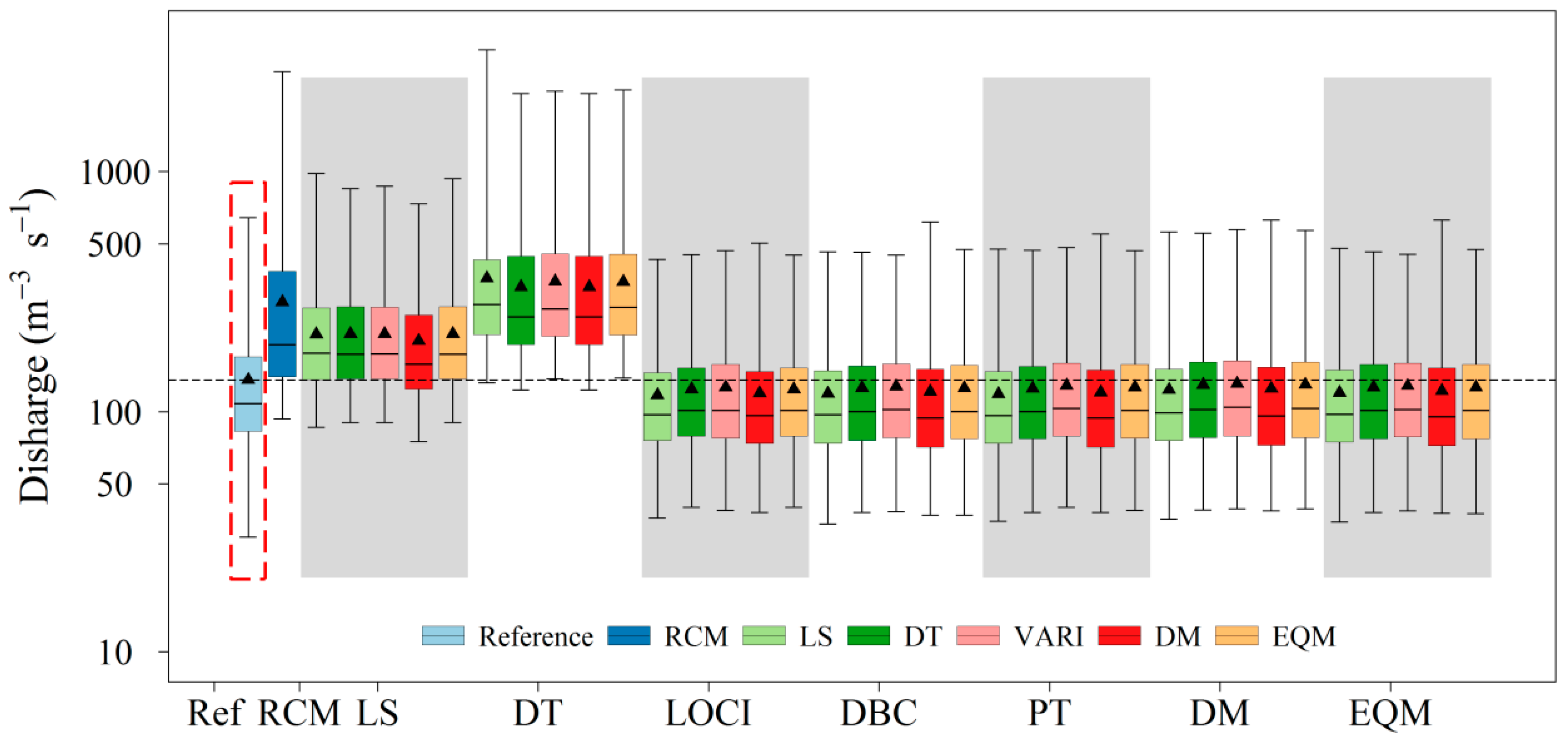
The SWAT-simulated discharge characteristics, including daily flood peaks, daily low flow, mean, and 25th quantile and 75th quantile discharges during the relevant period, are also considered (Figure 13). Simulations forced by corrected precipitation with the DT and LS methods generally seriously overestimate all these statistical indices, and this indicates that the precipitation correction methods without wet-day frequency correction are restricted to discharge simulations. Simulations conducted through corrected precipitation with the other five methods come very close to being referenced, especially when combined with temperature corrected by the DT, EQM, and VARI methods. In particular, the DM method for both precipitation and temperature corrections presents a slightly better performance in daily extreme flow simulations.
Table 4 summarizes the time-series-based metrics of simulated discharges forced by different combinations of corrected precipitation and temperature and original RCM outputs. With the exception of simulations driven by corrected precipitation with the DT method, all 35 simulations improved the statistical metrics. The simulations forced by corrected precipitation with the LS method are also very biased, with PBIAS ranging between 45.2% and 55.3%. The simulations that use corrected precipitation with the DBC, DM, EQM, LOCI, and PT methods more closely resemble simulations forced by observations with considerably reduced MAE and PBIAS. The corrected precipitation with the DM and EQM methods presents an equally excellent performance, while corrected temperature by the EQM and VARI methods performs best in the reproduction of time-series-based metrics. In the reproduction of discharges, the best combinations are the DM-corrected precipitation and VARI-corrected temperature.

5. Discussion

Several bias correction methods have been proposed to downscale RCM outputs as a prerequisite for the analysis of climate change. These methods range from simple linear scaling techniques to rather more sophisticated distribution mapping techniques. There is a clear and ongoing need to compare and evaluate their performance.
Numerous studies prove that the original RCM outputs, and in particular RCM-simulated precipitation [41,42,43], are always biased. Their direct use in climate change effects is inadvisable because they might lead to misleading results. The validating results of the original RCM simulations in this study indicate that the performance of RCM outputs varies across region. They fail in hydrological modelling because of their poor performance in the Kaidu River Basin and model calibration could not even overcome their biases. What is worth noting is that precipitation presents a consistently worse accuracy in the wet season than the dry season. The possible reason for this is that the RCMs have a diminished capacity in simulating convective precipitation [40].
All methods can improve the original RCM simulations at different levels. The LS method is the simplest bias correction method that corrects the climate data upon the basis of the difference between RCM simulations and observations. While it can adjust mean values, it cannot be used in the analysis of extreme events because the unique scaling factor in a specific month often leads to heavy precipitation being greatly underestimated [44]. The LOCI method is the extension of the LS method that effectively corrects the precipitation frequency. No bias can be found in wet-day frequency or intensity. When compared to the LS method, heavy precipitation is also partly corrected, and this is attributable to the correction in wet-day frequency. The DBC and DT methods are both based on 100-quantile distributions and their major point of divergence originates within the correction of precipitation occurrence [8]. The extreme events are perfectly presented within these two methods, and this feature clearly distinguishes them from the LOCI and LS methods.
However, the DT method greatly deviates the actual mean precipitation and produces large biases in discharge simulations. The EQM method is based on a point-wise empirical distribution and it takes different precipitation levels into account on an individual basis. In this study, the DBC and EQM methods perform the best in precipitation projection—this is because no bias is included in their frequency-based metrics. The nonlinear DM (based on Gamma distribution) and PT methods still evidence tiny biases in some frequency-based metrics. Meanwhile, the DM method should be used with caution because it originates within the assumption that RCM-simulated and observed time series approximate the distribution [45]. Its use is oppositional unless the time series obeys a theoretical distribution. As has already been noted, several extreme events are found in the corrected time series when the DM and PT methods are used and these new extremes arise when the reference period is not stable [4]. Therefore, a long and relatively stable period would be preferable as it would avoid extreme error to the greatest possible extent.
When time-series-based metrics are included, linear-based LS and LOCI methods perform best, with the nonlinear-based PT method following closely behind. Distribution-based methods evidence a poorer level of performance than other methods. A study by Fang, Yang, Chen and Zammit [29] reached a similar conclusion—these bias correction methods are grounded within temporal structure correction [13,30], while linear approaches perform slightly better than the other approaches. In the case of precipitation correction, the LS method demonstrates the poorest performance in frequency-based and time-series-based metrics and is clearly distinguished from the other four methods when applied to temperature correcting. This is because the time structure problem does not exist in temperature series. The nonlinear VARI method and distribution-based DM, DT, and EQM methods compare fairly well, and present a similar performance of PBIAS equal to zero.
When the corrected precipitation and temperature are transferred to discharges by hydrological modelling, great improvements are evidenced that compare favorably to the results forced by original RCM outputs (corrected precipitation with the DT method being the one exception in this respect). Different precipitation-corrected methods present larger uncertainty when compared against various temperature-corrected methods—this is attributable to the poor performance of these methods in the absence of wet-day frequency correction. The exceedance probabilities of simulated discharges driven by corrected precipitation with the DT method greatly deviate the references, to an extent that even exceeds the simulated discharges driven by the original RCM outputs. The results can be traced back to two sources. In the first instance, simulated discharges driven by the original RCM outputs were calibrated specifically and the biases were partly overcome as a consequence.
Chen, Brissette, Chaumont and Braun [13] arrive at a similar conclusion. The model may also be sensitive to a bias in the DT method’s corrected precipitation that has been further magnified by hydrological modelling. The corrected precipitation in the LS method for precipitation was also not acceptable for the hydrological modelling because it includes large biases. This further reiterates that the drizzle effects were not neglected and that the methods without wet-day frequency correction, such as those evidenced in the DT and LS methods, are not acceptable in discharge simulations in our study area.
These results clearly diverge from a previous study by Chen, Brissette, Chaumont and Braun [4], which found that the drizzle effects are not significant in North America. It indicates that the DT method is highly dependent on the RCM and region. It performs better in the more humid North America than in arid Xinjiang, which has less precipitation occurrences. The other five methods are all capable of reproducing discharges to a reasonable extent. Discharges simulated by corrected precipitation with the DBC method perform slightly better when compared against discharges simulated by corrected precipitation with the LOCI method. Although correction based on 100 quantiles does affect hydrological modelling, the effects are not comparable to those evidenced for wet-day frequency correction. DM and EQM methods perform better against other methods when applied to corrected precipitation; the same applies to EQM and VARI methods in relation to corrected temperature. The performance of these correction methods in relation to discharge simulations is not completely consistent with those for climate projection; nonetheless, this is only a small difference, which attests to the robust performance of these methods.
The Kaidu River Basin is a snow-dominated basin where melting water accounts for 58.6% of the total discharges. Discharges are therefore less sensitive to the temporal structure of precipitation occurrences. Chen, Brissette, Chaumont and Braun [13] also suggest that bias correction methods perform more poorly in precipitation-dominated regions than in the snow-dominated regions. The weak performance of the time structure of corrected precipitation may therefore be insufficiently recognized by this study. Lafon, Dadson, Buys and Prudhomme [42] also suggest that corrected precipitation is more sensitive to the selection of a particular time period. Bias correction methods should therefore be used with caution when the studies are strongly dependent on the temporal structure of precipitation, although it should be recognized that a good temporal structure of the original RCM simulations provides considerable assurance in this respect.

6. Conclusions

This paper compares the performances of (seven precipitation and five temperature bias) RCM correction methods and their hydrological applications in China’s Kaidu River Basin. The abilities of these corrected methods are evaluated by reproducing discharges, precipitation, and temperature through the SWAT hydrological model. Several conclusions can be extracted afterwards.
Original RCM outputs are very biased, and this precludes their direct use in the analysis of climate change effects. The representation of the RCM simulations is highly dependent upon the region and season. All bias correction methods have the potential to improve the performance of reproducing precipitation and temperature, although the bias correction method great influences their final results.
The performance of different precipitation-corrected methods presented greater differences when compared against various temperature-corrected methods. These differences mainly resulted from the poor performance of the corrected methods (DT and LS methods) in the absence of precipitation occurrence correction. The distribution-based DBC and EQM methods performed best in reproducing precipitation, while all temperature-corrected methods, with the exception of the LS method, performed extremely well.
The correction in wet-day frequency is extremely important for hydrological projection of the Kaidu River Basin. The DT and LS methods, which lack wet-day frequency correction, are not suitable for being applied in discharge simulations. Biases in corrected precipitation are likely amplified when transferred to discharges. The distribution-based DM and EQM methods for precipitation performed equally well in discharge simulations. There were no substantial differences in the various temperature-corrected methods in discharge simulations, while the LS method clearly provided the poorest performance when compared against the other methods. The EQM and VARI methods for temperature did the best job in discharge simulation. The DM method for both precipitation and temperature evidenced a narrow superiority in extreme-flow projection.
In general, this paper emphasizes the importance of using several bias correction methods for crosscheck in climate and hydrological response analysis. Even the performance of bias correction methods is dependent upon the RCM model and region. The results set out in this paper are of wider significance and the procedures can accordingly be applied to other regions.

Author Contributions

Tie Liu, Anming Bao, Amaury Frankl and Fanhao Meng conceived and designed the experiments of this study; Min Luo, Fanhao Meng and Yongchao Duan collected and processed the data; Min Luo, Yongchao Duan and Fanhao Meng calibrated and validated the model; Min Luo analysed the results and wrote the paper. All authors have proofread and approved the final manuscript.

Acknowledgments

This work was founded by State’s Key Project of Research and Development Plan (Grant No. 2017YFC0404501), National Natural Science Foundation of China (Grant No.U1503183), International Partnership Program of the Chinese Academy of Sciences (Grant No. 131551KYSB20160002), the Tianshan Innovation Team Project of Xinjiang Department of Science and Technology (Grant No. Y744261), Strategic Priority Research Program of Chinese Academy of Sciences, Pan-Third Pole Environment Study for a Green Silk Road (Grant No. XDA2006030302) and the APC was funded by the the Tianshan Innovation Team Project of Xinjiang Department of Science and Technology (Grant No. Y744261). M.L. was supported by grants from the China Scholarship Council (201604910973).

Conflicts of Interest

The authors declare that there are no conflicts of interest regarding the publication of this paper.

References

  1. Mpelasoka, F.S.; Chiew, F.H. Influence of rainfall scenario construction methods on runoff projections. J. Hydrometeorol. 2009, 10, 1168–1183. [Google Scholar] [CrossRef]
  2. Teutschbein, C.; Seibert, J. Regional climate models for hydrological impact studies at the catchment scale: A review of recent modeling strategies. Geogr. Compass 2010, 4, 834–860. [Google Scholar] [CrossRef] [Green Version]
  3. Buonomo, E.; Jones, R.; Huntingford, C.; Hannaford, J. On the robustness of changes in extreme precipitation over Europe from two high resolution climate change simulations. Q. J. R. Meteorol. Soc. 2007, 133, 65–81. [Google Scholar] [CrossRef] [Green Version]
  4. Chen, J.; Brissette, F.P.; Chaumont, D.; Braun, M. Performance and uncertainty evaluation of empirical downscaling methods in quantifying the climate change impacts on hydrology over two North American river basins. J. Hydrol. 2013, 479, 200–214. [Google Scholar] [CrossRef]
  5. Turco, M.; Llasat, M.C.; Herrera, S.; Gutiérrez, J.M. Bias correction and downscaling of future rcm precipitation projections using a mos-analog technique. J. Geophys. Res. Atmos. 2017, 122, 2631–2648. [Google Scholar] [CrossRef]
  6. Durman, C.; Gregory, J.M.; Hassell, D.C.; Jones, R.; Murphy, J. A comparison of extreme European daily precipitation simulated by a global and a regional climate model for present and future climates. Q. J. R. Meteorol. Soc. 2001, 127, 1005–1015. [Google Scholar] [CrossRef]
  7. Herrera, S.; Fita, L.; Fernández, J.; Gutiérrez, J. Evaluation of the mean and extreme precipitation regimes from the ensembles regional climate multimodel simulations over Spain. J. Geophys. Res. Atmos. 2010, 115, D21117. [Google Scholar] [CrossRef]
  8. Teutschbein, C.; Seibert, J. Bias correction of regional climate model simulations for hydrological climate-change impact studies: Review and evaluation of different methods. J. Hydrol. 2012, 456, 12–29. [Google Scholar] [CrossRef]
  9. Zollo, A.L.; Rianna, G.; Mercogliano, P.; Tommasi, P.; Comegna, L. Validation of a simulation chain to assess climate change impact on precipitation induced landslides. In Landslide Science for a Safer Geoenvironment; Springer: Cham, Switzerland, 2014; pp. 287–292. [Google Scholar]
  10. Crochemore, L.; Ramos, M.-H.; Pappenberger, F. Bias correcting precipitation forecasts to improve the skill of seasonal streamflow forecasts. Hydrol. Earth Syst. Sci. 2016, 20, 3601–3618. [Google Scholar] [CrossRef] [Green Version]
  11. Lenderink, G.; Buishand, A.; Deursen, W.V. Estimates of future discharges of the river rhine using two scenario methodologies: Direct versus delta approach. Hydrol. Earth Syst. Sci. 2007, 11, 1145–1159. [Google Scholar] [CrossRef]
  12. White, R.; Toumi, R. The limitations of bias correcting regional climate model inputs. Geophys. Res. Lett. 2013, 40, 2907–2912. [Google Scholar] [CrossRef] [Green Version]
  13. Chen, J.; Brissette, F.P.; Chaumont, D.; Braun, M. Finding appropriate bias correction methods in downscaling precipitation for hydrologic impact studies over North America. Water Resour. Res. 2013, 49, 4187–4205. [Google Scholar] [CrossRef] [Green Version]
  14. Luo, M.; Liu, T.; Frankl, A.; Duan, Y.; Meng, F.; Bao, A.; Kurban, A.; De Maeyer, P. Defining spatiotemporal characteristics of climate change trends from downscaled gcms ensembles: How climate change reacts in Xinjiang, China. Int. J. Climatol. 2018, 38, 2538–2553. [Google Scholar] [CrossRef]
  15. Liu, T.; Willems, P.; Pan, X.; Bao, A.M.; Chen, X.; Veroustraete, F.; Dong, Q. Climate change impact on water resource extremes in a headwater region of the Tarim Basin in China. Hydrol. Earth Syst. Sci. 2011, 15, 6593–6637. [Google Scholar] [CrossRef]
  16. Chen, Z.; Chen, Y.; Li, B. Quantifying the effects of climate variability and human activities on runoff for Kaidu River Basin in arid region of northwest China. Theor. Appl. Climatol. 2013, 111, 537–545. [Google Scholar] [CrossRef]
  17. Dou, Y.; Chen, X.; Bao, A.; Li, L. The simulation of snowmelt runoff in the ungauged kaidu river basin of Tianshan Mountains, China. Environ. Earth Sci. 2011, 62, 1039–1045. [Google Scholar] [CrossRef]
  18. Fang, G.; Yang, J.; Chen, Y.; Li, Z.; De Maeyer, P. Impact of gcm structure uncertainty on hydrological processes in an arid area of China. Hydrol. Res. 2017, 48, nh2017227. [Google Scholar] [CrossRef]
  19. Xu, J.; Chen, Y.; Li, W.; Peng, P.Y.; Yang, Y.; Wei, C.; Hong, Y. Combining bpann and wavelet analysis to simulate hydro-climatic processes—A case study of the Kaidu River, northwest China. Front. Earth Sci. 2013, 7, 227–237. [Google Scholar] [CrossRef]
  20. Xu, J.; Chen, Y.; Ji, M.; Lu, F. Climate change and its effects on runoff of Kaidu River, Xinjiang, China: A multiple time-scale analysis. Chin. Geogr. Sci. 2008, 18, 331–339. [Google Scholar] [CrossRef]
  21. Chen, Z.; Chen, Y. Effects of climate fluctuations on runoff in the headwater region of the Kaidu River in northwestern China. Front. Earth Sci. 2014, 8, 309. [Google Scholar] [CrossRef]
  22. Baek, H.-J.; Lee, J.; Lee, H.-S.; Hyun, Y.-K.; Cho, C.; Kwon, W.-T.; Marzin, C.; Gan, S.-Y.; Kim, M.-J.; Choi, D.-H. Climate change in the 21st century simulated by hadgem2-ao under representative concentration pathways. Asia-Pac. J. Atmos. Sci. 2013, 49, 603–618. [Google Scholar] [CrossRef]
  23. Mearns, L.O.; Gutowski, W.; Jones, R.; Leung, R.; McGinnis, S.; Nunes, A.; Qian, Y. A regional climate change assessment program for North America. Eos Trans. Am. Geophys. Union 2009, 90, 311. [Google Scholar] [CrossRef]
  24. Schmidli, J.; Frei, C.; Vidale, P.L. Downscaling from gcm precipitation: A benchmark for dynamical and statistical downscaling methods. Int. J. Climatol. 2006, 26, 679–689. [Google Scholar] [CrossRef]
  25. Fowler, H.; Ekström, M.; Blenkinsop, S.; Smith, A. Estimating change in extreme European precipitation using a multimodel ensemble. J. Geophys. Res. Atmos. 2007, 112, D18104. [Google Scholar] [CrossRef]
  26. Bi, E.G.; Gachon, P.; Vrac, M.; Monette, F. Which downscaled rainfall data for climate change impact studies in urban areas? Review of current approaches and trends. Theor. Appl. Climatol. 2017, 127, 685–699. [Google Scholar]
  27. Leander, R.; Buishand, T.A.; van den Hurk, B.J.; de Wit, M.J. Estimated changes in flood quantiles of the river meuse from resampling of regional climate model output. J. Hydrol. 2008, 351, 331–343. [Google Scholar] [CrossRef]
  28. Terink, W.; Hurkmans, R.; Torfs, P.; Uijlenhoet, R. Evaluation of a bias correction method applied to downscaled precipitation and temperature reanalysis data for the rhine basin. Hydrol. Earth Syst. Sci. 2010, 14, 687–703. [Google Scholar] [CrossRef] [Green Version]
  29. Fang, G.; Yang, J.; Chen, Y.; Zammit, C. Comparing bias correction methods in downscaling meteorological variables for a hydrologic impact study in an arid area in China. Hydrol. Earth Syst. Sci. 2015, 19, 2547–2559. [Google Scholar] [CrossRef] [Green Version]
  30. Chen, J.; Brissette, F.P.; Poulin, A.; Leconte, R. Overall uncertainty study of the hydrological impacts of climate change for a Canadian watershed. Water Resour. Res. 2011, 47, W12509. [Google Scholar] [CrossRef]
  31. Piani, C.; Haerter, J.; Coppola, E. Statistical bias correction for daily precipitation in regional climate models over Europe. Theor. Appl. Climatol. 2010, 99, 187–192. [Google Scholar] [CrossRef]
  32. Thom, H.C. A note on the gamma distribution. Mon. Weather Rev. 1958, 86, 117–122. [Google Scholar] [CrossRef]
  33. Piani, C.; Weedon, G.; Best, M.; Gomes, S.; Viterbo, P.; Hagemann, S.; Haerter, J. Statistical bias correction of global simulated daily precipitation and temperature for the application of hydrological models. J. Hydrol. 2010, 395, 199–215. [Google Scholar] [CrossRef]
  34. Ines, A.V.; Hansen, J.W. Bias correction of daily gcm rainfall for crop simulation studies. Agric. For. Meteorol. 2006, 138, 44–53. [Google Scholar] [CrossRef]
  35. Schoenau, G.J.; Kehrig, R.A. Method for calculating degree-days to any base temperature. Energy Build. 1990, 14, 299–302. [Google Scholar] [CrossRef]
  36. Jakob Themeßl, M.; Gobiet, A.; Leuprecht, A. Empirical-statistical downscaling and error correction of daily precipitation from regional climate models. Int. J. Climatol. 2011, 31, 1530–1544. [Google Scholar] [CrossRef]
  37. Arnold, J.G.; Srinivasan, R.; Muttiah, R.S.; Williams, J.R. Large area hydrologic modeling and assessment part I: Model development. J. Water Resour. Water Eng. 1998, 34, 73–89. [Google Scholar] [CrossRef]
  38. Luo, M.; Meng, F.; Liu, T.; Duan, Y.; Frankl, A.; Kurban, A.; De Maeyer, P. Multi–model ensemble approaches to assessment of effects of local climate change on water resources of the Hotan River Basin in Xinjiang, China. Water 2017, 9, 584. [Google Scholar] [CrossRef]
  39. Cibin, R.; Sudheer, K.; Chaubey, I. Sensitivity and identifiability of stream flow generation parameters of the swat model. Hydrol. Process. 2010, 24, 1133–1148. [Google Scholar] [CrossRef]
  40. Gudmundsson, L.; Bremnes, J.; Haugen, J.; Engen-Skaugen, T. Downscaling rcm precipitation to the station scale using statistical transformations—A comparison of methods. Hydrol. Earth Syst. Sci. 2012, 16, 3383–3390. [Google Scholar] [CrossRef]
  41. Maraun, D.; Wetterhall, F.; Ireson, A.; Chandler, R.; Kendon, E.; Widmann, M.; Brienen, S.; Rust, H.; Sauter, T.; Themeßl, M. Precipitation downscaling under climate change: Recent developments to bridge the gap between dynamical models and the end user. Rev. Geophys. 2010, 48, 633–650. [Google Scholar] [CrossRef]
  42. Lafon, T.; Dadson, S.; Buys, G.; Prudhomme, C. Bias correction of daily precipitation simulated by a regional climate model: A comparison of methods. Int. J. Climatol. 2013, 33, 1367–1381. [Google Scholar] [CrossRef] [Green Version]
  43. Kjellström, E.; Nikulin, G.; Hansson, U.; Strandberg, G.; Ullerstig, A. 21st century changes in the European climate: Uncertainties derived from an ensemble of regional climate model simulations. Tellus A 2011, 63, 24–40. [Google Scholar] [CrossRef]
  44. Haerter, J.; Hagemann, S.; Moseley, C.; Piani, C. Climate model bias correction and the role of timescales. Hydrol. Earth Syst. Sci. 2011, 15, 1065–1079. [Google Scholar] [CrossRef] [Green Version]
  45. Sun, F.; Roderick, M.L.; Lim, W.H.; Farquhar, G.D. Hydroclimatic projections for the murray-darling basin based on an ensemble derived from intergovernmental panel on climate change ar4 climate models. Water Resour. Res. 2011, 47, W00G02. [Google Scholar] [CrossRef]
Figure 1. Locations of the Kaidu River Basin, Bayinbuluke (BYBLK) and Baluntai (BLT) meteorological stations, as well as the Dashankou (DSK) hydrological station; inset maps show the locations of Xinjiang Autonomous Region within China and the Kaidu River Basin within Xinjiang.
Water 10 01046 g001
Figure 2. Mean daily precipitation, temperature, and pan evaporation at the BYBLK station and discharge at the DSK station.
Water 10 01046 g002
Figure 3. Average daily hydrographs for the observed discharges (OBS), simulated discharges using observed meteorological data (Reference), and simulated discharges using RCM data (RCM) at DSK stations during the reference period 1986–2004.
Water 10 01046 g003
Figure 4. Exceedance probabilities of the observed, RCM, and bias-corrected precipitation in BYBLK (a) and BLT (b) meteorological stations.
Water 10 01046 g004
Figure 5. The average daily precipitation cycle in the reference period (1965–2004) at BYBLK and BLT meteorological stations.
Water 10 01046 g005
Figure 6. Violin plots showing the frequency distributions of the probability density function for the observed, RCM, and bias-corrected temperature in BYBLK (a) and BLT (b) meteorological stations. White bars represent 25th–75th quantile values, and black dots indicate the median.
Water 10 01046 g006
Figure 7. The average daily temperature cycle in the reference period (1965–2004) at BYBLK and BLT meteorological stations.
Water 10 01046 g007
Figure 8. The wet day intensity, probability of wet days, 95th percentile, average precipitation intensity, standard deviation, and coefficient of variation at BYBLK and BLT meteorological stations in the period 1965–2004.
Water 10 01046 g008
Figure 9. The average temperature, 5th percentile temperature, 95th percentile temperature, and standard deviation at BYBLK and BLT meteorological stations in the period 1965–2004.
Water 10 01046 g009
Figure 10. Exceedance probabilities of discharge between 1986–2004 periods grouped by temperature bias-corrected methods.
Water 10 01046 g010
Figure 11. Exceedance probabilities of discharge between 1986–2004 periods grouped by precipitation bias-corrected methods.
Water 10 01046 g011
Figure 12. Cumulative runoff from 1986 to 2004 grouped by precipitation bias-corrected methods.
Water 10 01046 g012
Figure 13. Box plot of daily discharge intensity quantiles at the DSK station for those simulated using observed data, RCM data, and bias-corrected data grouped by precipitation corrected methods.
Water 10 01046 g013
Table 1. Bias correction methods for precipitation and temperature.
Bias Correction for PrecipitationBias Correction for Temperature
Linear scaling (LS)Linear scaling (LS)
Daily translation (DT)Daily translation (DT)
Local intensity scaling (LOCI)Variance scaling (VARI)
Daily bias correction (DBC)Distribution mapping (DM)
Power transformation (PT)Empirical Quantile Mapping (EQM)
Distribution mapping (DM)
Empirical Quantile Mapping (EQM)
Table 2. Sensitivity rate and final calibration values of the top ten selected SWAT model parameters.
ComponentParameter NameDescriptionSensitivity RateFinal Estimate Value
SnowSFTMPSnowfall temperature21.5
SMTMPSnow melt base temperature10.7
SMFMXMelt factor for snow on 21 June67.5
SMFMNMelt factor for snow on 21 December82.1
Subbasin conditionPLAPSPrecipitation lapse rate3183
TLAPSTemperature lapse rate4−7.8
Land use/coverOV_NManning’s “n” value for overland flow100.2
CNMoisture constitution II curve number568
River courseCH_N2Manning’s “n” value for the main channel90.18
CH_K2Effective hydraulic conductivity in main channel alluvium7240
Table 3. Time-series-based metrics of original and corrected precipitation as well as temperature on an average daily scale at the BYBLK station.
ParameterMethodMAE (mm/°C)PBIAS (%)NSE (−)R2 (−)
PrRCM1.65224.20−5.710.59
LS0.270.000.720.72
DT0.4749.500.290.65
LOCI0.29−0.200.690.69
DBC0.34−0.200.560.60
PT0.33−0.200.570.61
DM0.374.200.460.56
EQM0.340.000.560.60
TasRCM1.990.70.960.96
LS0.89−0.20.990.99
DT0.7600.990.99
VARI0.7800.990.99
DM0.7800.990.99
EQM0.7600.990.99
Table 4. Time-series-based metrics of simulated discharges forced by 35 combinations of corrected precipitation and temperature as well as original RCM simulations on an average daily scale at the DSK station.
Method (Pr)Method (Tas)MAE (m3s−1)PBIAS (%)NSE (−)R2 (−)Method (Pr)Method (Tas)MAE (m3s−1)PBIAS (%)NSE (−)R2 (−)
LSLS35.2654.60−0.880.70PTLS9.76−12.800.810.91
DT35.5655.20−0.730.86DT6.63−8.000.900.93
VARI35.7155.30−0.730.87VARI5.92−6.900.910.93
DM29.3745.20−0.330.87DM8.75−11.500.850.92
EQM35.5655.20−0.740.86EQM6.58−8.100.900.93
DTLS106.34165.00−17.350.21DMLS7.92−9.100.860.91
DT92.54143.60−12.090.63DT5.58−4.600.920.93
VARI101.05156.80−14.190.47VARI5.04−3.500.930.93
DM92.54143.60−12.090.63DM7.85−8.100.880.91
EQM100.62156.10−13.910.50EQM5.53−4.500.920.93
LOCILS10.10−13.800.790.91EQMLS9.15−11.700.830.91
DT6.62−8.700.890.94DT6.14−6.800.910.93
VARI5.92−6.900.910.93VARI5.49−5.600.920.93
DM8.37−1200.860.93DM8.22−10.100.870.92
EQM6.59−8.700.890.94EQM6.12−6.800.910.93
DBCLS9.45−12.200.820.91RCMRCM71.31110.60−10.130.42
DT6.37−7.400.900.93
VARI5.75−6.200.910.93
DM8.52−10.800.860.92
EQM6.33−7.400.910.93

