Quantitative Evaluation Method for Landscape Color of Water with Suspended Sediment

State Key Laboratory of Hydraulics and Mountain River Engineering, Sichuan University, Chengdu 610065, China
*
Author to whom correspondence should be addressed.
Water 2018, 10(8), 1042; https://doi.org/10.3390/w10081042
Submission received: 31 May 2018
/
Revised: 22 July 2018
/
Accepted: 30 July 2018
/
Published: 6 August 2018
(This article belongs to the Special Issue Water Quality: A Component of the Water-Energy-Food Nexus)
Abstract
:Landscape water is an important part of natural landscape, and a reasonable assessment of water landscape color is the basis for scientifically evaluating the quality of water landscape. To evaluate water landscape color with different concentrations of sediment objectively and quantitatively, a method of evaluating water landscape color based on hyperspectral technology is proposed to calculate water landscape color. The color spectrum calculation model of the water landscape color was constructed using the Commission Internationale de L’Eclairage spectrum three stimulus system (CIE-XYZ) calculation method and the response relationship among water reflectance, water depth, and sediment concentration. Under the conditions of eliminating as many external factors as possible, using a hyperspectral instrument to measure the reflectance of sediment and water, the response relationship between water depth and sediment concentration and water reflectance is calculated. Water depth and sediment concentration, which did not appear previously, were verified by experiments that proved the reliability of the water landscape color spectrum calculation model. By using different absolute value of chromatic coordinates in the international CIE-XYZ calculation method, a formula for determining the difference in sediment concentration for water landscape color was defined, and the quantitative evaluation method of landscape color of sand-laden water was established. In this research, we found that the predicted water landscape color, quantified by the color spectrum calculation model, is basically consistent with the actual color of landscape water and is basically in line with actual observation about significant difference assessment, which demonstrated the accuracy and reliability of the model. Hence, this research provides a scientific basis for the establishment of other water quality factors to evaluate water color, which makes it possible to quantify the color of the water landscape based on the establishment the color spectrum calculation model.
1. Introduction
Landscape water, an important part of the natural landscape, plays a very important role in water ecosystem, such as regulating regional temperature, reducing flood disasters, providing material basis for ecosystem diversity, and producing social and economic benefits [1,2]. At present, with the development of high-speed urbanization and industrialization, the landscape water is greatly threatened and the water quality has dropped significantly [3]. Landscape pollution of the water body is cloudy, with abnormal color, and seriously weakens the landscape function [4]. Besides, landscape pollution critically destroys the water ecosystem and has a great influence on the living environment of the nearby residents [5]. The rational evaluation of the water landscape color is the basis for the scientific evaluation of water landscape color. Therefore, the quantitative evaluation of water landscape color has important scientific significance and reference value for the quality assessment of landscape water and the formulation of effective measures to mitigate the impact of pollution on water landscapes.
Some research [6] shows that the pollution of water landscape color is mainly affected by organic matter, suspended particulates, nutrients and algae. Sediment is the most common non-dissolved matter, which can easily cause color variation in water landscape color. After the sediment particles enter the water body, they will migrate and diffuse because of the comprehensive effect of gravity, buoyancy, resistance and transverse turbulence. When the velocity of the sediment intervenes, an obvious sedimentation zone in landscape water will occur because of the slow velocity of the sediment transportation and diffusion [7,8]. To quantitatively analyze the influence of sedimentation zone on water landscape color, an effective method is needed to detect the influence of sediment on water landscape color. The detection methods of water chromaticity have been comparatively developed both at home and abroad. Referring to the international standard ISO 7887-1985 “Water quality-determination of color” [9], China has formulated the national standard detection method of water color (GB/T 11903-1989) [10]. However, this method is susceptible to produce errors caused by the use of visual colorimetry and the subjective judgment of the human eye. Some researchers have proposed a method for quantitative measurement of water color with the maximum absorption wavelength (i.e., characteristic wavelength), known as the chromaticity spectrophotometric method [11], this method uses a spectrophotometer instead of the human eye for detection, which can eliminate the subjective error caused by the visual colorimetric method. However, both the visual colorimetric method and the spectrophotometric method have the same drawback: the process of chromaticity detection is conducted in transparent water by removing all non-dissolved matter and ignoring the refraction and scattering of light in water, which may result in inaccurate assessment of the actual color of the water body. Therefore, these two methods are inapplicable to the evaluation of water landscape color with more dissolved substances. A statistical correlation analysis was performed on the concentration of sediment and the radiant rate in the early period. Meanwhile, the theoretical relationship between the concentration and the radiant rate was given, and the theoretical model of the remote sensing sediment concentration was established, which provided a theoretical basis for the measurement of the sediment concentration after water color remote sensing [12].
Water color remote sensing is a technology using the remote sensing instrument on an Earth orbit satellite to obtain radiance of ocean surface off water and to study the ocean phenomenon or the process of the ocean [13]. The content of various components, such as chlorophyll concentration, suspended sediment content, soluble organic matter content is retrieved by the change of the signal received by the satellite sensor [14]. Water color remote sensing was initially used only for monitoring and analysis of the marine environment [15], but with an improvement in the precision of sensors, water color remote sensing technology is gradually being applied in the analysis of water quality in inland waters, such as rivers, lakes and reservoirs [16,17,18]. With further research, the state of water quality in the sediment was simulated successfully using the parameter sediment concentration of water color remote sensing [19,20]. It was proved that remote sensing technology is a great prospect in the study of the water landscape color. Water color remote sensing has become an important auxiliary tool for water quality monitoring and analysis, and it can be used to analyze the water body from remote sensing images. At present, water color remote sensing can only reach the level of meters, and there is a huge gap with the nanometer level [21]. Because of the low resolution of water color remote sensing, water landscape color can only be analyzed as a whole, and the relationship between water surface color and sediment water quality factors cannot be set up quantitatively, so water color remote sensing is inapplicable in the evaluation of water landscape. Some researchers have measured the reflectivity of different concentrations of suspended matter in water and found that the wavelength of 580~680 nm is the most sensitive wavelength to suspended sediment in the water body [22], which basically determines the sensitive band of the reflectance of sediment in the water body and provides a direction for the study of sediment reflectance.
Based on the continuous development of remote sensing technology, hyperspectral remote sensing technology has been applied in the field of water color remote sensing. This technology uses numerous narrow electromagnetic wave segments to obtain data from objects [23]. It is a frontier remote sensing technology developed in the early 1980s, based on multispectral remote sensing technology and spectroscopy. The application of hyperspectral technology in lakes was initially used to detect and evaluate lake eutrophication. Some scholars have used hyperspectral instruments to monitor four lakes in Finland and establish the empirical algorithm of chlorophyll a, which shows that it is feasible to establish the correlation between water quality factors and water phenomena in lakes with hyperspectral instruments [24,25]. Hyperspectral technology is mostly used in the study of measuring the concentration of suspended particles in lakes and there is no research on how sediment factors affect the color of water landscape [26]. Hyperspectral technology has higher resolution than traditional water color remote sensing and the continuous band information of hundreds of 10 nm resolutions, which gives hyperspectral remote sensing enough spectral resolution to distinguish surface objects with the nanometer diagnostic spectral characteristics. Hyperspectral technology detects the reflectance of water landscape color in response to the sediment concentration and water depth of the water body at the nanoscale continuous spectral band. The emergence of hyperspectral remote sensing greatly accelerates the development of remote sensing technology, making it possible to quantitatively evaluate the color of the water landscape.
2. Method
2.1. Experimental Device for Water Landscape Color Measurement
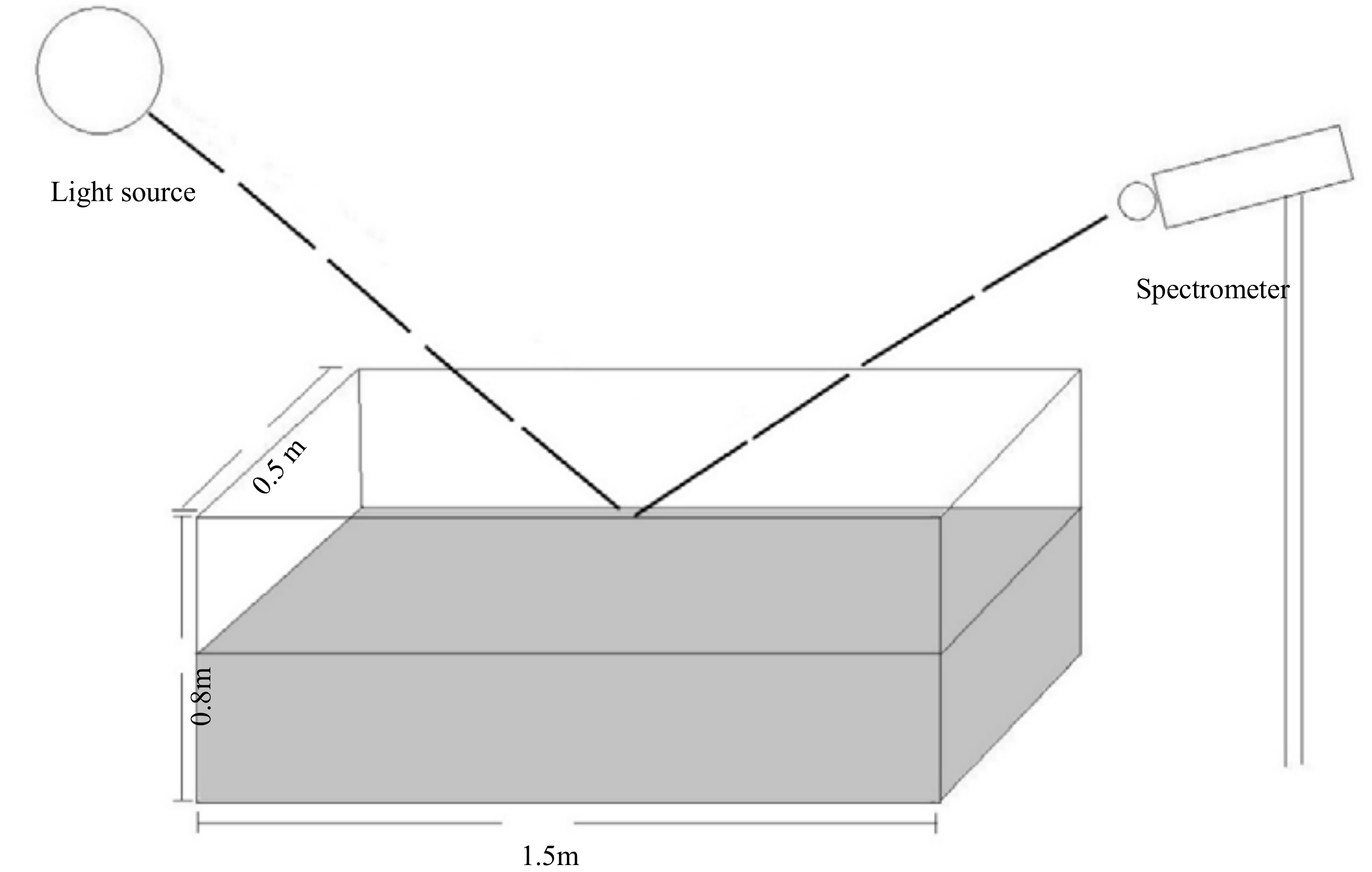
The sediment solution is placed in the box for measurement to imitate the influence of the environment surrounding the natural water landscape. The measurement system, as shown in (Figure 1), consists of a natural light source, a spectrometer and a water tank. The water tank used in the experiment is 1.5 m long, 0.5 m wide and 0.8 m high. The tank is covered by a black cloth to avoid the influence of the incident light. The bottom plate is measured with a blackboard and whiteboard to eliminate the influence of the baseplate on reflectivity. The reflectivity of the water body is measured by the full wavelength reflectance spectrometer (model: SOC710VP). Finally, the ash plate is used to calibrate it.
2.2. Data Collection
The sediment concentration under three different depths of water body, 20, 40 and 80 cm, are weighed using the quantitative Huang Taotu (sticky sediment) to study the influence of sediment concentration on the water landscape color under different water depths. The sediment concentrations of 10, 50, 100, 500 and 1000 mg/L are used as experimental samples in the container. All the samples are measured at the same time on the same day to objectively analyze the influence of the suspended sediment on the water landscape color, and the reflectivity of the clean water is measured as a contrast.
2.3. Establishment of Color Spectral Model for Water Landscape
2.3.1. CIE Chromaticity Calculation
According to the reflectance of the water body p(λ), the color of the water can be obtained using the CIE chroma calculation method. For color calculation, global research is more mature; this paper uses the color calculation standard of the CIE-XYZ system promulgated in 1931 by the International Photographic Commission (CIE) [27].
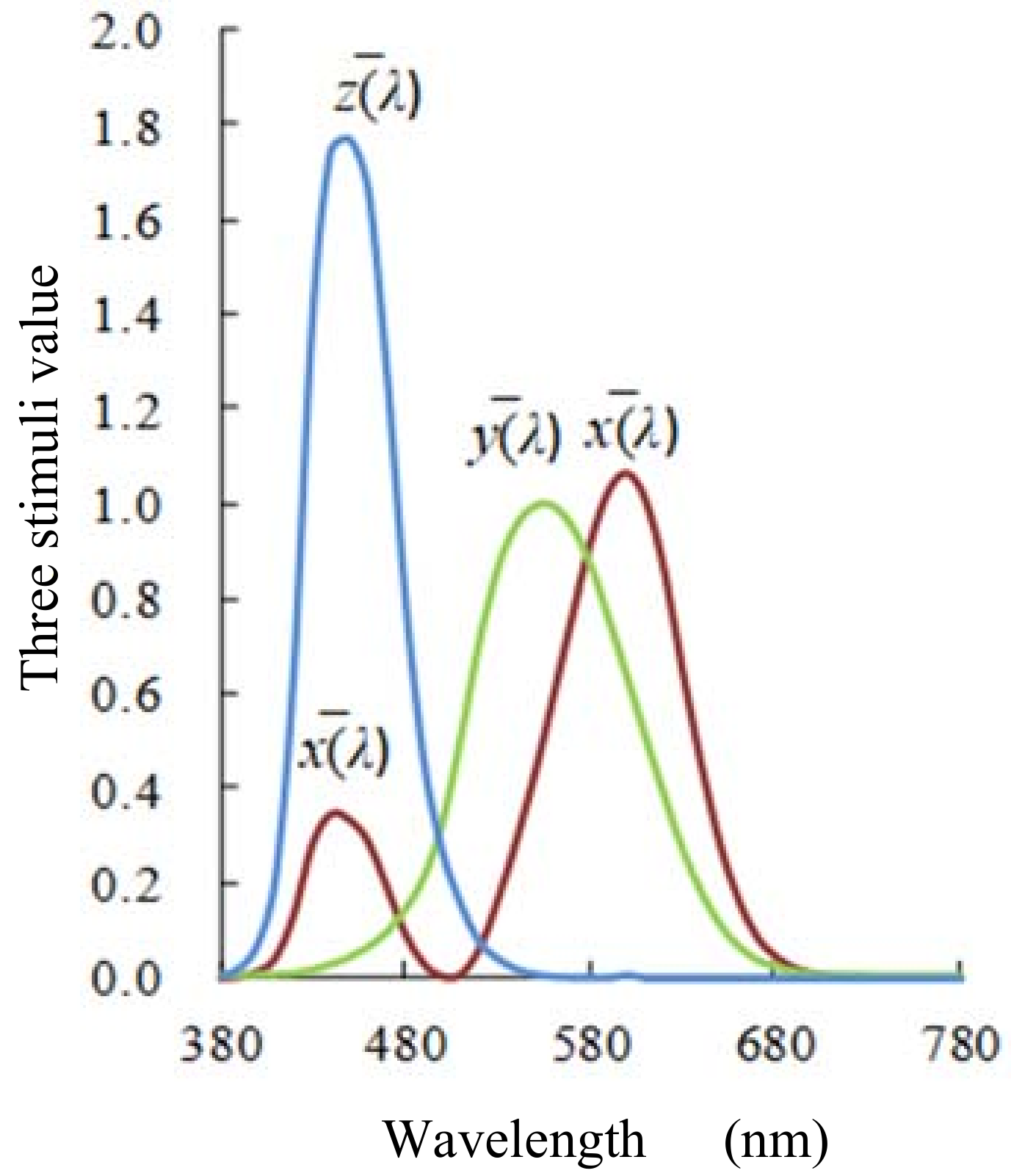
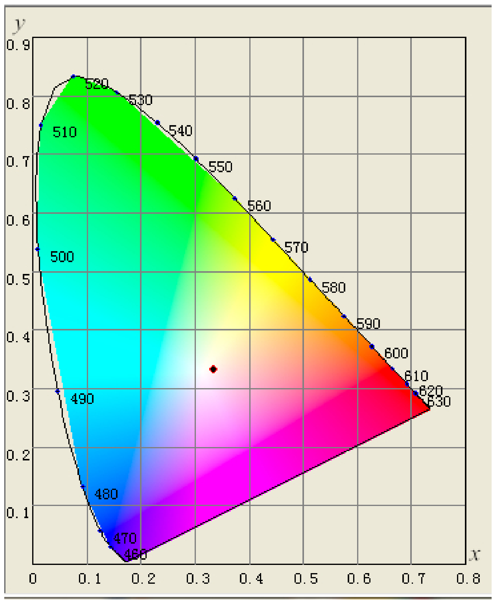
According to the characteristics of eye and color, any color that the eye can sense is based on the common effect of three kinds of pyramidal cells, that is, a comprehensive reflection of red, green and blue [28]. Almost any color can be mixed with red, green, and blue colors. In 1931, the International Lighting committee (CIE) proposed the “CIE-XYZ spectrum three stimulus system”. In this system, X represents imaginary red, Y represents imaginary green, and Z represents imaginary blue. CIE gives the three spectral stimulus curve of every equal-energy spectrum line, such as x(λ), y(λ) and z(λ), matching the red, green and blue primaries in the range of 380 to 780 nm, as shown in Figure 2. CIE has created the 1931CIE-XYZ chromaticity map, as shown in Figure 3. As shown in Figure 2 and Figure 3, the 1931CIE-XYZ system chromaticity graph looks like a horseshoe; thus, it is also known as the “horseshoe diagram”. A color map is a two-dimensional plane map with x as the horizontal coordinate and y as the longitudinal coordinate. Any point within its envelope represents a color. The landscape color of the light source or object can be determined as long as the coordinates of the light source or object on the color map, that is, the color coordinates (x, y), are obtained.
The 1931CIE-XYZ chromaticity system gives the calculation method for calculating the (x, y) of a light source or object. The three-stimulus values CIE, X, Y and Z caused by the color stimulus function (λ) can be expressed as
When calculating the three-stimulus values X, Y and Z, the summation formula is usually used instead of Type (1). Δλ is the range of each wavelength. A smaller value of Δλ, the calculation indicates more accurate calculation results. The general selection is expressed as
The X, Y and Z in Type (1) and (2) are the three stimulus values in the 1931CIE chroma system. x(λ), y(λ) and z(λ) are the spectral three irritation values of the 1931CIE chromaticity system, which can be obtained by the three-stimulus value table of the CIE standard chromaticity observation.
The k [27] in Type (1) and (2) is called the adjustment coefficient. For the illuminant or light source, its spectral radiative power is Фe(λ), and k is defined as:
The real meaning of Formula (3) is to adjust the Y of the illuminator or light source to 100, as follows:
After calculating the three stimulus values of X, Y and Z by Formula (2), the chromatic coordinates of objects can be obtained:
The chromatic coordinates (x, y) of the water body can be used to find the corresponding landscape color on the chromaticity map.
The color stimulus function (λi) is based on the inherent optical properties of the water body, and the water radiation value of each band is calculated. In this paper, the reflectance p(λi) of water directly received by hyperspectral instrument is used to replace the color stimulus function. In summary, the spectral model of the water landscape color consists of Equations (6)–(8):
In this paper, because of the accuracy of the instrument, takes 10 nm to establish a response relationship; because of more response relations, three special wavelengths, red, blue, and green, are used to establish relations.
2.3.2. Response Relationship between Reflectivity and Influence Factors of Water Body
In this paper, the relationship between water depth and sediment concentration in water and two factors affecting water landscape color is established using water quality factors that are easy to detect in water as indicators. A complete color spectral model of water landscape is constructed by establishing a response relationship between reflectance and the color of the water landscape and the CIE color computing model. According to observation and calculation, reflectance should be in accordance with water depth and sediment concentration:
p(λ) = f(d)k(c) + n(d)
p(λ)—reflectivity;
f(d)—the function equation related to the depth of water;
k(c)—a functional relationship containing various concentrations of water quality factors;
n(d)—reflectance function equation of clean water at different depths.
In summary, Formulae (7)–(9) constitute a complete color spectral calculation model of water landscape.
3. Main Influencing Factors of Water Landscape Color and Establishment of Evaluation Methods
In this paper, to establish the relationship between water depth and the concentration of water quality factors, the reflectance of p(λ) measured by instrument is calculated instead of the color stimulus value of (λ). Because the chromatic tricolor is red, green and blue, absorption and reflection of the three colors in the water is quite different. Therefore, the spectral reflectance variation trend of the water body under different sediment concentrations is measured by the full wavelength reflectance spectrometer. The influence of different water depth and sediment concentration on reflectance, peak value of reflectivity and chromatic tricolor reflectance of water body is studied to find the response relationship between reflectance and two water quality factors and establish a color of water landscape prediction method for sand-laden water bodies.
3.1. Influence of Sediment Concentration on Landscape Color of Water Body
Sediment is a kind of insoluble substance that widely exists in natural water body. Because of its own characteristics, sediment particles have different reflection effects on the light of different wavelengths. When mixed with certain sediments in water, the water body is yellow because of the absorption and reflection of sediment on different wavelengths, which seriously affects water landscape color. In this section, by measuring the variation trend of the reflectance spectra of different concentrations of suspended sediment in different depths of water, the influence of sediment concentration on the reflection spectrum of water body under different water depths is analyzed, and the quantitative response relationship between sediment concentration and water depth and reflectance is found.
3.1.1. Variation of the Reflectance of Suspended Sediment in Different Concentrations
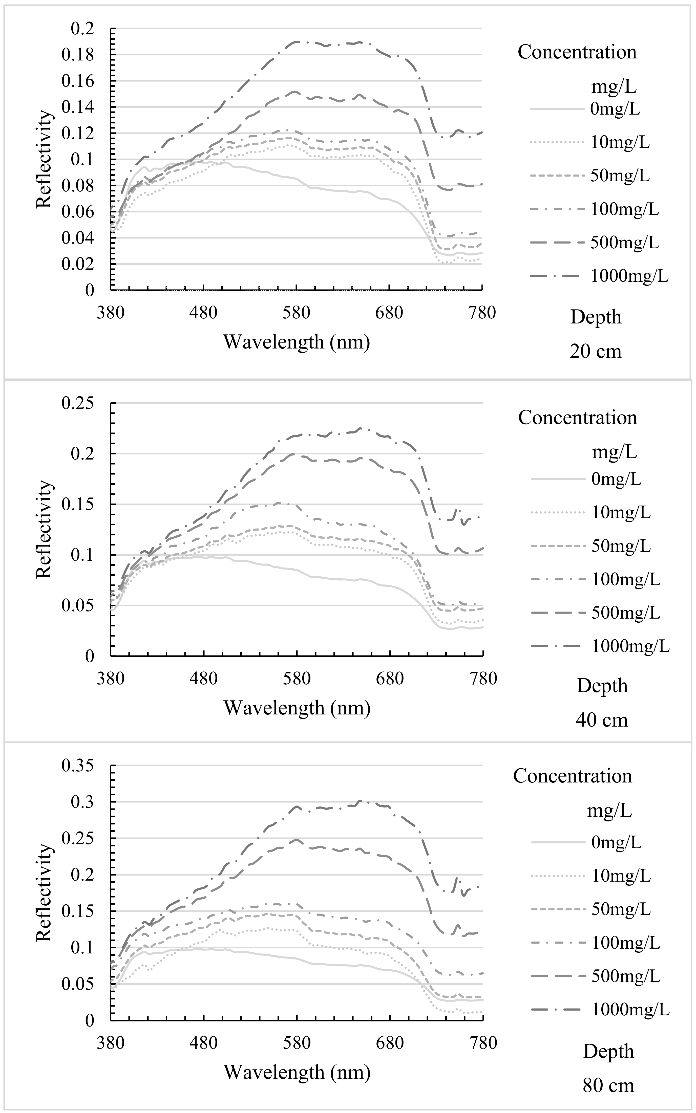
Table 1 is the statistical table of the peak value of the albedo of sediment suspension with different concentrations. From Table 1, it can be seen that the peak value of the reflectivity of the suspended sediment is in a different depth of water, and with an increase in the concentration of sediment, the peak wavelength of the reflectance increases, and the peak of the reflectance curve shifts to the right. Figure 4 is the change map of the reflectance curves of different concentration of suspended sediment in different depths of water. It can be seen that the reflectance wavelength curve of the sediment suspension is a bimodal pattern, which appears at 570 nm and 650 nm. Because of the optical characteristics of the sediment itself, the peak of the suspended sediment is not obvious, but shows a higher state between the wavelength range of 550~700 nm. In the three different water depth conditions, the reflectivity of the suspended sediment is increased with the increase of sediment concentration in the water body. This may be due to the increase of the water quality factor in the water body, which reduces the transmittance of the water body itself, and more light reflects in suspension, resulting in increased reflectivity of suspended sediment. In the same sediment concentration gradient, the reflectivity of the suspended sediment increases with the depth of the water body. This may be due to the increase in the depth of water, as the light can produce refraction in the increased water molecular level and thus increase the reflectivity of the water body.
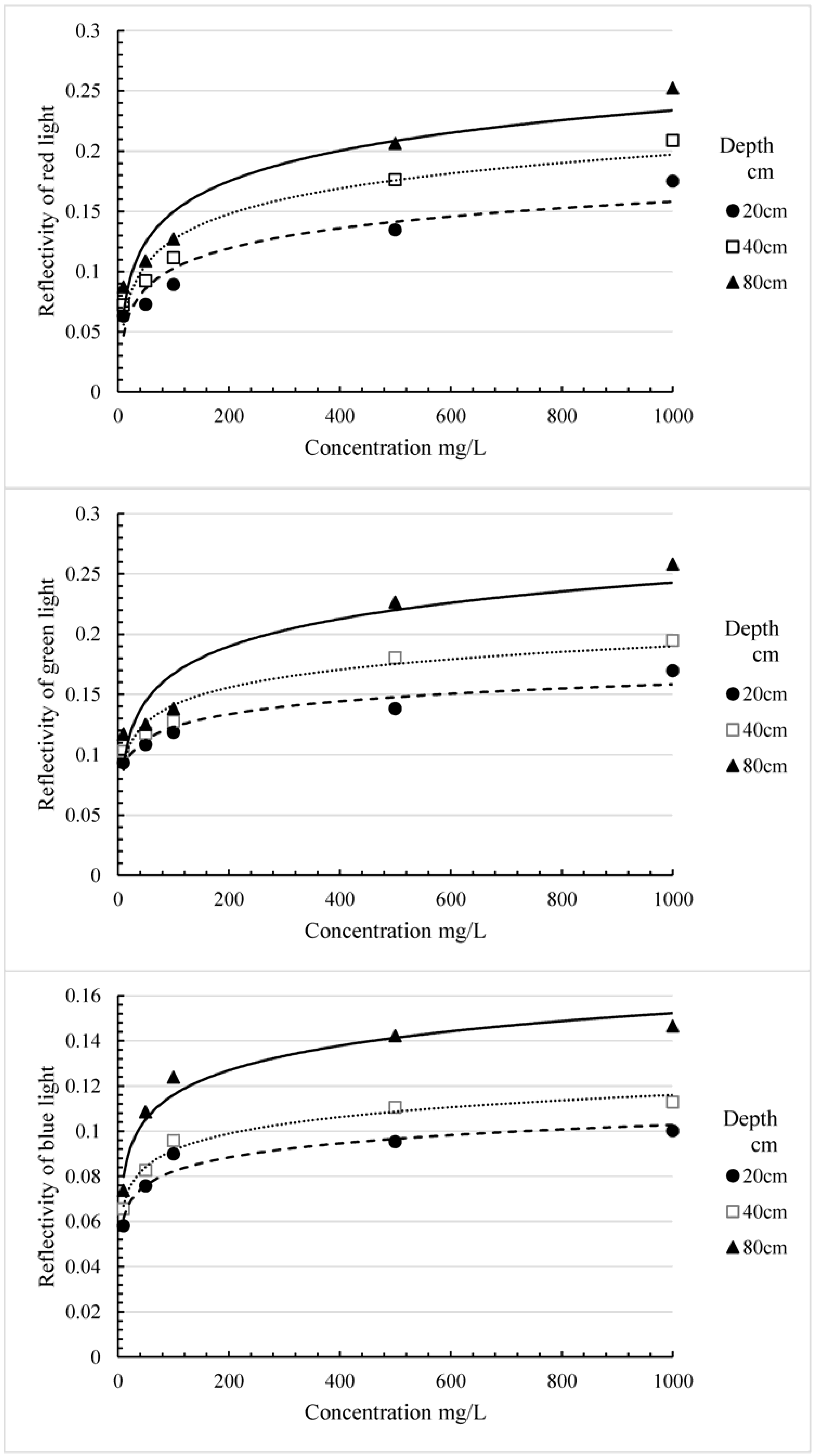
3.1.2. Reflectivity Response Relationship of Suspended Sediment to Trichromatic Wavelength
In Figure 5, the reflectance of red-light and green-light wavelength in sediment water is much higher than that of blue-light wavelength, indicating that most of the color of sediment water landscape is red and green. In Table 2, the coefficients of the logarithmic terms of red light and green light are much larger than those of blue light logarithmic terms, explaining that when the concentration of sediment in the water is increased, the reflectance of the wavelength of the chromatic tricolor light is on the rise, but the reflectance of the red and green light rises faster. It shows that when the concentration of the sediment in the water is increased, the red and green composition in the color of the water body is higher, which is in accordance with the actual image observed. When the sediment concentration in the water continues to increase, the rising rate of the reflectance of the red-light wavelength decreases. This is because the sediment concentration is low or zero, the red-light wavelength is longer, and it is not easy to scatter in the water body, which leads to the low reflectance of the red-light wavelength section in the water. While the sediment concentration is low or zero, because the green and blue wavelength is short, it is easy to scatter in the water, causing the green and blue wavelength reflectivity to be higher. When the sediment is added to the water, the change of the color system causes the reflectivity of the red and green light wavelength to rise rapidly, while the reflectivity of blue-light wavelength rises slowly. With the continuous increase of the sediment in the water body, the color system will not be greatly changed. As the sediment continues to increase, the refraction and scattering of light in the water body is reduced. When the concentration of the sediment is large enough, only the surface of the water body is reflected; thus, with the increase of sediment, the trend of the increase of chromatic tricolor reflectivity slows to final stability.
Table 2 is the chromatic tricolor reflectance curve equation of different water depths; it is fitted by reflectance of different sediment concentration under different water depth conditions by hyperspectral instrument. The regression curve of the reflectance of sediment suspension is a logarithmic equation, and the constant of the fitting formula is the reflectivity of chromatic tricolor in water.
3.1.3. The Response Relation between the Wavelength of Chromatic Tri Primary Color and the Reflectivity
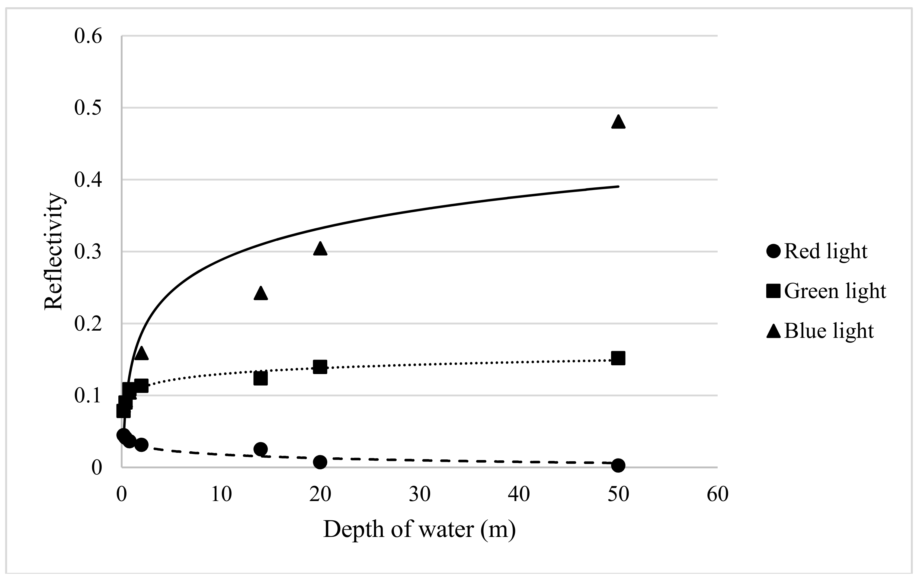
According to the reflectance response of the above water body to chromatic tricolor wavelength, the fitting equation of the variation of the reflectance of the sediment suspense with the concentration is a logarithmic equation. The different water depth has a different effect on the reflectance of different chromatic tricolor wavelengths, and it can be seen that it has the same influence on the change trend of reflectivity, with the change of the depth of water the only change of the coefficient. Therefore, the reflectance of suspended sediment should satisfy the following formula:
p(λ) = f(s)ln(c + 1) + n(λ)
p(λ)—The reflectivity of sediment suspension;
c—Sediment concentration;
n(λ)—Reflectivity of clear water.
Figure 6 shows the regression equation of the reflectance of chromatic light in the clean water with the depth of the water.
In the sediment suspension, f(s) has a different trend in the three primary colors. The experiment shows that the f(s) is related to the depth of the water body, and the data are fitted to the formula, which can be expressed as:
The response relationship between the reflectance of the suspended sediment and the depth of water and the concentration of sediment can be obtained by taking the fitting equation of f(s) and n(λ) of the chromatic tricolor as 10.
3.2. Experimental Verification of Landscape Color Prediction of Sediment Water
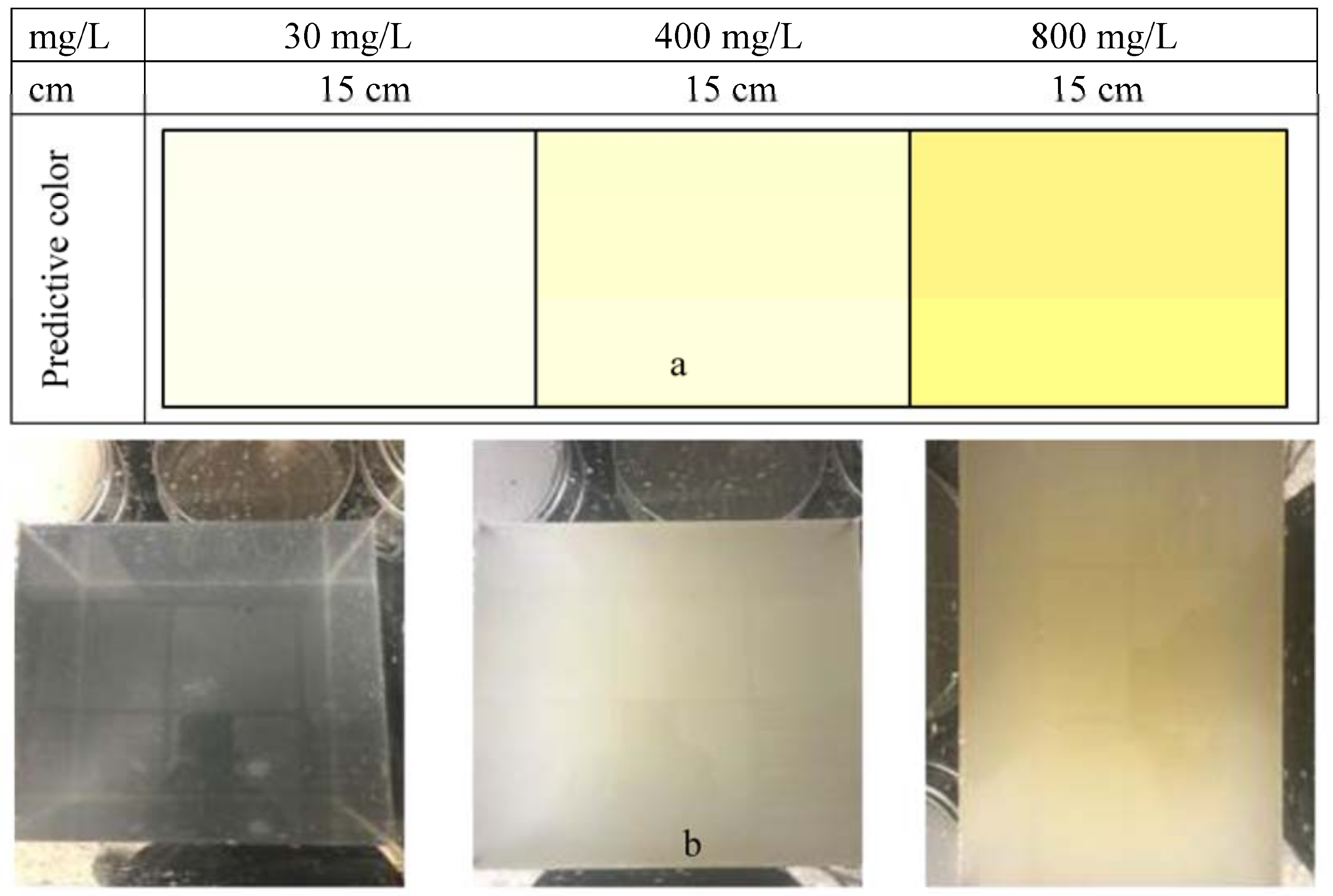
In the test, the depth of 15 cm and concentrations of 30 mg/L, 400 mg/L and 800 mg/L, were not selected in the sediment experiment. If the water landscape color calculated according to these concentrations accords with the actual pictures, it could be proved that the color calculated by the color spectral model of the water landscape was correct and has some practical value. Therefore, these concentrations were selected as the depth and concentration of the test, expressed as follows:
Then, Formulae (11) and (13) were taken into the same depth gradient, and the fitting Equation (10) of the suspended sediment reflectivity varied with the concentration; its expression is:
Then, the sediment concentration 30 mg/L, 400 mg/L and 800 mg/L in the experimental test were brought into Type (14), and the depth of the sediment in the 15 cm water body was obtained. The chromatic tricolor reflectance of three different concentrations of suspended sediment is shown in Table 3.
Three different concentrations of chromatic tricolor reflectance of sediment suspended in the depth of 15 cm water, such as Table 3, were added to Equations (7) and (8), and the chromaticity coordinates of water body with sediment concentration in 15 cm depth obtained, as shown in Table 4.
Figure 7a is the result of the calculation of water landscape color under different sediment concentrations calculated according to the variation of sediment concentration in Table 4. Figure 7b is a picture of the water landscape color under different sediment concentrations.
From Figure 7a,b, it can be seen that the landscape color prediction of sediment water body basically conforms to the change of water landscape color caused by the change of sediment concentration, and water landscape color is mainly influenced by the change of sediment concentration in the case of less depth change. The color map of the water landscape color calculated by sediment concentration is consistent with the color changes of actual photographs, and the trend of color depth is consistent. The map shows that the water color of the suspended sediment is basically in line with the actual change rule, with a change in sediment concentration. This map proved that the reflectivity response relation which was established before is effective and practical.
3.3. Establishment of Evaluation Method for Influence of Sediment on Water Landscape Color
In natural water, the landscape color of the water body is mainly determined by the depth of water body and the concentration of water quality factor in the water body. The influence of water depth on the landscape color of the target water body should be determined first. After determining the depth of the water body, the concentration of the water quality factor in the water body is measured, and the reflectance p(λ) of the water containing the sediment factor is obtained in the reflectance fitting equation of the natural water body at the depth of the water body, Equation (10). Then, the reflectance p(λ) is calculated, using Equations (7) and (8) to obtain the chromaticity coordinates (x, y) of different water quality factors under this depth gradient. The concept of absolute value of chromaticity coordinates is introduced here. The chromaticity coordinates of the water landscape color of natural water body, which is caused by the change of water quality factor concentration, are compared with the chromaticity coordinates of the original water landscape color of the natural water body, and the difference is used to make a significant impact assessment on the water landscape color. The chromaticity reflectance of natural water is calculated according to the albedo variation of the chromatic tricolor wavelength, and the chromaticity coordinate values (x0, y0) of the natural water body are calculated according to Formulae (7) and (8). Finally, the chromaticity coordinates (x1, y1) of the target natural water under the influence of water quality factor concentration are calculated as a benchmark for evaluation.
In the water landscape color evaluation standard, the color change of the chromaticity diagram of the water body color is diverged from the middle to the surrounding area; thus, the chromaticity coordinates values of the predictive target water body subtract the original chromaticity coordinate values of the target natural water body to establish the color judgment relation of the water landscape; its expression is:
(x1 − x0)2 + (y1 − y0)2 = r2
x1, y1—Target natural water body prediction of chromaticity coordinates;
x0, y0—The initial chromaticity coordinate values of the target natural water body;
r—Determination of the significant influence of color of water landscape.
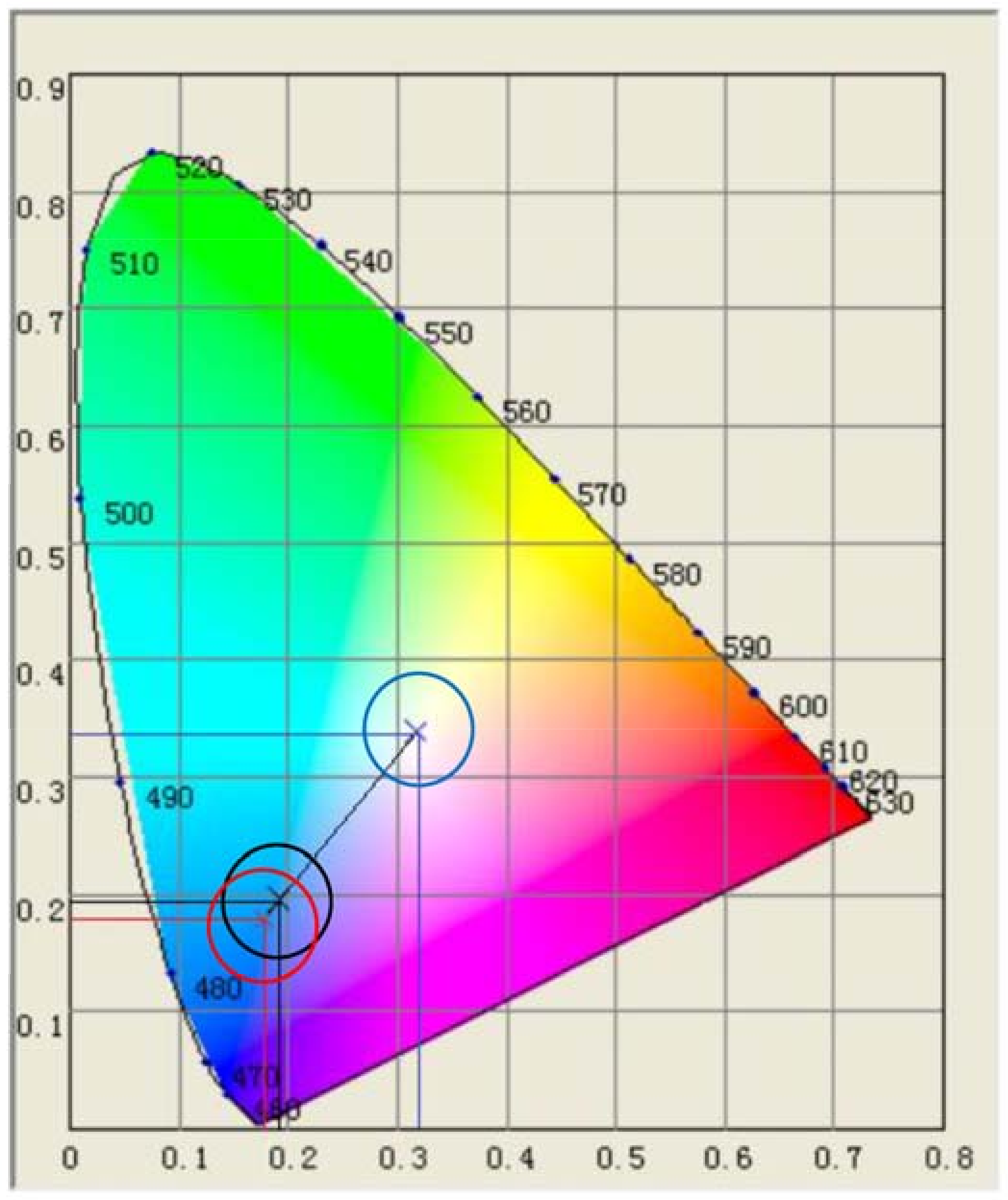
As shown in Figure 8, at three different depths with the initial state of clean water, when
defines the water landscape color, there is a significant difference.
(x1 − x0)2 + (y1 − y0)2 > r2
Additionally, in three different water depths, when
the water landscape color is defined as having no significant difference.
(x1 − x0)2 + (y1 − y0)2 < r2
The color change in the chromaticity diagram is determined by the position of the chromaticity coordinates, and the change in the chromaticity coordinates can be expressed by a fixed value, such as the three circles in Figure 8. According to the actual observation, when r is greater than 0.05, that is, beyond the circle, it is defined that under the concentration of the water quality factor, the landscape color of the water body is significantly different; when r is less than 0.05, it is defined in the circle as having no significant difference in the landscape color of the water quality factor.
3.4. Landscape Color Evaluation of a Natural Water Body in a High Mountain Lake
This section focuses on lake sediment flow into the lake as the research objective to study the applicability and prediction function of the water landscape color spectrum model to water landscape color under different sediment concentration scenarios. The sediment inlet is located in the area of Tibet and Gongga. The lake is a plateau lake with a high salinity. The area is 675 km, and the lake is 4441 m above sea level. The average depth of the lake is approximately 40 m. As the power station uses the excess electricity load during the low load period to extract water from Yajiang lake to energy storage in the lake, it leads to sediment inflow into the lake. Maximum pumping capacity of power station 8 m3/s. The median particle size of sediment is d50 = 7.65 µm. The water body is clean, and the sediment content is small when no sediment enters into the flow. The sediment color is yellow brown when the sediment enters the flow, and the sediment content is based on the monitoring results of the natural water body of the mountain lake [29]. The landscape color of the sediment water flow in the lake is simulated and predicted by using the spectral model of the landscape color of the suspended sediment water. The applicability of the spectral model method is analyzed and discussed.
Because the water quality is good and the water body clean when no sediment is in flow, pure sea water is chosen as the background water body, and the depth reflectance fitting formula of pure sea water is used to calculate the water body. However, the composition and content of salt in the lake water and the composition and content of salt in pure seawater are not considered in the calculation.
Table 5 is a summary table of the predictive chromaticity coordinates of a mountain lake with different sediment concentrations. The average water depth in the reservoir area is 40 m. When the depth of water is 40 m, the depth of water is taken into Formula (10); its expression is:
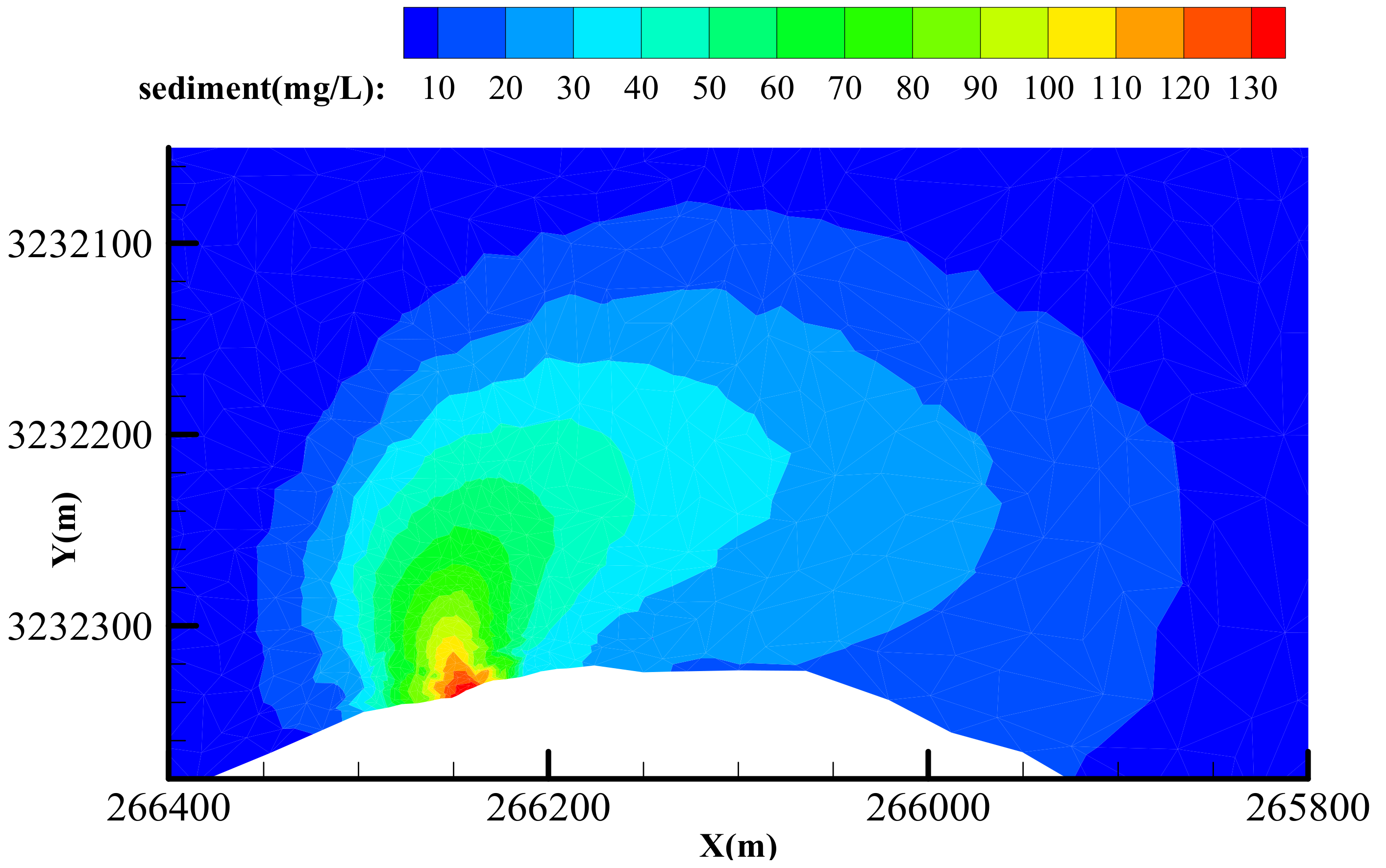
According to the sediment distribution of a lake’s sediment-laden discharge in the area nearby, the sediment concentration gradient distribution of a lake’s sediment-laden water body is determined (Figure 9). Then, the sediment content of the lake was brought into Formulae (7) and (8) to get the chromatic coordinate distribution corresponding to the sediment distribution in the water body (Table 5). The chromatic coordinates of different sediment concentrations were considered (15) for evaluation.
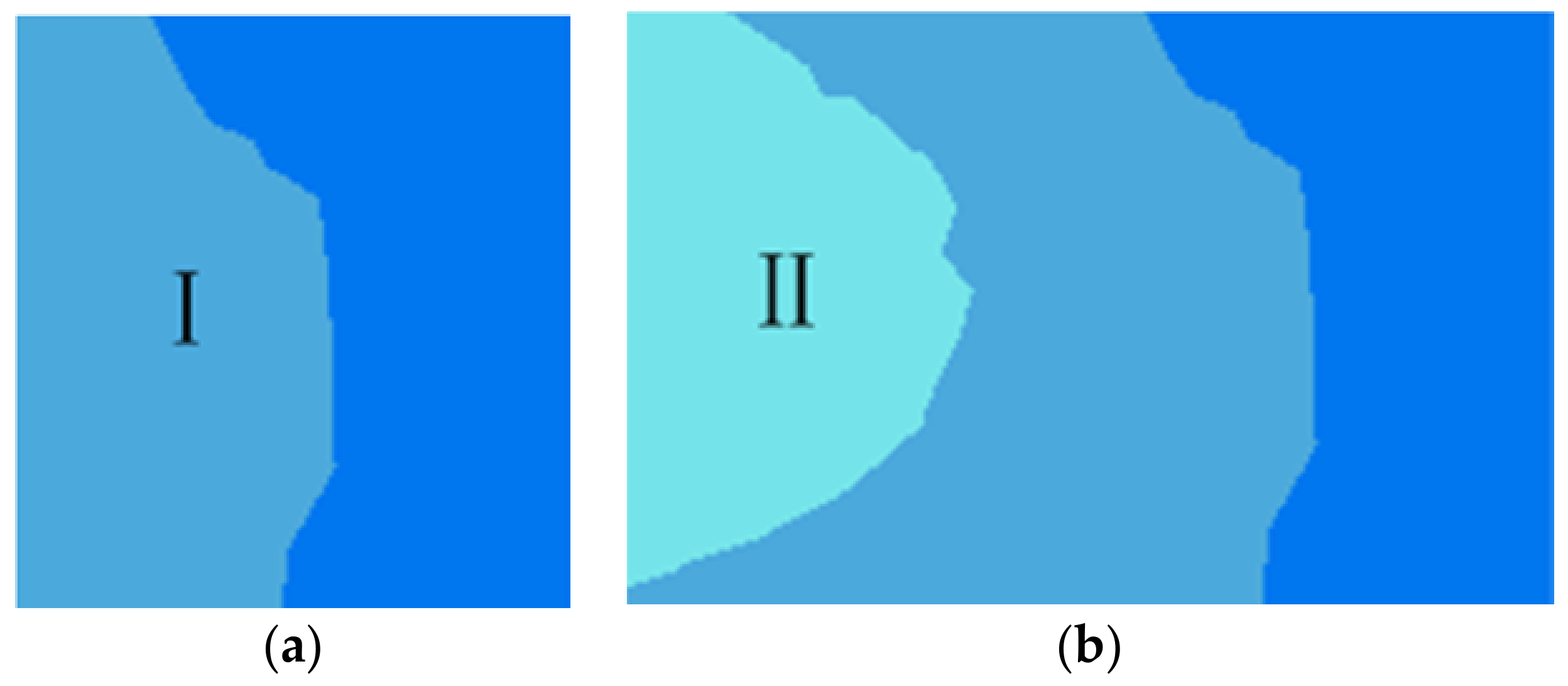
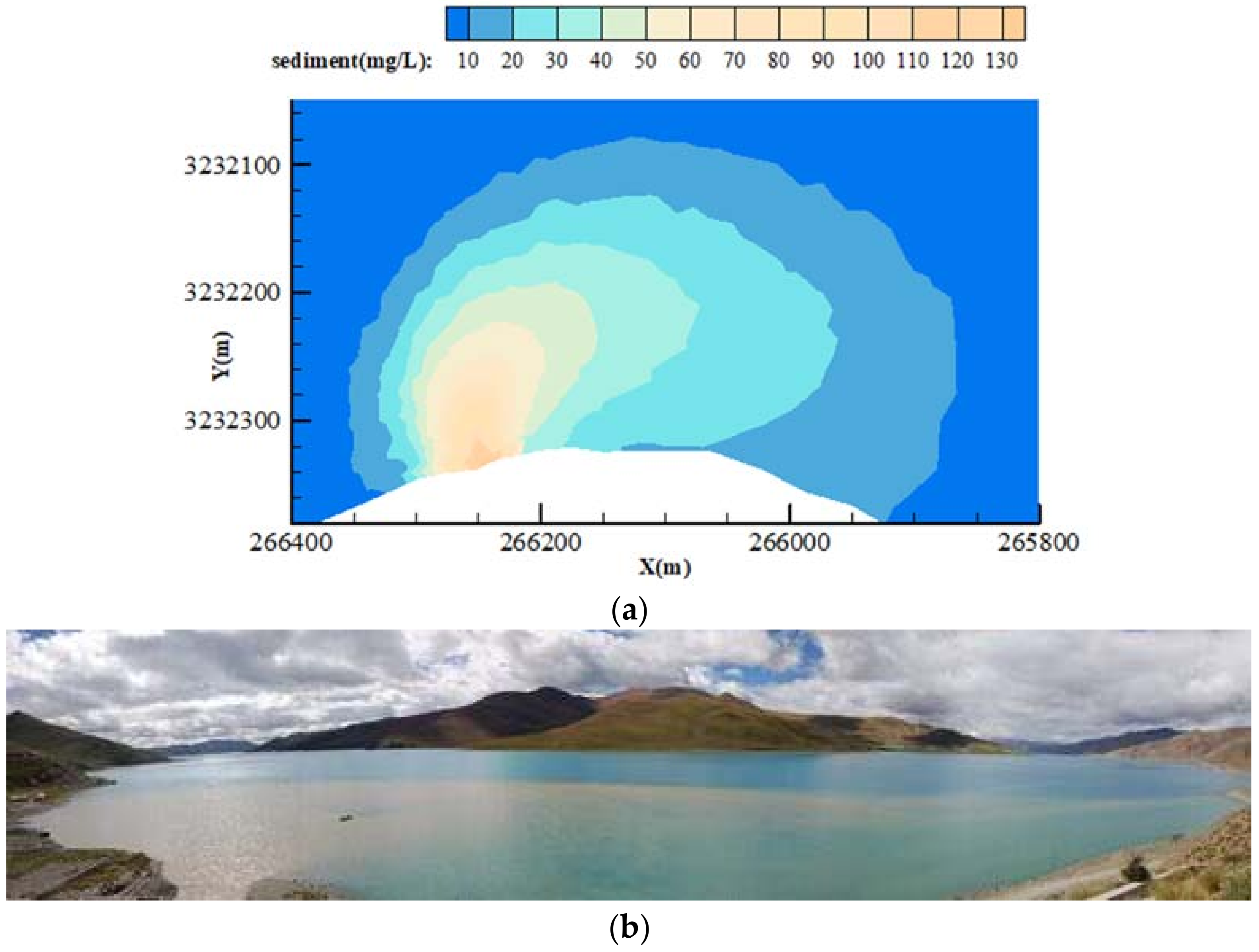
From the water landscape color evaluation method, it is found that the judgment value of the significant influence of sediment in water body on the water landscape color is 0.05. When the sediment concentration is less than 10 mg/L, as shown in Figure 10a, there is a difference in color between sand area I and pure seawater, but the overall color is unchanged. r is 0.037, which is less than the r = 0.05 value of water landscape color, and there is no significant difference in the color of the water landscape. When the concentration of sediment is between 10 mg/L and 20 mg/L, such as Figure 10b, the color of Region II is obviously different from that of pure sea water, and the whole color system changes. Because of the influence of depth on water landscape color Alpine lakes, water landscape color changes little when the sediment concentration is relatively small, which is similar to the actual river; Region II changes from a blue system to a yellow system. r is 0.115, which is larger than the r = 0.05 value of water landscape color, and there is a significant difference in the color of the water landscape. Because of the continuous increase of sediment concentration, the influence of water landscape color gradually increases, resulting in water landscape color, similar to the actual river situation. When the sediment concentration is greater than 30 mg/L, r is greater than the water landscape color, which has a significant impact on the determination value of 0.05; therefore, a higher concentration of sediment causes a significant difference in the landscape color of the lake. Figure 11a is a landscape color prediction map of the water flow into a high mountain lake. It can be seen from the map (Figure 11a) that the color change of the water landscape does not vary much from 0 mg/L to 10 mg/L, and the basic color system is not changed. When the sediment concentration increases from 10 mg/L to 20 mg/L, the color of the water landscape is obviously yellow, and the sediment has a significant effect on the color of the water landscape. The picture of water landscape color flowing into the lake with the sediment-laden flow of a high mountain lake is shown in Figure 11b. The sediment-laden water diffuses from the point source and forms a pollution circle as the sediment continues to diffuse. The color depth gradually decreases from around the point source and is consistent with the color change of water landscape color picture (Figure 10) calculated by the spectral model. This indicates that the prediction picture basically reflects the trend of the water landscape color. This comparison proves that the evaluation method of water landscape color has certain application values in natural waters.
4. Conclusions
Through the simulation experiment, the influence pattern of the sediment water quality factor on the reflectance of water body is studied. The formula for predicting the reflectance of the sediment water body is established by measuring the reflectance of the sediment with different concentrations at different depths. Then, combined with the CIE chromaticity calculation method, the spectral model of water landscape color is established. Accordingly, the color coordinates of water landscape color can be calculated, contributing to the quantitative evaluation of water color of the different color systems at different water depths.
Through the verification test by spectral model of water landscape color, the water color calculated by the model established in this report, the result is basically consistent with the actual color of the water body, demonstrating that the calculation formula of water body reflectance and the color spectrum model of the water landscape can be applied to calculate the landscape color of natural water body with different sediment concentrations.
According to the variation of the sediment content in a lake, the color of the water body with different concentration gradients was calculated. The color change trend, which was ascertained from the landscape color prediction map of the Alpine lake, is similar to the actual observation, illustrating that the color spectral model of water landscape can be used to calculate the color of natural water under the influence of sediment. Furthermore, based on the chromaticity coordinates, the evaluation results of the color difference of the water landscape can also reflect the observation results accurately, which demonstrates the accuracy and reliability of the color spectral model.
Some traditional remote sensing methods can also be applied in assessing the pollutant influence on the water quality, but these methods are only based on the polluted water, and lack a prediction function for water landscape color. Therefore, in this research, we established the relationship between water quality factors and water landscape color in lakes by hyperspectral instruments, so we can predict the water landscape color and then apply this when evaluating the pollutant influence of sediment discharge projects based on water quality factors. However, while this new method can quantify how the sediment factor affects water landscape color, the question of how other water quality factors (such as heavy metal ion and algae) influence water color remains unanswered. Therefore, more research is needed to quantify the relationship of water landscape color and various water quality factors, thus contributing to a more complete and reliable water body landscape color evaluation system.
Author Contributions
Data curation and Writing—original draft, M.Y.; Software and Writing—review & editing, X.P.; Investigation and Methodology, R.L.; Project administration, W.T.; Funding acquisition, J.L.
Acknowledgments
This research was supported by the National Key R and D Program of China (Grant No. 2016YFC0401710) and National Natural Science Foundation of China (91547211). Thanks to Sichuan EIA for its project funding support. Thanks to postgraduate support from State Key Laboratory of Hydraulics and Mountain River Engineering.
Conflicts of Interest
The authors declare no conflicts of interest.
References
- Smith, S.V.; Renwick, W.H.; Bartley, J.D.; Buddemeier, R.W. Distribution and significance of small, artificial water bodies across the United States landscape. Sci. Total Environ. 2002, 299, 21–36. [Google Scholar] [CrossRef]
- Zhao, S.; Fang, J.; Ji, W.; Tang, Z. Lake restoration from impoldering: impact of land conversion on riparian landscape in Honghu Lake area, Central Yangtze. Agric. Ecosyst. Environ. 2003, 95, 111–118. [Google Scholar] [CrossRef] [Green Version]
- Wang, H.L. Approach on the quality standard for reuse of reclaimed water in scenic waters. China Water Wastewater 2001, 17, 31–35. [Google Scholar]
- Richardson, C.J.; Flanagan, N.E.; Ho, M.; Pahl, J.W. Integrated stream and wetland restoration: A watershed approach to improved water quality on the landscape. Ecol. Eng. 2011, 37, 25–39. [Google Scholar] [CrossRef] [Green Version]
- Wang, F.; Huang, Y.; Pan, Y.; Wang, J.; Wu, Q.Y. Application for a Method of Evaluating the Apparent Quality of Urban Scenic Water. Environ. Sci. Technol. 2017, 2, 186–189. [Google Scholar]
- Na, S.; Yang, H.; Li, X.Y. Identification of pollutant with different apparent characteristics and types of pollution in urban water. Water Resour. Prot. 2015. [Google Scholar]
- Wang, F.; LI, H.; Ai, N.; Lin, X.; Jing, D. Fractals and selforganizations of motion of water flow and sediment as well as fluvial PROCESSES. Explor. Nat. 1999, 3, 55–61. [Google Scholar]
- Cai, S.T. Sedimentation motion of sand particles in water (II) the effect of time factor. Acta Phys. Sin. 1956, 5, 409–418. [Google Scholar]
- Water Quality—Examination and Determination of Colour; ISO 7887-1985; International Organization for Standardization: Geneva, Switzerland, 1985; pp. 1–7.
- State Environmental Protection Administration. Determination of Water Color. GB/T 11903-1989; China Standard Publishing House: Beijing, China, 1989; pp. 1–3. [Google Scholar]
- Yu, P.; Shen, W.; Huang, J.; Xu, B. Determination of water colority by spectrophotometry in visible spectrum. Opt. Tech. 2011, 37, 551–555. [Google Scholar]
- Zhao, T.C. Light radiation properties of suspended sediments in the waters. Mar. Sci. Bull. 1983, 4, 42–53. [Google Scholar]
- Liu, L.M.; Zhu, J.D. Preliminary Study on Trend of Ocean Color Sensor Development. Remote Sens. Inf. 2011, 28, 111–119. [Google Scholar]
- Xu, X.R. Remote Sensing Physics; Peking University Press: Beijing, China, 2006. [Google Scholar]
- Xi, C.W.; Ying, Z.Q.; Zhong, Y.Y. Principal Component Analysis for Ocean Color Remote Sensing in South China Sea. J. Remote Sens. 1999, 2, 19–32. [Google Scholar]
- Wang, S.Y.; Liu, C.; Yang, S.Z. Multi-source RS data based analysis on regional eco-landscape change before and after construction of Xixiayuan Reservoir. Water Resour. Hydropower Eng. 2011, 11, 22–25. [Google Scholar]
- Ma, R.H.; Tang, J.W. Remote sensing parameters acquisition and algorithm analysis of lake color. Adv. Water Sci. 2006, 17, 720–726. [Google Scholar]
- Liew, S.C.; Lu, X.X.; Chen, P.; Zhou, Y. Remote Sensing Estimation of Suspended Sediment Concentrations in Highly Turbid Inland River Waters: An Example from the Lower Jinsha Tributary, Yunnan, China. J. Mt. Res. 2003, 21, 378–379. [Google Scholar]
- Yan, H.; Yao, Z.; Huang, H.; Jiang, D.; Dong, X.; Duan, R.; Zhang, Y. Water quality and light absorption attributes of glacial lakes in Mount Qomolangma region. J. Geogr. Sci. 2013, 23, 860–870. [Google Scholar] [CrossRef]
- Gong, C.L.; Yin, Q.; Kuang, D.B. Correlations between Water Quality Indexes and Reflectance Spectra of Huangpujiang River. J. Remote Sens. 2006, 10, 910–916. [Google Scholar]
- Chen, Z.; Hu, C.; Muller-Karger, F. Monitoring turbidity in Tampa Bay using MODIS/Aqua 250-m imagery. Remote Sens. Environ. 2007, 109, 207–220. [Google Scholar] [CrossRef]
- Doxaran, D.; Cherukuru, N.; Lavender, S.J. Apparent and inherent optical properties of turbid estuarine waters: Measurements, empirical quantification relationships, and modeling. Appl. Opt. 2006, 45, 2310–2324. [Google Scholar] [CrossRef] [PubMed]
- Qi, Y.Q.; Duan, Z.Y.; Lv, X. Research of Cotton Canopy Characteristic Information by Hyperspectral Remote Sensing Data. In Proceedings of the 2013 8th International Conference on Computer Science & Education, Colombo, Sri Lanka, 26–28 April 2013. [Google Scholar]
- Kallio, K.; Kutser, T.; Hannonen, T.; Koponen, S.; Pulliainen, J.; Vepsäläinen, J.; Pyhälahti, T. Retrieval of water quality from airborne imaging spectrometry of various lake types in different seasons. Sci. Total Environ. 2001, 268, 59–77. [Google Scholar] [CrossRef]
- Koponen, S.; Pulliainen, J.; Servomaa, H.; Zhang, Y.; Hallikainen, M.; Kallio, K.; Vepsäläinen, J.; Pyhälahti, T.; Hannonen, T. Analysis on the feasibility of multi-source remote sensing observations for chl-a monitoring in Finnish lakes. Sci. Total Environ. 2001, 268, 95–106. [Google Scholar] [CrossRef]
- Sun, D.Y.; Li, Y.M.; Wang, Q.; Le, C.F.; Huang, C.C.; Shi, K.; Wang, L.Z. Study on remote sensing estimation of suspended matter concentrations based on in situ hyperspectral data in lake tai waters. J. Infrared Millim. Waves 2009, 28, 124–128. [Google Scholar] [CrossRef]
- CIE. Commission Internationale de l’Eclairage Proceedings, 1931; Cambridge University Press: Cambridge, UK, 1932. [Google Scholar]
- Yang, Z.G. Eyes and Color; Print World: Hong Kong, China, 2004; pp. 6–7. [Google Scholar]
- Yu, Y.; Pu, X.; Li, R.; Jiang, H.; Li, Y. A study on organoleptic chromaticity-based quantitative assessment method for landscape quality of sandy water. J. China Inst. Water Resour. Hydropower Res. 2015, 13, 414–420. [Google Scholar]
Figure 1.
Color spectrum measurement system for water landscape. Light source is the natural light source of the sun. Spectrometer is a hyperspectral instrument.
Figure 1.
Color spectrum measurement system for water landscape. Light source is the natural light source of the sun. Spectrometer is a hyperspectral instrument.

Figure 2.
1931CIE-XYZ standard x(λ), y(λ) and z(λ). The three curves represent the radiation value of chromatic tricolor in the D50 [23] light source with the wavelength of visible light. The three stimuli output a value specified by CIE, the abscissa is the change of wavelength, and the unit is nm.

Figure 3.
1931CIE-XYZ system color map spectrum three stimulus value. The area of the horseshoe is the area for calculating the color distribution of color. The value of the boundary of the horseshoe diagram is the color represented by the spectrum of different wavelengths.
Figure 3.
1931CIE-XYZ system color map spectrum three stimulus value. The area of the horseshoe is the area for calculating the color distribution of color. The value of the boundary of the horseshoe diagram is the color represented by the spectrum of different wavelengths.

Figure 4.
Reflectivity curves of different experimental depths for different sediment concentrations. Depth is the change of water depth. Concentration is the change of sediment concentration. Wavelength is wavelength variation of visible light.
Figure 4.
Reflectivity curves of different experimental depths for different sediment concentrations. Depth is the change of water depth. Concentration is the change of sediment concentration. Wavelength is wavelength variation of visible light.

Figure 5.
Curves of chromatic light tricolor reflectance with sediment concentration at different depths of water.
Figure 5.
Curves of chromatic light tricolor reflectance with sediment concentration at different depths of water.

Figure 6.
The reflectance of color and trichromatic wavelength varies with the water depth.

Figure 7.
(a) Calculation results of water landscape color under different sediment concentrations picture (experimental depth 15 cm). (b) Real picture of water landscape color under different sediment concentrations (experimental depth 15 cm).
Figure 7.
(a) Calculation results of water landscape color under different sediment concentrations picture (experimental depth 15 cm). (b) Real picture of water landscape color under different sediment concentrations (experimental depth 15 cm).

Figure 8.
Clean water at different depths on the chromaticity diagram coordinate position diagram.

Figure 9.
Sediment distribution by sand-laden discharge in an area near the lake.

Figure 10.
Contrast diagram of the significant color difference of water landscape. (a) indicates that there is no significant difference between the Ⅰ regions and the sea water, (b) indicates that there is a significant difference between the 2 regions and the sea water.
Figure 10.
Contrast diagram of the significant color difference of water landscape. (a) indicates that there is no significant difference between the Ⅰ regions and the sea water, (b) indicates that there is a significant difference between the 2 regions and the sea water.

Figure 11.
Water landscape color prediction map and real map of Alpine lakes. The sediment inlet is located in the area of Tibet and Gongga. (a) is a picture of prediction of water landscape color in a high mountain lake with sediment-laden discharge. (b) is a real picture of the water landscape color of water flowing into a high mountain lake.


Table 1.
In three different water depth conditions, statistical table of peak wavelength corresponding to the reflectance of suspended sediment in different concentrations.
Table 1.
In three different water depth conditions, statistical table of peak wavelength corresponding to the reflectance of suspended sediment in different concentrations.
| Depth of Water | Concentration of Suspended Sediment | |||||
|---|---|---|---|---|---|---|
| 0 mg/L | 10 mg/L | 50 mg/L | 100 mg/L | 500 mg/L | 1000 mg/L | |
| 20 cm | 472.36 | 569.75 | 569.75 | 569.75 | 580.09 | 580.09 |
| 40 cm | 472.36 | 559.44 | 559.44 | 559.44 | 574.92 | 647.65 |
| 80 cm | 472.36 | 549.13 | 549.13 | 549.13 | 580.09 | 647.65 |
Table 2.
Reflectance equation of chromatic tricolor at different depths of water. R2 is the correlation coefficient.
Table 2.
Reflectance equation of chromatic tricolor at different depths of water. R2 is the correlation coefficient.
| Chromatic Tricolor | Depth of Water cm | Reflectivity Curve Equation | R2 |
|---|---|---|---|
| Red light | 20 | p(λ) = 0.02564ln(c + 1) + 0.04472 | 0.7973 |
| 40 | p(λ) = 0.02623ln(c + 1) + 0.04123 | 0.8376 | |
| 80 | p(λ) = 0.02714ln(c + 1) + 0.03634 | 0.8098 | |
| Green light | 20 | p(λ) = 0.01484ln(c + 1) + 0.07842 | 0.8841 |
| 40 | p(λ) = 0.01564ln(c + 1) + 0.09030 | 0.8516 | |
| 80 | p(λ) = 0.01714ln(c + 1) + 0.10863 | 0.7736 | |
| Blue light | 20 | p(λ) = 0.00873ln(c + 1) + 0.08584 | 0.9569 |
| 40 | p(λ) = 0.00923ln(c + 1) + 0.09321 | 0.9672 | |
| 80 | p(λ) = 0.01002ln(c + 1) + 0.10421 | 0.9221 |
Table 3.
Verification of reflectance of different concentrations of suspended sediment by trichromatic color (experimental depth 15 cm).
Table 3.
Verification of reflectance of different concentrations of suspended sediment by trichromatic color (experimental depth 15 cm).
| Color Trichromatic Reflectivity | Sediment Concentration mg/L | ||
|---|---|---|---|
| 30 mg/L | 400 mg/L | 800 mg/L | |
| Red color light | 0.1314 | 0.1971 | 0.2149 |
| Green color light | 0.1389 | 0.1755 | 0.1854 |
| Blue color light | 0.0939 | 0.1154 | 0.1211 |
Table 4.
Verification of chromatic coordinates of 15 cm water depth with changes in sediment concentration.
Table 4.
Verification of chromatic coordinates of 15 cm water depth with changes in sediment concentration.
| Chromaticity Coordinates | Sediment Concentration mg/L | ||
|---|---|---|---|
| 30 mg/L | 400 mg/L | 800 mg/L | |
| x | 0.315 | 0.338 | 0.353 |
| y | 0.363 | 0.377 | 0.385 |
Table 5.
Summary of chromatic coordinates prediction for a mountain lake with different sediment concentration changes.
Table 5.
Summary of chromatic coordinates prediction for a mountain lake with different sediment concentration changes.
| Chromaticity Coordinates | Sediment Concentration mg/L | ||||||
|---|---|---|---|---|---|---|---|
| 0 | 10 | 20 | 30 | 40 | 50 | 60 | |
| x | 0.161 | 0.179 | 0.208 | 0.231 | 0.270 | 0.339 | 0.350 |
| y | 0.146 | 0.179 | 0.251 | 0.297 | 0.355 | 0.407 | 0.409 |
| Chromaticity Coordinates | Sediment Concentration mg/L | ||||||
| 70 | 80 | 90 | 100 | 110 | 120 | 130 | |
| x | 0.368 | 0.374 | 0.384 | 0.387 | 0.390 | 0.395 | 0.398 |
| y | 0.411 | 0.410 | 0.409 | 0.403 | 0.401 | 0.400 | 0.398 |
© 2018 by the authors. Licensee MDPI, Basel, Switzerland. This article is an open access article distributed under the terms and conditions of the Creative Commons Attribution (CC BY) license (http://creativecommons.org/licenses/by/4.0/).
Share and Cite
MDPI and ACS Style
Ye, M.; Li, R.; Tu, W.; Liao, J.; Pu, X. Quantitative Evaluation Method for Landscape Color of Water with Suspended Sediment. Water 2018, 10, 1042. https://doi.org/10.3390/w10081042
AMA Style
Ye M, Li R, Tu W, Liao J, Pu X. Quantitative Evaluation Method for Landscape Color of Water with Suspended Sediment. Water. 2018; 10(8):1042. https://doi.org/10.3390/w10081042
Chicago/Turabian StyleYe, Mao, Ran Li, Weimin Tu, Jialing Liao, and Xunchi Pu. 2018. "Quantitative Evaluation Method for Landscape Color of Water with Suspended Sediment" Water 10, no. 8: 1042. https://doi.org/10.3390/w10081042
Note that from the first issue of 2016, this journal uses article numbers instead of page numbers. See further details here.