A Stochastic Optimization Model for Agricultural Irrigation Water Allocation Based on the Field Water Cycle

Abstract

Agricultural water scarcity is a global problem and this reinforces the need for optimal allocation of irrigation water resources. However, decision makers are challenged by the complexity of fluctuating stream condition and irrigation quota as well as the dynamic changes of the field water cycle process, which make optimal allocation more complex. A two-stage chance-constrained programming model with random parameters in the left- and right-hand sides of constraints considering field water cycle process has been developed for agricultural irrigation water allocation. The model is capable of generating reasonable irrigation allocation strategies considering water transformation among crop evapotranspiration, precipitation, irrigation, soil water content, and deep percolation. Moreover, it can deal with randomness in both the right-hand side and the left-hand side of constraints to generate schemes under different flow levels and constraint-violation risk levels, which are informative for decision makers. The Yingke irrigation district in the middle reaches of the Heihe River basin, northwest China, was used to test the developed model. Tradeoffs among different crops in different time periods under different flow levels, and dynamic changes of soil moisture and deep percolation were analyzed. Scenarios with different violating probabilities were conducted to gain insight into the sensitivity of irrigation water allocation strategies on water supply and irrigation quota. The performed analysis indicated that the proposed model can efficiently optimize agricultural irrigation water for an irrigation district with water scarcity in a stochastic environment.

1. Introduction

Water scarcity has been a main constraint to social-economic development, underscoring the importance of efficient water resource management. Irrigated agriculture, as the largest water consumer, is being subjected to reductions in water allocation because of the expected increase in water demand for non-agricultural sectors, such as industrial, domestic, ecological, and environmental use [1]. Future irrigated agriculture will face challenges to meet the growing demand of food, attributed to continuing population growth and rapid socio-economic development. Moreover, uneven spatio-temporal distribution of available water has caused significant problems of inefficient usage of irrigated water, droughts, and floods [2]. Therefore, optimal allocation of agricultural irrigation water with the aim to develop and implement appropriate water resource infrastructure and management strategies is a potential way to alleviate water scarcity.

Optimal allocation of agricultural irrigation water can be determined using optimization techniques, such as linear, nonlinear or dynamic programming, artificial intelligence search methods, and simulated annealing [3,4,5]. As a complex and huge system, a large amount of system elements and their intricate relationships lead to the fact that an agricultural irrigation system exhibits uncertainties [6]. Many uncertain approaches have been developed for dealing with uncertainties in agricultural irrigation allocation, including stochastic, fuzzy, or interval mathematical programming and their combinations [7,8]. Among them, stochastic mathematical programming (SMP) has been extensively applied in agricultural irrigation management due to its capacity for tackling the randomness of water supply, water demand, and irrigation quota, which are vital for generating irrigation strategies. One class of SMP can deal with situations in which decisions are made repeatedly in essentially the same circumstances, and thus reaches a decision which will perform well on average, such as the two-stage stochastic programming (TSP) [9]. Another class of SMP is averse to risk and seeks to safeguard the obtained solution against highly undesirable outcomes, such as chance-constrained programming (CCP) [10]. It is effective to integrate TSP with CCP to better handle the randomness of agricultural irrigation allocation [11]. However, most CCP techniques used for agricultural irrigation allocation focus on right-hand-side randomness such as water supply, ignoring the randomness in the left-hand side of constraint. Therefore, it is necessary to integrate CCP with both left-hand-side and right-hand-side randomness of constraints into the TSP framework to adequately reflect randomness in agricultural irrigation allocation.

In several regions of the world, the conjunctive use of surface water and groundwater allows the crop water demand to cope during the critical stages of crop growth, to ensure food productivity and the consequential system benefit of irrigation district [12]. This takes into consideration that the field water cycle process is necessary to efficiently allocate agricultural irrigation water, because the connection between surface water and groundwater supplies is considered dynamically. Many studies have suggested irrigation water management strategies, considering the interaction between surface water and groundwater [13,14]. However, previous methods often ignore the response of crop growth on soil water, which is an important connection between surface water and groundwater. Moreover, the transformation among dynamic irrigation, precipitation, soil moisture, and deep percolation make the optimization encounter more difficulties, especially in an uncertain environment, leading to unreasonable and/or inefficient agricultural irrigation water strategies.

This study therefore aimed to optimize the allocation of irrigation water, considering the field water cycle. The model incorporates CCP with left-hand-side and right-hand-side randomness of constraints in a TSP framework, to effectively cope with randomness occurring in irrigation systems. The objective of the model is to allocate limited surface water and groundwater to different crops in different time periods under different flow levels, in order to maximize the system economic benefit. The model is then applied in a real-world case study in an irrigation district in Northwest China. Allocation results were generated, considering the adjustment of the groundwater supply, and the dynamic changes of soil moisture and deep percolation under different scenarios were analyzed in detail, which will be helpful for managers to identify a desired agricultural irrigation plan under uncertainty.

2. Materials and Methods

2.1. Overview of the Problem

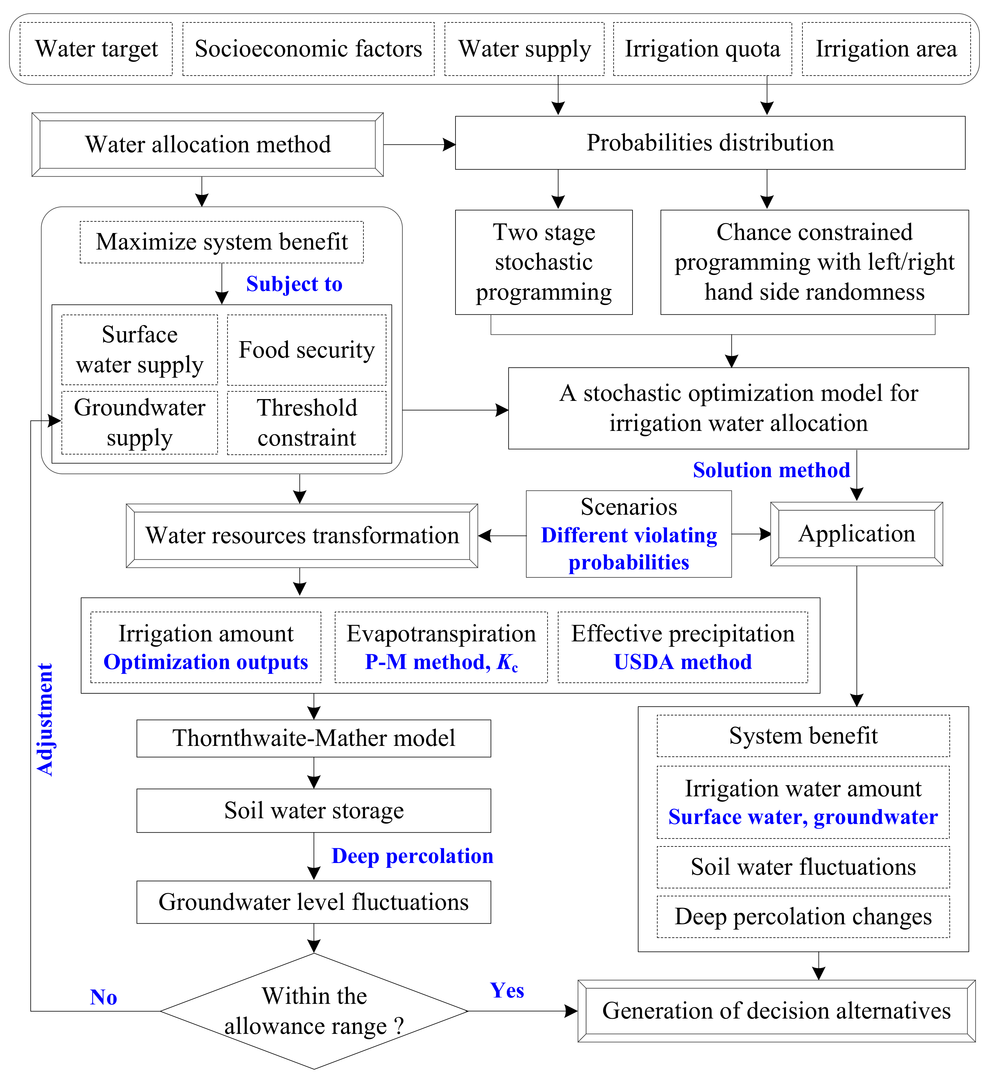
Considering a whole irrigation district as a system, the water allocation process assumes that every farmland in each time period provides its maximum (irrigation target) and minimum (fundamental water need to guarantee food security) water demand to determine agricultural irrigation water allocation strategies. The system could be irrigated with surface water, groundwater, or both together, and the optimization can therefore be conceptualized among different farmlands (different crops) during different time periods. For each farmland, the interaction among irrigation water (both surface water and groundwater), precipitation, and soil water is continuous with the changes of optimization outputs, which will directly affect the changes of groundwater level. In order to ensure that the groundwater level is within the allowance range when irrigating farmlands, integrating field water cycle processes with the optimization framework is necessary with groundwater supplies being considered as the adjustment variable. Considering the uncertainties because of nature factors and human activities, the randomness associated with the water supply and the irrigation quota is involved in order to minimize economic penalties due to any infeasibility, and provides decisions considering risk preferences with given probabilities. A detailed description of the decision-making framework is depicted in Figure 1.

2.2. Two-Stage Chance-Constrained Programming (TSCCP) with Left/Right-Hand-Side Randomness

2.2.1. Two-Stage Stochastic Programming

TSP with resources reflects a tradeoff between predefined strategies and the associated adaptive adjustments. In TSP, decision variables are divided into two categories: those that are determined before the random events occur, and those that (resource variables) are determined after the random events occur [15]. The TSP model can be expressed as follows [16]:

$$\max f={\displaystyle \sum _{j=1}^{J_1}{c}_j{x}_j}-{\displaystyle \sum _{j=1}^{J_2}{\displaystyle \sum _{l=1}^L{p}_l{d}_j{y}_{jl}}}$$

(1a)

Subject to:

$${\displaystyle \sum _{j=1}^{J_1}{a}_{ij}{x}_j\le b_i}\hspace{1em}\hspace{1em}\hspace{1em}\forall i=1,2,\cdots ,I$$

(1b)

$${\displaystyle \sum _{j=1}^{J_1}{a}_{ij}{x}_j+{\displaystyle \sum _{j=1}^{J_2}{a^{\prime }}_{kj}{y}_{jl}}}\ge {\tilde{\xi }}_l\hspace{1em}\hspace{1em}\hspace{1em}\forall k=1,2,\cdots ,K;\hspace{1em}l=1,2,\cdots ,L$$

(1c)

$$x_j\ge 0\hspace{1em}\hspace{1em}\hspace{1em}\forall j=1,2,\cdots ,J_1$$

(1d)

$$y_{jl}\ge 0\hspace{1em}\hspace{1em}\hspace{1em}\forall j=1,2,\cdots ,J_2;\hspace{1em}l=1,2,\cdots ,L$$

(1e)

where $x_j$ represents the first stage decision variables before the random variable is observed; $y_{jl}$ represents the second stage decision variables that are related to the resource actions against any infeasibilities arising due to particular realizations of the uncertainties; ${\tilde{\xi }}_l$ is the random variable with probability levels $p_l$ (${\displaystyle {\sum }_{l=1}^L{p}_l}=1$); $a_{ij}$, ${a^{\prime }}_{kj}$, $c_j$, $d_j$, and $b_i$ are parameters.

2.2.2. Chance-Constrained Programming

CCP is useful for dealing with random uncertainty and reflecting the information risk of violating constraints. A general CCP problem can be presented as follows [17]:

$$\max f={\displaystyle \sum _{j=1}^J{c}_j{x}_j}$$

(2a)

This is subject to:

$$\mathrm{Pr}\left\{{\displaystyle \sum _{j=1}^J{a}_{ij}{x}_j\le b_i\left(\omega \right)}\right\}\ge 1-q_i\hspace{1em}\hspace{1em}\hspace{1em}\forall i=1,2,\cdots ,I$$

(2b)

$$x_j\ge 0\hspace{1em}\hspace{1em}\hspace{1em}\forall j=1,2,\cdots ,J$$

(2c)

where $\mathrm{Pr}\{\cdot \}$ denotes the probability of a random event $\{\cdot \}$; $b_i\left(\omega \right)$ is the right-hand-side parameter of the constraints that are expressed as random variables with a certain probability distribution. $q_i\left(q_i\in \left[0,1\right]\right)$ is the given level of the probability of the constraint, i.e., violating the levels which represent the admissible risk of constraint violating. $I$ is the number of CCP constraints. The meanings of other symbols are the same as model (1).

In order to solve model (2), the constraint (2b) should be converted into the corresponding deterministic linear equivalents with a series of predefined constraints-violation levels $p_i$:

$$a_{ij}{x}_j\le b_i{\left(\omega \right)}^{\left(q_i\right)}\hspace{1em}\hspace{1em}\hspace{1em}\forall i=1,2,\cdots ,I$$

(3)

where $b_i{\left(\omega \right)}^{\left(q_i\right)}=F^{-1}\left(q_i\right)$, representing the cumulative distribution function of $b_i\left(\omega \right)\left\{i.e.F_i\left[b_i\left(\omega \right)\right]\right\}$.

However, in many cases, some parameters in the left-hand-side constraints present randomness, and the above method is not capable of handling such cases. Therefore, a left-hand-side CCP constraint is formulated as follows:

$$\mathrm{Pr}\left\{{\displaystyle \sum _{j=1}^J{a}_{ij}\left(\omega \right)x_j\le b_i}\right\}\ge 1-q_i\hspace{1em}\hspace{1em}\hspace{1em}\forall i=1,2,\cdots ,I$$

(4)

where $a_{ij}\left(\omega \right)$ is the left-hand-side parameters of the constraints, which can be expressed as random variables with normal distributions for simplicity. Let ${\mu }_{ij}$ be the mean value and ${\sigma }_{ij}$ be the standard variation of random variables $a_{ij}\left(\omega \right)$. Because $a_{ij}\left(\omega \right)\sim N\left({\mu }_{ij},{\sigma }_{ij}^2\right)$, the linear combinations of its elements also follow normal distribution. Thus, we have:

$$\left[{\displaystyle \sum _{j=1}^J{a}_{ij}\left(\omega \right)x_j}\right]\sim N\left[{\displaystyle \sum _{j=1}^J{\mu }_{ij}{x}_j},{\displaystyle \sum _{j=1}^J{\left({\sigma }_{ij}{x}_j\right)}^2}\right]$$

(5)

Then, by transforming $a_{ij}\left(\omega \right)$ into standard normal random variables, Formula (4) can be expressed as follows:

$$\mathrm{Pr}\left\{\frac{{\displaystyle \sum _{j=1}^J{a}_{ij}\left(\omega \right)x_j}-{\displaystyle \sum _{j=1}^J{\mu }_{ij}{x}_j}}{\sqrt{{\displaystyle \sum _{j=1}^J{\left({\sigma }_{ij}{x}_j\right)}^2}}}\le \frac{b_i-{\displaystyle \sum _{j=1}^J{\mu }_{ij}{x}_j}}{\sqrt{{\displaystyle \sum _{j=1}^J{\left({\sigma }_{ij}{x}_j\right)}^2}}}\right\}\ge 1-q_i\hspace{1em}\hspace{1em}\hspace{1em}\forall i=1,2,\cdots ,I$$

(6a)

$$\iff \Phi \left(\frac{b_i-{\displaystyle \sum _{j=1}^J{\mu }_{ij}{x}_j}}{\sqrt{{\displaystyle \sum _{j=1}^J{\left({\sigma }_{ij}{x}_j\right)}^2}}}\right)\ge 1-q_i\hspace{1em}\hspace{1em}\hspace{1em}\forall i=1,2,\cdots ,I$$

(6b)

$$\iff \frac{b_i-{\displaystyle \sum _{j=1}^J{\mu }_{ij}{x}_j}}{\sqrt{{\displaystyle \sum _{j=1}^J{\left({\sigma }_{ij}{x}_j\right)}^2}}}\ge {\Phi }^{-1}\left(1-q_i\right)\hspace{1em}\hspace{1em}\hspace{1em}\forall i=1,2,\cdots ,I$$

(6c)

$$\iff {\Phi }^{-1}\left(1-q_i\right)\sqrt{{\displaystyle \sum _{j=1}^J{\left({\sigma }_{ij}{x}_j\right)}^2}}+{\displaystyle \sum _{j=1}^J{\mu }_{ij}{x}_j}\le b_i\hspace{1em}\hspace{1em}\hspace{1em}\forall i=1,2,\cdots ,I$$

(6d)

${\Phi }^{-1}(\cdot )$ is the inverse function of the cumulative distribution function of a parameter that obeys the standardized normal distribution. Inequality (6d) enables the left-hand-side CCP to be dealt with by transforming the nonlinear programming into its approximated linearization form.

2.2.3. Model Structure of TSCCP with Left/Right-Hand-Side Randomness

The TSCCP with left/right hand-side randomness model can be formulated by integrating TSP and CCP with left and/or right-hand side randomness, and it can be expressed as follows:

$$\max f={\displaystyle \sum _{j=1}^{J_1}{c}_j{x}_j}-{\displaystyle \sum _{j=1}^{J_2}{\displaystyle \sum _{l=1}^L{p}_l{d}_j{y}_{jl}}}$$

(7a)

This is subject to:

$$\mathrm{Pr}\left\{{\displaystyle \sum _{j=1}^{J_1}{a}_{i_{1}j}{x}_j\le b_{i_1}\left(\omega \right)}\right\}\ge 1-q_{i_1}\iff a_{i_{1}j}{x}_j\le b_{i_1}{\left(\omega \right)}^{\left(q_i\right)}\hspace{1em}\hspace{1em}\hspace{1em}\forall i_1=1,2,\cdots ,I_1$$

(7b)

$$\mathrm{Pr}\left\{{\displaystyle \sum _{j=1}^{J_1}{a}_{i_{2}j}\left(\omega \right)x_j\le b_{i_2}}\right\}\ge 1-q_{i_2}\iff {\Phi }^{-1}\left(1-q_{i_2}\right)\sqrt{{\displaystyle \sum _{j=1}^J{\left({\sigma }_{i_{2}j}{x}_j\right)}^2}}+{\displaystyle \sum _{j=1}^J{\mu }_{i_{2}j}{x}_j}\le b_{i_2}\hspace{1em}\hspace{1em}\hspace{1em}\forall i_2=1,2,\cdots ,I_2$$

(7c)

$${\displaystyle \sum _{t=1}^T{m}_{tj}{x}_j}\le n_t\hspace{1em}\hspace{1em}\hspace{1em}\forall t=1,2,\cdots ,T$$

(7d)

$${\displaystyle \sum _{j=1}^{J_1}{a}_{ij}{x}_j+{\displaystyle \sum _{j=1}^{J_2}{a^{\prime }}_{kj}{y}_{jl}}}\ge {\tilde{\xi }}_l\hspace{1em}\hspace{1em}\hspace{1em}\forall k=1,2,\cdots ,K;\hspace{1em}l=1,2,\cdots ,L$$

(7e)

$$x_j\ge 0\hspace{1em}\hspace{1em}\hspace{1em}\forall j=1,2,\cdots ,J_1$$

(7f)

$$y_{jl}\ge 0\hspace{1em}\hspace{1em}\hspace{1em}\forall j=1,2,\cdots ,J_2;\hspace{1em}l=1,2,\cdots ,L$$

(7g)

where $m_{tj}$ and $n_j$ are parameters.

2.3. TSCCP for Irrigation Allocation Considering Water Resources Transformation

2.3.1. Optimization Model for Irrigation Water Allocation

The aim of the optimization model for irrigation water allocation is to allocate limited surface water and groundwater resources to different farmlands corresponding to different crops in an irrigation district during each time period. The model structure is the TSCCP with left/right-hand-side randomness. The objective function is the maximization of system economic benefits, considering the variations of different flow levels, and it can be expressed as follows:

$$\max F=\max \left\{{\displaystyle \sum _{c=1}^C{\displaystyle \sum _{s=1}^S{\displaystyle \sum _{t=1}^{T}B{C}_c}\cdot W{P}_c\cdot W{T}_{cst}-{\displaystyle \sum _{c=1}^C{\displaystyle \sum _{s=1}^S{\displaystyle \sum _{t=1}^T{\displaystyle \sum _{l=1}^L{p}_l}\cdot P{C}_{cst}\cdot W{S}_{cstl}}}}}}\right\}$$

(8a)

where $c$ denotes the crop types and the total number of crops is $C$, $s$ denotes the water sources and the total number of water sources is $S$, $t$ denotes the time period and the total number of time periods during the whole growth period of crops is $T$, $l$ denotes the flow level and its total number is $L$; $B{C}_c$ is the benefit coefficient of crop $c$, in RMB/kg (RMB is the Chinese currency unit); $W{P}_c$ is the water productivity of crop $c$, in kg/m³, $W{T}_{cst}$ is the water target of crop $c$ with water source $s$ in time period $t$ in m³, $p_l$ is the occurrence probability of flow level $l$, $P{C}_{cst}$ is the penalty coefficient of crop $c$ with water source $s$ in time period $t$ in RMB/m³, and $W{S}_{cstl}$ (decision variable) is the water shortage of crop $c$ with water source $s$ in time period $t$ under flow level $l$ in m³. $W{T}_{cst}-W{S}_{cstl}$ indicates the water allocation amount to crop $c$ with water source $s$ in time period $t$ under flow level $l$ in m³.

The objective function subjects to the following constraints:

(1) Surface water supply constraint

The surface water allocation in each time period under each flow level should not be larger than surface water supply. As the water supply greatly depends on the runoff with a randomness characteristic, this constraint is expressed as CCP with right-hand-side randomness, and it can be described as follows:

$$\mathrm{Pr}\left\{\omega |{\displaystyle \sum _{c=1}^C\left[W{T}_{c\left(s=1\right)t}-W{S}_{c\left(s=1\right)tl}\right]}/\left({\eta }_c\cdot {\eta }_f\right)\le SWS{\left(\omega \right)}_{tl}\right\}\ge 1-q_{SWS}\hspace{1em}\hspace{1em}\hspace{1em}\forall t,l$$

(8b)

where, ${\eta }_c$ is the water use efficiency coefficient of canal water and is dimensionless, ${\eta }_f$ is the water use efficiency coefficient of the field and is dimensionless, $SWS{\left(\omega \right)}_{tl}$ is the surface water supply in time period $t$ under flow level $l$ in m³, and $q_{SWS}$ is the violating probability of the surface water supply constraint.

(2) Groundwater supply constraint

Similarly to surface water supply constraint, the groundwater allocation in each time period should not be larger than the groundwater supply. The fluctuation of groundwater is much smaller than the surface water and the changes of groundwater under different flow levels are insignificant. Therefore, this constraint is not expressed as CCP. However, it is worth noting that the groundwater supply can potentially be adjusted based on the results of the water resource transformation process in order to guarantee the rational exploitation of groundwater. This constraint can be expressed as follows:

$${\displaystyle \sum _{c=1}^C\left[W{T}_{c\left(s=2\right)t}-W{S}_{c\left(s=2\right)tl}\right]}/{\eta }_f\le GW{S}_t\hspace{1em}\hspace{1em}\hspace{1em}\forall t,l$$

(8c)

where $GW{S}_t$ is the groundwater supply in time period $t$ in m³.

(3) Food security constraint

The food demand for each crop should be satisfied to ensure people’s elementary needs. Food demand is related to population, irrigation quota, yield per unit area, and food demand standard. Among them, irrigation quota is greatly affected by hydro-meteorological conditions and human elements, which lead to the randomness of the irrigation quota. Therefore, this constraint is expressed as CCP with left-hand-side randomness, and it can be described as follows:

$$\mathrm{Pr}\left\{\omega |{\displaystyle \sum _{t=1}^T{\displaystyle \sum _{s=1}^S\left[Y{A}_c/IQ{\left(\omega \right)}_c\right]\cdot }\left(W{T}_{cst}-W{S}_{cstl}\right)\ge PO\cdot F{D}_c}\right\}\ge 1-q_{FS}\hspace{1em}\hspace{1em}\hspace{1em}\forall c,l$$

(8d)

where $Y{A}_c$ is the yield per unit area for crop $c$ in kg/ha, $IQ{\left(\omega \right)}_c$ is the irrigation quota of crop $c$ in m³/ha, $PO$ is the population of the whole irrigation district, $F{D}_c$ is the food demand of crop $c$ in kg/capita, and $q_{SWS}$ is the violating probability of the food security constraint.

(4) Maximum irrigation constraint

In order to avoid water waste, water allocation, including both surface water and groundwater to each crop under each flow level, should not be larger than the maximum irrigation amount during the whole crop growth period. This constraint can be expressed as follows:

$${\displaystyle \sum _{s=1}^S{\displaystyle \sum _{t=1}^T\left(W{T}_{cst}-W{S}_{cstl}\right)}}\le IW{A}_{\max ,c}\hspace{1em}\hspace{1em}\hspace{1em}\forall c,l$$

(8e)

where $IW{A}_{\max ,c}$ is the maximum irrigation water amount for crop $c$ in m³.

(5) Water allocation constraint

Water allocation amount to each crop with each water source in each time period under each flow level should be non-negative. This constraint can be expressed as follows:

$$W{T}_{cst}-W{S}_{cstl}\ge 0\hspace{1em}\hspace{1em}\hspace{1em}\forall c,s,t,l$$

(8f)

(6) Non-negative constraint

The decision variables of the model should be non-negative. This constraint can be expressed as follows:

$$W{S}_{cstl}\ge 0\hspace{1em}\hspace{1em}\hspace{1em}\forall c,s,t,l$$

(8g)

2.3.2. Field Water Cycle Process

The transformation among surface water, precipitation, soil water, and groundwater is considered when optimizing agricultural irrigation water. The revised Thornthwaite–Mather (T–M) model which was developed by Thornthwaite and Mather [18], with a detailed study of the model done by Alley [19], is used to calculate the changes of soil water storage and deep percolation [20], and this will help to amend the irrigation water allocation results. There exists a basic assumption when using the T–M model, i.e., the evapotranspiration rate decreases linearly from a maximum value, when the soil water content corresponds to field capacity, to zero, when the soil reaches the permanent wilting point. The time step of the T–M model is usually in months. The fluctuations of the soil moisture in the unsaturated zone depend on whether the water supply including precipitation and irrigation water (results of the optimization model) of month $t$, i.e., $EP\left(t\right)+I\left(t\right)$, is greater or less than the reference evapotranspiration for the month $PET\left(t\right)$. The $PET\left(t\right)$ in a certain time period can be calculated by the PM-ET₀ method [21] and the effective precipitation $EP\left(t\right)$ can be estimated using the empirical formulae derived from the USDA Soil Conservation Service [22].

When $EP\left(t\right)+I\left(t\right)\le PET\left(t\right)$, the soil moisture content can be described as:

$$S\left(t\right)=S\left(t-1\right)\exp \left\{-\left[PET\left(t\right)-EP\left(t\right)-I\left(t\right)\right]/\left(S_{fc}-S_{wp}\right)\right\}$$

(9)

where $S_t$, $S_{t-1}$ represent soil moisture content in the root zone at the beginning and the end of the time period, respectively, in mm; $S_{fc}$ and $S_{wp}$ denote soil water content in the point of field capacity and permanent wilting point, respectively; $S_{fc}-S_{wp}$ represents the water holding capacity in the root zone. In the above case, the deep percolation ($\Delta DP\left(t\right)$) equals 0.

When $EP\left(t\right)+I\left(t\right)\ge PET\left(t\right)$, the soil moisture content is updated by:

$$S\left(t\right)=\min \left[EP\left(t\right)+I\left(t\right)-PET\left(t\right)+S\left(t-1\right),\left(S_{fc}-S_{wp}\right)\right]$$

(10)

The excess precipitation and irrigation water are assumed to contribute to deep percolation. In such a case, the deep percolation can be expressed as:

$$\Delta DP\left(t\right)=\left[EP\left(t\right)+I\left(t\right)-PET\left(t\right)+S\left(t-1\right)-\left(S_{fc}-S_{wp}\right)\right]$$

(11)

2.3.3. Solution Method

The steps for solving the optimization model for irrigation water allocation based on the TSCCP with left/right-hand-side randomness considering the field water resources transformation process, are described as follows:

Step 1: Formulate the TSCCP model with left/right-hand-side randomness for irrigation water allocation (i.e., model (8)).

Step 2: Linearize the CCP constraints under the given violating probabilities. Specifically, for the CCP with right-hand-side randomness, the theoretical distribution curve should be fitted first, based on which, the values corresponding to each given violating probability can be determined. For the CCP with left-hand-side randomness, the normal probability distribution was assumed. Then, the CCP can be transformed into the corresponding linear form according to (6d) based on the mean value and the standard deviation value of the samples.

Step 3: Give an initial value of groundwater supply, and solve the optimization model by coding in an optimization software and recording the outputs.

Step 4: Input the outputs of the optimization into the T-M model to estimate the soil moisture and deep percolation.

Step 5: Judge whether the changes of groundwater levels in each time period can be calculated based on whether the deep percolation and irrigation area is within the range of permissible fluctuations (i.e., the range between groundwater levels that can cause overexploitation and soil salinization). If yes, output the results, if no, adjust the value of groundwater supply, and repeat steps 3 and 4.

Step 6: Give different violating probabilities corresponding to different kinds of CCP, and solve the framework by repeating steps from 2 to 5 to analyze the sensitivity of the model.

3. Case Study

3.1. Description of the Study Area

The Yingke irrigation district (38°50′–38°58′ N, 100°17′–100°34′ E), located in the middle reaches of Heihe River basin, Northwest China, was chosen as the study area to test the developed model. The Yingke irrigation district is the third largest irrigation district in the middle reaches, and it belongs to a semi-arid area with a water shortage problem. The climate is typically a cold, arid continental climate with an annual average precipitation and a reference evapotranspiration of around 125 mm and 1200 mm, respectively. More than 90% of the water supply for Yingke irrigation district is used for irrigating crops. The other 10% of the water supply is used for forestry and grass irrigation, and human and livestock drinking. The major crops are corn, including grain corn and forage corn, and spring wheat, with their cropped areas accounting for 83% of the total crop area. Commercial crops such as vegetables and melons take up a 15% proportion of the area [23]. The irrigation season is usually from April to September. Because of water shortage, groundwater is also exploited as supplemental water supply source. However, the poor irrigation management has led to an imbalanced distribution of various crops in different time periods, and a lower irrigation efficiency. This leads to the necessity for exploring optimal irrigation corresponding to different flow levels, considering field water resources transformation processes and allocation uncertainties to improve the present water use situations and economic benefits.

3.2. Data Collection

There are two pieces of data: data for the optimization model, and data for the T-M model. For the optimization model, water supply, water target, irrigation quota, and socioeconomic factors including benefit coefficient, penalty coefficient, population, food demand standard, irrigation area, and maximum irrigation amount, and engineering elements such as water use efficiency for canal and field.

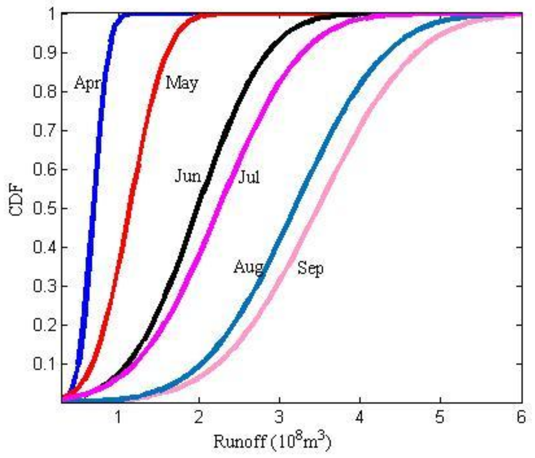
Surface water supply for Yingke irrigation district is taken from Heihe river. In this study, it was assumed that the monthly variation of surface water supply for Yingke irrigation district was consistent with that of the runoff of Heihe River at Yingluoxia hydrometric station (the boundary point of the upper and the middle reaches of Heihe River basin). Therefore, if runoff from Yingluoxia hydrometric station was known, the surface water supply for Yingke irrigation district could be obtained, and it was expressed a random variable. The ${\chi }^2$ hypothesis testing shows that the monthly runoff of Yingluo hydrometric station obeys normal distribution at a 0.1 significance level. Therefore, the normal distribution can be used to solve the CCP problems. Three flow levels were applied, and the category of different flow levels was based on the frequency analysis method. Let P express the frequency for dividing different flow levels, then $P\le 25\%$ corresponds to a high flow level, $25\%<P\le 75\%$ corresponds to a middle flow level and $P>75\%$ corresponds to a low flow level. The mathematical expectation method was used to calculate P [24]. The runoff data of Yingluoxia was ranked in descending order, and the ranked series was recorded as $\left\{x_1,x_2,\cdots ,x_m,\cdots ,x_n\right\}$. Then P can be expressed as $P=\left(m/\left(n+1\right)\times 100\%\right)$, with m denoting the number of “greater than” and “equal to” $x_m$, and n denoting the total number of historical data. Using this formula, different flow levels can be divided, based on the division categories of P. Then, the occurrence probabilities of each flow level could be obtained by dividing the number of years of each flow level by the total number of years (from 1944 to 2014). The occurrence probabilities for the high, middle, and low flow levels were 0.25, 0.5, and 0.25, respectively. The annual surface water supply for Yingke irrigation district accounted for approximately 8.7% of the runoff from Yingluoxia hydrometric station. Then, the water supply during the whole crop growth period (From April to September) could be obtained. Based on the proportionality coefficient, the monthly water supply of the Yingke irrigation district could be obtained. The proportionality coefficients were 0.05, 0.09, 0.16, 0.27, 0.25, and 0.18 for April, May, June, July, August, and September, respectively. The water supply for Yingke irrigation district can be seen in

Table 1. Water supply.

Month	Surface Water Supply (104 m3)			Groundwater Supply (104 m3)
	High Flow Level	Middle Flow Level	Low Flow Level
April	1002.45	751.20	585.90	961.87
May	1813.80	1242.94	822.54	1001.84
June	3260.92	2169.82	1367.87	1031.62
July	5265.86	3796.17	2672.32	1049.64
August	5080.22	3482.88	2516.90	1005.45
September	3902.22	2456.99	1618.69	949.58

. Based on the monthly observation data of runoff from Yingluoxia hydrometric station, the cumulative probability distributions of each month from April to September (the main irrigation period) were fitted, as shown in Figure 2. Based on the figure, the surface water supply under the selected violating probabilities was obtained. In this study, the violating probabilities were selected as 0.01, 0.05, 0.1, 0.15, and 0.2. The initial groundwater supply was from Annual Water Conservation Report of Zhangye City (AWC Report for short thereafter) from 2010 to 2016, and it was listed in Table 1. The proportions of agricultural irrigation water supply under high, middle, and low flow levels were 0.94, 0.92, and 0.9, respectively. The soil type of the Yingke irrigation district was silt loam and loam. According to the study of Li et al. (2015) [25], the permissible critical groundwater depth of 2 m was set to avoid salinization. If the groundwater depth is less than 2 m, the optimal water allocation results should be amended by re-calculating the optimization model with an adjustment of groundwater supply. The changes of groundwater depth for each time period can be obtained from the ratio of deep percolation amount and the irrigation area, and the deep percolation amount can be obtained by the Formula (11).

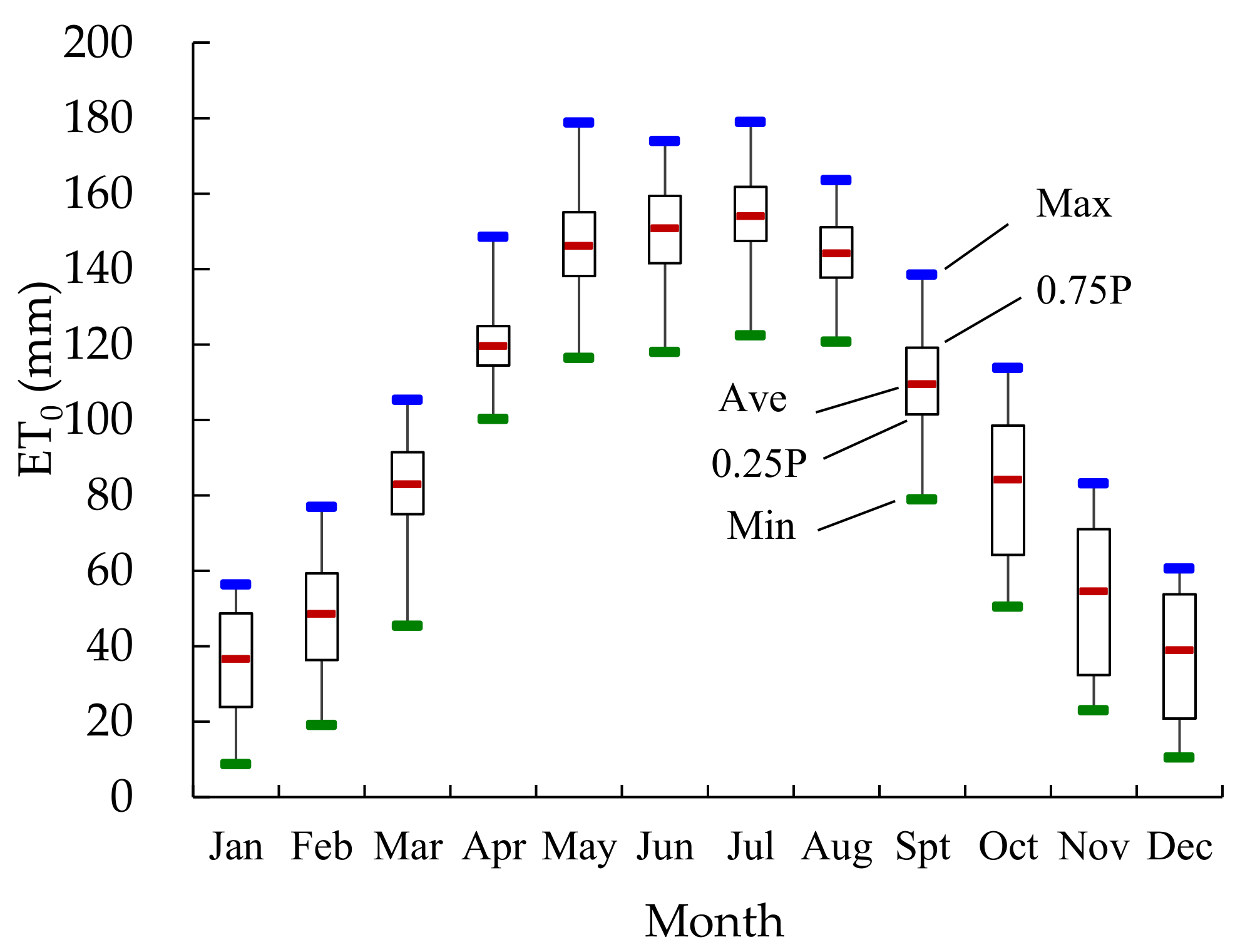
Water target per unit area in this study was considered as crop demand and it was the numerical equivalent of crop evapotranspiration, which was estimated by multiplying the crop coefficient (K_c) with the reference evapotranspiration (ET₀). ET₀ was calculated by the PM-ET₀ method on the basis of meteorological data from 1956 to 2014, and the monthly changes of ET₀ is shown in Figure 3. The values of K_c and the calculated ET₀ were listed in

Table 2. K_c and ET₀.

Month	ET0	Kc
	(mm)	Grain Corn	Forage Corn	Wheat	Vegetables
April	119.61	0.22	0.20	0.30	0.44
May	146.23	0.50	0.44	1.15	0.8
June	150.85	1.16	0.53	1.15	1
July	154.11	1.20	1.46	0.93	0.99
August	144.20	1.20	1.14	-	0.565
September	109.52	0.60	1.22	-	0.55

. The water targets corresponding to different water sources were obtained by the proportionality coefficients of the surface water supply and the groundwater supply. The proportionality coefficients were obtained based on long-term statistical information. For surface water (groundwater), the proportionality coefficients were 0.44 (0.56), 0.55 (0.45), 0.68 (0.32), 0.78 (0.22), 0.78 (0.22), and 0.72 (0.28) for April, May, June, July, August, and September, respectively. Then the irrigation area was used to transform the water target per unit area into the volume. In this study, the climate change effects were considered. According to previous studies [26], when the temperature increased by 1 °C, 2 °C, 3 °C, and 4 °C, water demand for crops increased 1.03–1.04-fold, 1.06–1.07-fold, 1.09–1.10-fold, and 1.13–1.14-fold over the current situation, respectively. Therefore, the calculated water target was re-defined considering this rise. A temperature rise of 2 °C was considered, based on the study of Wang and Chen (2014) [27]. The water target was listed in

Table 3. Water targets.

Crops	Water Sources	Water Target (104 m3)
		April	May	June	July	August	September
Grain corn	Surface water	79.60	276.96	804.14	974.94	904.11	320.34
	Groundwater	94.80	207.62	355.57	250.71	242.74	115.15
Forage corn	Surface water	53.43	179.96	271.29	875.87	634.21	480.96
	Groundwater	63.63	134.91	119.96	225.24	170.28	172.88
Wheat	Surface water	14.98	87.92	110.03	104.29	0.00	0.00
	Groundwater	17.84	65.91	48.65	26.82	0.00	0.00
Vegetables	Surface water	55.98	155.82	243.76	282.83	149.69	103.26
	Groundwater	66.67	116.81	107.79	72.73	40.19	37.12

.

In this study, irrigation quota was a random variable on the left-hand side of the CCP constraint, and it was assumed to obey a normal distribution. Based on the statistical data from the AWC Report from 2000 to 2015, the mean value and the standard deviation of each crop were calculated (see

Table 4. Parameters for crops.

Parameter	Unit	Grain Corn	Forage Corn	Wheat	Vegetables
Irrigation quota (mean)	m3/ha	4534.33	5001.09	5240.02	7604.99
Irrigation quota (standard deviation)	m3/ha	382.23	421.57	308.65	447.95
Benefit coefficient	RMB/kg	3.00	2.31	2.28	3.45
Water productivity	kg/m3	1.84	1.67	1.63	7.99
Planting area	ha	6025.00	4448.82	831.57	2118.60
Yield per unit area	kg/ha	8343.30	8340.30	8554.65	60746.7
Maximum irrigation amount	104m3	4397.29	3718.66	462.90	1302.40

). The violating probabilities of 0.01, 0.05, 0.1, 0.15, and 0.2 were also applied to the irrigation quota when transforming the CCP with left-hand-side randomness into the corresponding linear form. The values of some socioeconomic parameters in the optimization model varied with different crops, and they are listed in Table 4. The penalty coefficient was related to the degree of the water demand besides the crop types (see

Table 5. Penalty coefficient.

Crops	Penalty Coefficient (RMB/m3)
	April	May	June	July	August	September
Grain corn	6.07	6.68	7.89	8.50	8.50	7.29
Forage corn	4.05	4.46	4.86	6.08	5.27	5.67
Wheat	3.90	4.68	4.68	4.29	-	-
Vegetables	31.69	41.20	47.54	44.37	38.03	34.86

). The acquisition of these parameters was based on the AWC report, the year book of Zhangye City, field investigations, and relative references. Among them, the maximum irrigation amount was obtained by calculating the extremum of the quadratic water production function (WPF). The WPF for each crop was fitted by [2]. The population of the Yingke irrigation district was 16.44 × 10⁴ people. The average water use efficiency for the canal was 0.68 based on data from 2000 to 2015 of the AWC report, and the average water use efficiency for the field referred to [23].

Data for the field water cycle process mainly included effective precipitation, reference evapotranspiration, and soil-relevant parameters. According to the empirical formulae derived from the USDA Soil Conservation Service, the effective precipitation for each month from April to September were calculated and they were 3.72 mm, 3.95 mm, 19.49 mm, 23.06 mm, 28.52 mm, and 19.9 mm respectively. The reference evapotranspiration was calculated by the PM-ET₀ method, and the results can be seen in Figure 3 and Table 2. The initial soil moisture content was set to 25%, the field capacity was 35% and the permanent wilting point was 10%. The root zone was set to 1 m with loamy soil. The average groundwater level depths for each month during the irrigation period were 3.25 m for April, 3.38 m for May, 3.48 m for June, 3.55 m for July, 3.40 m for August, and 3.21 m for September, according to observation data from 12 stations in the Yingke irrigation district.

4. Results and Discussion

4.1. Irrigation Water Allocation

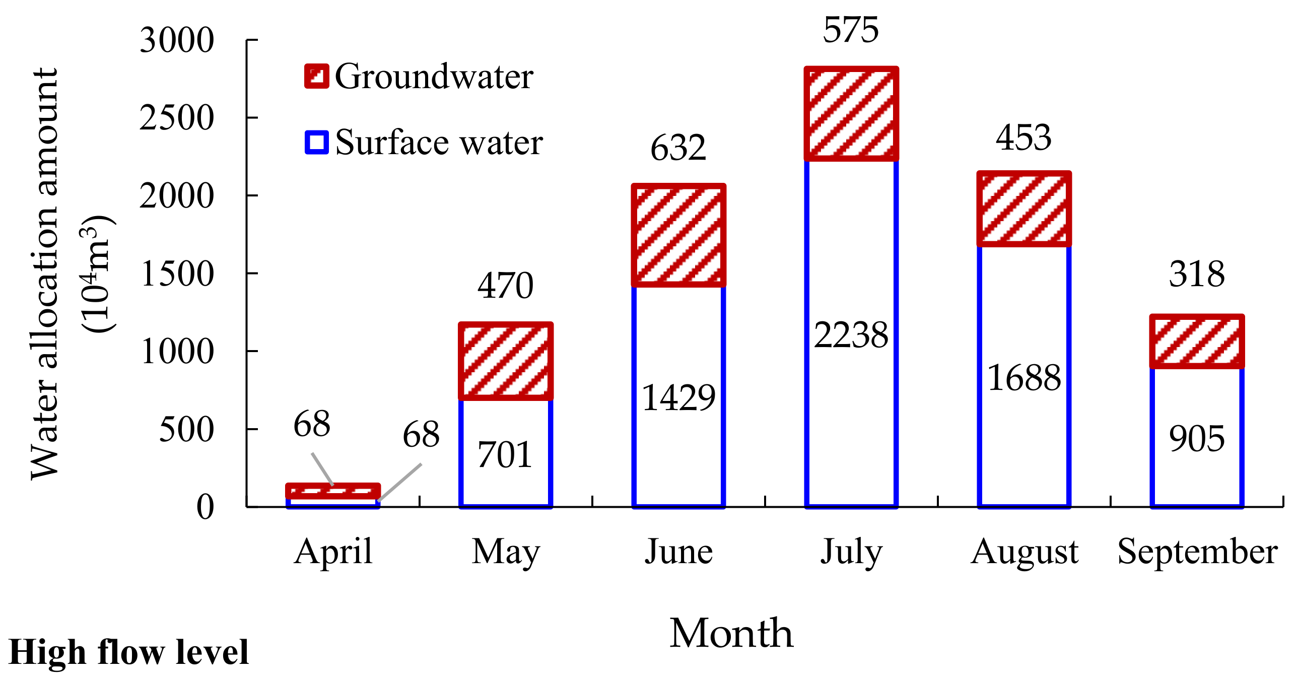
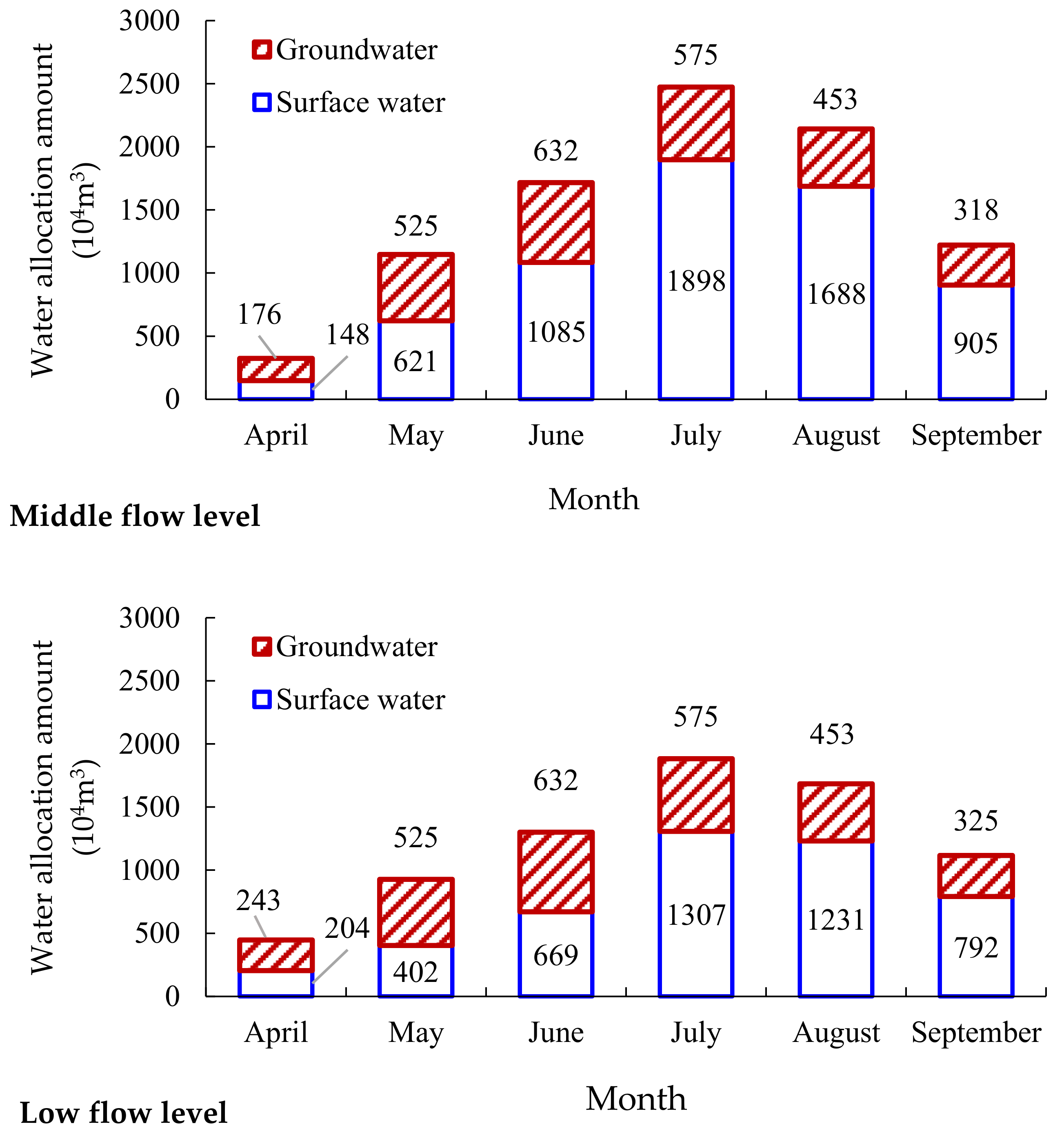
Irrigation water allocation results (both surface water and groundwater) for each crop in each time period under each flow level were obtained by solving the optimization model, considering the different terms of the water balance. The Irrigation water for all crops in the Yingke irrigation district is shown in Figure 4. It was obvious that water allocation amount under a high flow level (9545 × 10⁴ m³) was larger than under a middle flow level (9023 × 10⁴ m³), and the last one was under a low flow level (7359 × 10⁴ m³), attributing to the surface water supply. June, July, and August were the months in which the peaks of water demand were concentrated. Water allocation in this period was 74% (high flow level), 70% (middle flow level), and 66% (low flow level), for the whole irrigation period. Surface water allocations for the three flow levels were 7029 × 10⁴ m³ for the high flow level, 6344 × 10⁴ m³ for the middle flow level, and 4605 × 10⁴ m³ for the low flow level. In order to alleviate water resources shortage as well as improve system economic benefits in unfavorable cases (middle and low flow levels), groundwater allocation increased from a higher flow level to a lower flow level, i.e., 2516 × 10⁴ m³ for a high flow level, 2680 × 10⁴ m³ for a middle flow level, and 2754 × 10⁴ m³ for a low flow level. It indicated that groundwater could be regarded as a regulative water source at a reasonable range to improve irrigation water allocation patterns in the Yingke irrigation district.

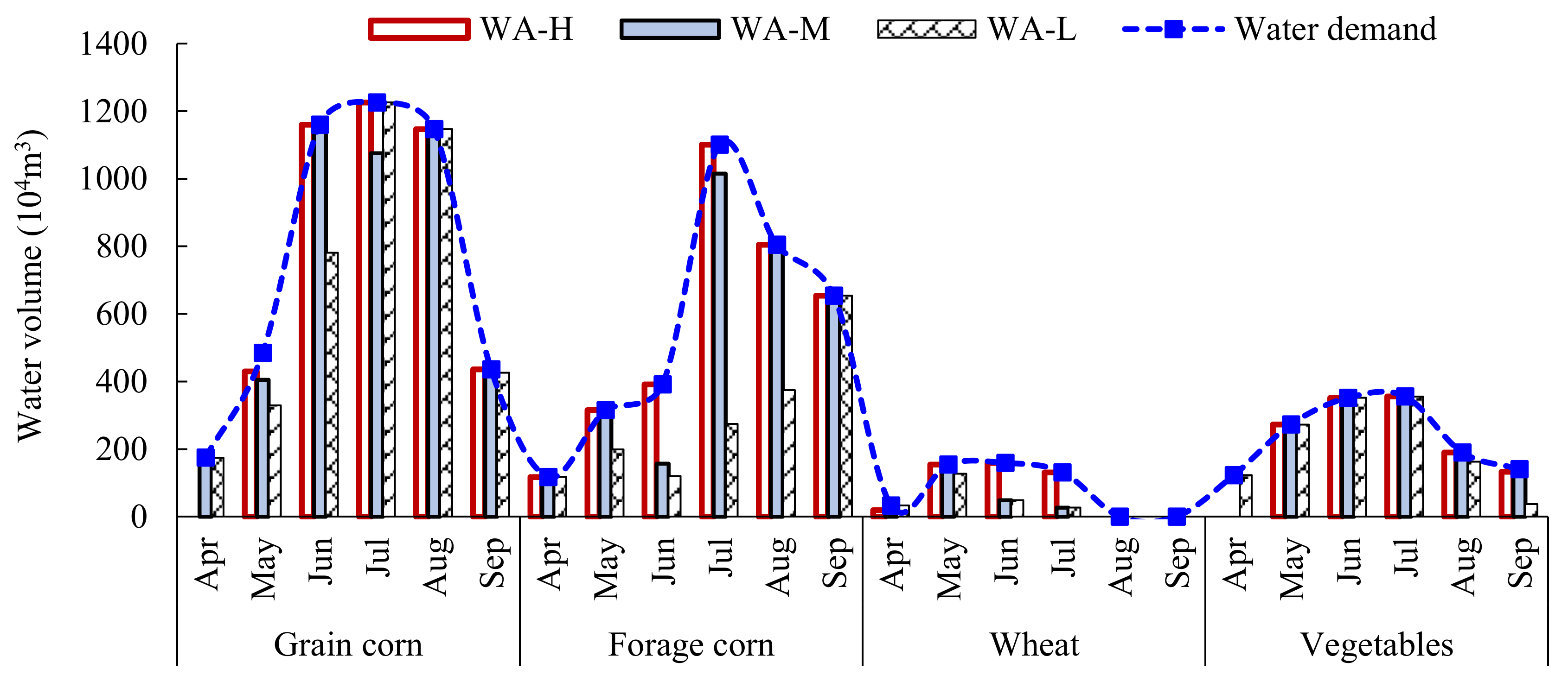
Figure 5 shows the total irrigation water allocation amount (the sum of surface water and groundwater irrigation amounts) for each crop in each month under the three flow levels. Corn, including grain corn and forage corn, occupied 80% of the total irrigation water allocation amount, reflecting the superiority in planting corn in the Yingke irrigation district. Corn was the major food crop in Yingke irrigation district, and the demand for corn was 376 kg per capita per year, with grain corn accounting for 53%, and forage corn accounting for 47%. The demand for wheat was only 23.3 kg per capita per year for its lower benefit and higher water consumption. It can be seen from the figure that the water demand for the vegetables was given precedence for its higher economic benefit and higher penalty coefficient. In other words, if the water shortage for vegetables was larger, then the system benefit would be decreased as the current optimal results. From the figure, water allocation law for grain corn and forage corn was different. For grain corn, water allocation from June to August was the irrigation peak, while for forage corn, water allocation from July to September was the irrigation peak. This was because of the crop coefficient K_c (see Table 2), which directly affected the water demand. The results indicated that the water allocation amount was sensitive to K_c, leading to the necessity of amending the parameter regularly for a specific area when optimizing irrigation water allocation.

4.2. System Benefit under Different Scenarios

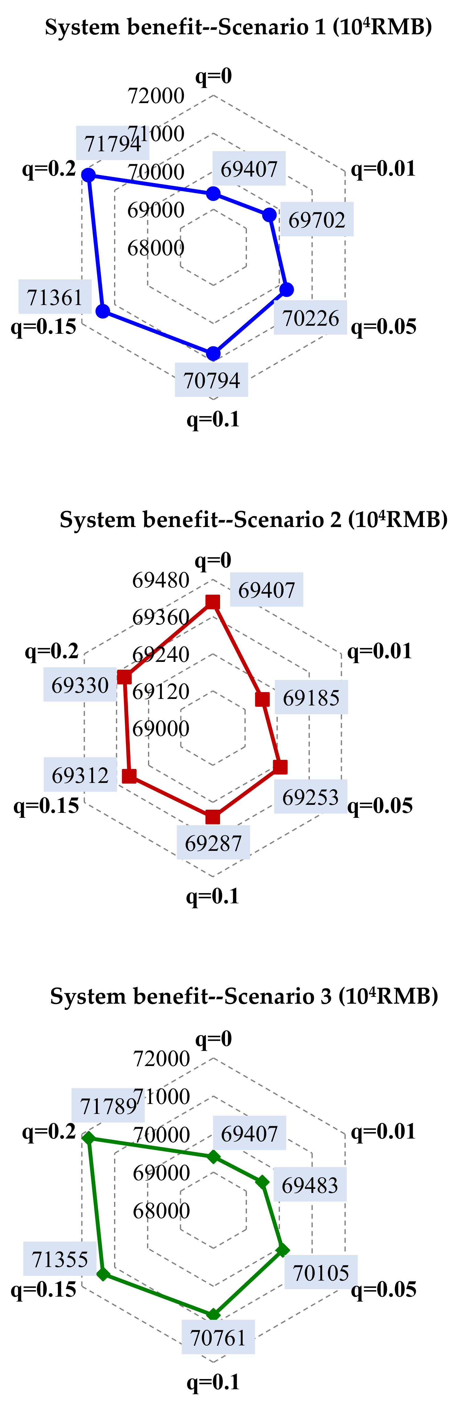
The above results were obtained without considering the CCP constraints. However, two types of CCP constraints (Equations (8b) and (8d)) were incorporated into the optimization model, and the violating probabilities for each CCP constraint were 0.01, 0.05, 0.1, 0.15, and 0.2. Therefore, three scenarios were generated: Scenario 1, where the violating probabilities of the surface water supply constraint (surface water supply was the random variable in the right-hand side of the CCP constraint) were changed from 0.01 to 0.2, while the violating probability of the food security constraint (irrigation quota was the random variable in the left-hand side of the CCP constraint) was fixed at 0; Scenario 2, where the violating probabilities of the food security constraint were changed from 0.01 to 0.2, while the violating probability of the water supply constraint was fixed at 0; Scenario 3, where the violating probabilities of both the two constraints were changed from 0.01 to 0.2 simultaneously. Different violating probabilities affected the decision strategies for irrigation, and thus affected the system economic benefit, as illustrated in Figure 6. In Scenario 1, the system benefit increased as the violating probabilities increased. This was because a larger violating probability indicated a larger water supply that would contribute to a higher system benefit, because the objective function was linear. However, due to the uncertainty associated with the probability of occurrence of a certain water supply, a risk would be generated. Larger probabilities meant larger risks. Therefore, whether the violating probabilities should be considered and which one could be selected were largely dependent on the preference of the decision makers. In Scenario 2, the system benefit decreased as the violating probabilities increased, but the reduction was not dramatic. This was related to the property of the CCP constraints. Scenario 2 focused on the CCP with the left-hand-side randomness, i.e., the irrigation quota. According to the transformation method for solving such a kind of CCP, the inverse function of the cumulative distribution function of a parameter that obeys the standardized normal distribution should be calculated first. Larger violating probabilities corresponded to lower inverse function values. As the reciprocal of irrigation quota was used in the left-hand-side of food security constraint, larger violating probabilities led to larger reciprocal values, resulting in a lower water allocation amount in the case of the fixed right-hand-side values. Hence, the system benefit values under different violation probabilities showed a decreased trend. Because there was little changes of the annual variation of irrigation quota, the decline range of the system benefit was slight. Scenario 3 was the combined effect of Scenario 1 and Scenario 2, and it was obvious that the changing trend of system benefit in Scenario 3 was the same as Scenario 1 with different change extents. Compared with the two constraints, the results indicated that the optimization model was sensitive to surface water supply. Therefore, broadening water sources might be more efficient than reducing the water use in terms of decreasing irrigation quota to improve system benefits.

4.3. Soil Moisture and Deep Percolation

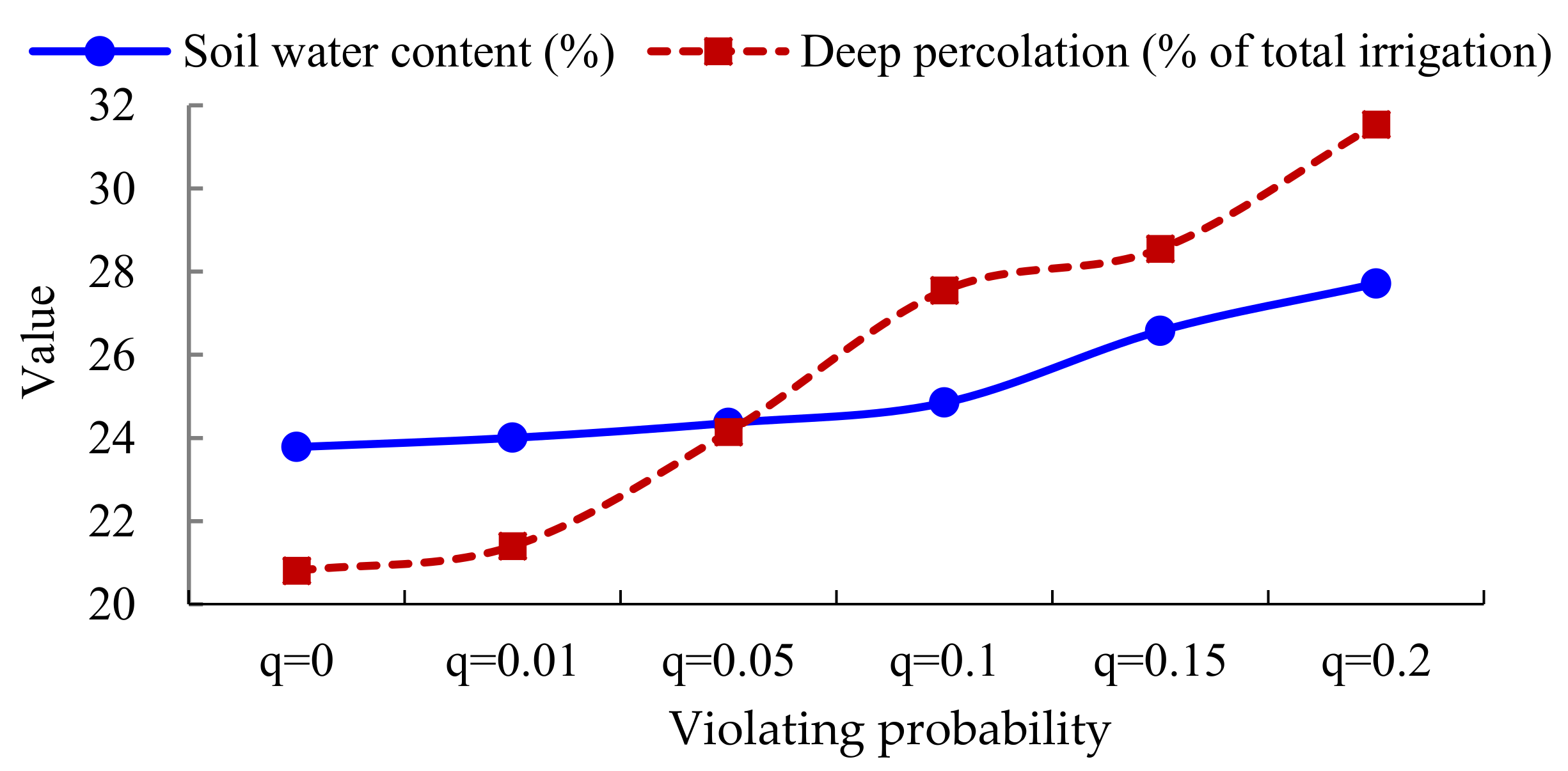
The field water cycle process was considered for adjusting the irrigation water allocation results. The outputs of the optimization model were input into the T-M model, and the average soil moisture and deep percolation were obtained, with the changes of groundwater level being considered as the correction condition. Taking Scenario 3 as an example, which could represent the combined effect of Scenario 1 and Scenario 2, the changes of soil water content and the ratio of deep percolation to the total irrigation amount was shown in Figure 7. It can be seen that soil moisture content presented an increase trend with an increase in violating probabilities. The reason was that larger violating probability corresponded to a larger irrigation water amount, and then this would lead to a larger soil moisture content until the value of the soil moisture content achieved the maximum soil moisture holding capacity, i.e., equal to the difference of soil water content between the field capacity and the permanent wilting point. If the soil moisture content exceeded the holding capacity, the deep percolation would be generated. For this study, the soil water content ranged from 23.78% to 27.71%, and the deep percolation rate ranged from 20.81% to 31.54%, with an increase in the violating probabilities. It should be noted that although a larger irrigation water amount would result in a higher system benefit based on the above results analysis, the irrigation water allocation amount would be restricted by two aspects, even if the water supply was sufficient. One restriction was the maximum irrigation amount, which was the upper threshold of the optimization model. If water allocation to a certain crop exceeded this threshold, a waste of water would be generated. This was attributed to the quadratic WPF (a convex quadratic function) for the whole growth period. The maximum irrigation amount corresponded to the maximum yield; in other words, if water continued to be allocated when the amount exceeded this value, the yield was expected to shrink, and the consequent system benefit would decrease. Another restriction was the groundwater level. Larger irrigation water amounts caused greater deep percolation. As the groundwater level depth in the Yinke district was fairly shallow, larger irrigation amounts might cause the groundwater level to rise, then give rise to soil salinization. This would affect crop growth, which is disadvantageous for improving the system economic benefit. Therefore, considering the field water resources transformation process was significant for adjusting the optimal irrigation water patterns.

4.4. Discussion

The aim of this paper is to develop a stochastic optimization method for irrigation water allocation, in which the field water cycle process (including the transformation of crop evapotranspiration, precipitation, irrigation, soil water content, deep percolation) was considered. By integrating a water balance model, the developed stochastic optimization method is capable of obtaining more accurate water allocation plans because the connection between surface water irrigation and groundwater irrigation was reflected, rather than dealing with the surface water and groundwater supplies as two individual components. In fact, there are several hydrological models that are able to describe field water cycle processes, such as the T-M model, the Belgium model, the Xin’anjiang model, the Guo model, the WatBal model, and the Schaake model. Each model has its own characteristics. However, this paper only took the T-M model as an example to examine the feasibility of integrating the field water balance model into the stochastic optimization framework, without comparing and demonstrating which model is appropriate and how different models affect water allocation strategies. This may become a major limit of the developed method, and requires future study.

For water-deficient regions, water-saving methods such as regulated deficit irrigation (RDI) or partial root zone drying (PRZD) are popular for reducing crop water consumption, and thus increasing irrigation efficiency. Considering different water-saving methods in the developed method is interesting, and alternative irrigation water allocation schemes in time-space under different scenarios can be provided. These methods directly affect the irrigation quota for each crop and soil water content, which are the main components of the optimization model, and thus they change the allocation strategies. However, how the RDI and PRZD affect the irrigation quota and soil water content is worth discussing with regards to field trials, and this was not discussed in this paper.

5. Conclusions

A TSCCP model with left/right-hand-side randomness, considering water resources transformation, has been developed for irrigation water allocation. The model is advantageous in: (1) effectively allocating limited surface water and groundwater supplies with consideration for field water resource transformations among irrigation water, precipitation, soil water, and groundwater to avoid unreasonable allocation schemes, with obtaining the maximum system economic benefit as the final aim; (2) dealing with randomness both in the right-hand side and left-hand side of constraints, which will help to generate irrigation water allocation schemes under different levels of water supply and different levels of constraint-violation risks.

The approach was applied to a real case study in an irrigation district in Northwest China, to demonstrate its feasibility. The results of irrigation water allocation for different crops in different months during the crops’ whole growth period under different flow levels, considering different violating probabilities, were obtained. The results gained insight into the tradeoffs between system benefit and economic penalties, with soil moisture content and deep percolation under different scenarios changing in an appropriate range, which are informative for decision makers. The approach is applicable for any irrigation district with water shortage issues. Future work will focus on improving the agro-hydrological model to acquire more accurate data on the field water cycle (actual evapotranspiration, soil water content, and deep percolation), and thus improving the practicality and applicability of the model.

References

- Galán-Martín, Á.; Vaskan, P.; Antón, A.; Esteller, L.J.; Guillén-Gosálbez, G. Multi-objective optimization of rainfed and irrigated agricultural areas considering production and environmental criteria: A case study of wheat production in Spain. J. Clean. Prod. 2017, 140, 816–830. [Google Scholar] [CrossRef]
- Jiang, Y.; Xu, X.; Huang, Q.; Huo, Z.; Huang, G. Optimizing regional irrigation water use by integrating a two-level optimization model and an agro-hydrological model. Agric. Water Manag. 2016, 178, 76–88. [Google Scholar] [CrossRef]
- Singh, A. An overview of the optimization modelling applications. J. Hydrol. 2012, 466, 167–182. [Google Scholar] [CrossRef]
- Davijani, M.H.; Banihabib, M.E.; Anvar, A.N.; Hashemi, S.R. Optimization model for the allocation of water resources based on maximization of employment in the agriculture and industry sectors. J. Hydrol. 2016, 533, 430–438. [Google Scholar] [CrossRef]
- Nguyen, D.C.H.; Dandy, G.C.; Maier, H.R.; Ascoug, J.C. Improved ant colony optimization for optimal crop and irrigation water allocation by incorporating domain knowledge. J. Water. Resour. Plan. Manag. 2016, 142, 04016025. [Google Scholar] [CrossRef]
- Xu, Y.; Li, W.; Ding, X. A stochastic multi-objective chance-constrained programming model for water supply management in Xiaoqing River watershed. Water 2017, 9, 378. [Google Scholar] [CrossRef]
- Guo, P.; Chen, X.; Li, M.; Li, J. Fuzzy chance-constrained linear fractional programming approach for optimal water allocation. Stoch. Environ. Res. Risk Assess. 2014, 28, 1601–1612. [Google Scholar] [CrossRef]
- Zhang, C.; Li, M.; Guo, P. An interval multistage joint-probabilistic chance-constrained programming model with left-hand-side randomness for crop area planning under uncertainty. J. Clean. Prod. 2017, 167, 1276–1289. [Google Scholar] [CrossRef]
- Maqsood, I.; Huang, G.; Yeomans, J.S. An interval-parameter fuzzy two-stage stochastic program for water resources management under uncertainty. Eur. J. Oper. Res. 2005, 167, 208–225. [Google Scholar] [CrossRef]
- Moghaddam, K.S.; DePuy, G.W. Farm management optimization using chance constrained programming method. Comput. Electron. Agric. 2011, 77, 229–237. [Google Scholar] [CrossRef]
- Li, M.; Guo, P. A coupled random fuzzy two-stage programming model for crop area optimization—A case study of the middle Heihe River Basin, China. Agric. Water Manag. 2015, 155, 53–66. [Google Scholar] [CrossRef]
- Karamouz, M.; Kerachian, R.; Zahraie, B. Monthly water resources and irrigation planning: Case study of conjunctive use of surface and groundwater resources. J. Irrig. Drain. Eng. 2004, 130, 93–98. [Google Scholar] [CrossRef]
- Wu, X.; Zheng, Y.; Wu, B.; Tian, Y.; Han, F.; Zheng, C. Optimizing conjunctive use of surface water and groundwater for irrigation to address human-nature water conflicts: A surrogate modeling approach. Agric. Water Manag. 2016, 163, 380–392. [Google Scholar] [CrossRef]
- Li, X.; Huo, Z.; Xu, B. Optimal allocation method of irrigation water from river and lake by considering the field water cycle process. Water 2017, 9, 911. [Google Scholar] [CrossRef]
- Li, Y.; Huang, G. Two-stage planning for sustainable water-quality management under uncertainty. J. Environ. Manag. 2009, 90, 2402–2413. [Google Scholar] [CrossRef] [PubMed]
- Li, W.; Li, Y.; Li, C.; Huang, G. An inexact two-stage water management model for planning agricultural irrigation under uncertainty. Agric. Water Manag. 2010, 97, 1905–1914. [Google Scholar] [CrossRef]
- Charnes, A.; Cooper, W.W. Response to decision problems under risk and chance constrained programming: Dilemmas in the transitions. Manag. Sci. 1983, 29, 750–753. [Google Scholar] [CrossRef]
- Thornthwaite, C.W.; Mather, J.R. The Water Balance; Publications in Climatology; Laboratory of Climatology, Drexel Instatute of Technology: Centerton, NJ, USA, 1995; Volume 8, pp. 1–104. [Google Scholar]
- Alley, W.M. On the treatment of evapotranspiration, soil moisture accounting and aquifer recharge in monthly water balance models. Water Resour. Res. 1984, 20, 1137–1149. [Google Scholar] [CrossRef]
- Jiang, T.; Chen, Y.; Xu, C.; Cheng, X.; Chen, X.; Singh, V.P. Comparison of hydrological impacts of climate change simulated by six hydrological models in the Dongjiang Basin, South China. J. Hydrol. 2007, 336, 316–333. [Google Scholar] [CrossRef]
- Allen, R.G.; Pereira, L.S.; Raes, D.; Smith, M. Crop Evapotranspiration—Guidelines for Computing Crop Water Requirements; FAO Irrigation and Drainage Paper 56; Food and Agriculture Organization: Rome, Italy, 1998; ISBN 92-5-104219-5. [Google Scholar]
- USDA. Irrigation Water Requirement—Volume 21; United States Department of Agriculture Soil Conservation Service (USDA-SCS): Washington, DC, USA, 1967.
- Jiang, Y.; Xu, X.; Huang, Q.; Huo, Z.; Huang, G. Assessment of irrigation performance and water productivity in irrigated areas of the middle Heihe River basin using a distributed agro-hydrological model. Agric. Water Manag. 2015, 147, 67–81. [Google Scholar] [CrossRef]
- Li, M.; Guo, P.; Singh, V.P.; Zhao, J. Irrigation water allocation using an inexact two-stage quadratic programming with fuzzy input under climate change. J. Am. Water Resour. Assoc. 2016, 52, 667–684. [Google Scholar] [CrossRef]
- Li, M.; Ning, L.; Lu, T. Determination and the control of critical groundwater table in soil salinization area. J. Irrig. Drain. 2015, 34, 46–50. [Google Scholar]
- Wang, H.; Wang, R.; Zhang, Q.; Yi, N.; Dong, L. Impact of warming climate on crop water requirement in Gansu Province. Chin. J. Eco-Agric. 2011, 19, 866–871. (In Chinese) [Google Scholar] [CrossRef]
- Wang, L.; Chen, W. A CMIP5 multimodel projection of future temperature precipitation, and climatological drought in China. Int. J. Climatol. 2014, 34, 2059–2078. [Google Scholar] [CrossRef]
Figure 1.
Decision making framework.
Figure 2.
Cumulative probability distribution (CDF) for monthly runoff from Yingluoxia hydrometric station.
Figure 3.
Monthly changes of ET0. Note: 0.25P represents the upper quartile and 0.75P represents the lower quartile.
Figure 4.
Total irrigation water allocation under different flow levels.
Figure 5.
Irrigation water allocation for each crop. (Note: WA-H, WA-M, and WA-L indicate water allocation in high flow level, middle flow level, and low flow level, respectively.)