Threshold Based Footprints (for Water)

School of Informatics Computing and Cyber Systems, Northern Arizona University, Flagstaff, AZ 86011, USA
Water 2018, 10(8), 1029; https://doi.org/10.3390/w10081029
Submission received: 4 July 2018
/
Accepted: 31 July 2018
/
Published: 3 August 2018
(This article belongs to the Special Issue Progress in Water Footprint Assessment)
Abstract
:Thresholds are an emergent property of complex systems and Coupled Natural Human Systems (CNH) because they indicate “tipping points” where a complicated array of social, environmental, and/or economic processes combine to substantially change a system’s state. Because of the elegance of the concept, thresholds have emerged as one of the primary tools by which socio-political systems simplify, define, and especially regulate complex environmental impacts and resource scarcity considerations. This paper derives a general framework for the use of thresholds to calculate scarcity footprints, and presents a volumetric Threshold-based Water Footprint (TWF), comparing it with the Blue Water Footprint (BWF) and the Relevant for Environmental Deficiency (RED) midpoint impact indicator. Specific findings include (a) one requires all users’ BWF to calculate an individual user’s TWF, whereas one can calculate an individual user’s BWF without other users’ data; (b) local maxima appear in the Free from Environmental Deficiency (FED) efficiency of the RED metric due to its nonlinear form; and (c) it is possible to estimate the “effective” threshold that is approximately implied by the RED water use impact metric.
1. Introduction
The 21st century’s problems are increasingly systemic and rooted in the indirect connections of a complex Coupled Natural–Human system (CNH) [1]. Decision making is confounded by indirect effects, joint effects, and unintended consequences. As a result, leaders are calling for the development of sustainability metrics that link decisions to their systemic consequences [2].
Threshold metrics indicate “tipping points” where a complicated array of social, environmental, and/or economic processes combine to substantially change a system’s state. The system may be complex, but the threshold is simple and easily communicated. A threshold is measured against a single system performance index or metric. Because of the elegance of the concept, thresholds have emerged as one of the primary tools by which socio-political systems simplify, define, and especially regulate complex environmental impacts. The elegance of thresholds makes them both very useful and very dangerous, because they facilitate both simplification and oversimplification of the concept of “impact” in complex systems. It is therefore important to develop methods of characterization for human consumption and its impacts that are compatible with the ubiquitous threshold-based regulatory paradigm.
Thresholds often manifest as sharp discontinuities between system states that are sustainable versus states that are unsustainable [3,4,5], and between states that are affordable versus states that are expensive. For example, crops wither and regions erupt into violence when drought reaches a certain threshold of severity [6]. Marine ecosystems collapse when phytoplankton drops below a threshold [7]. Freshwater ecosystem health requires sustained environmental flows [8]. Thresholds have been used by ecological economists because they can integrate issues of cost and value in complex and diverse contexts [9], such as when the impacts of human economic activity increase beyond an acceptable level [10,11,12,13]. The frequently employed concepts of “maximum concentration levels” of pollutants [14,15], “adverse resource impact” limits [12], ecological flow requirements [16], and carrying capacities [17,18,19] are excellent examples of thresholds placed on resource stocks to distinguish between sustainable and unsustainable states. Western US water law speaks of groundwater use that either “is” or “is not” impacting surface flows, whereas the hydrological truth is somewhere in-between. The Colorado River Treaty’s water allocations depend in part on whether water levels in Lake Mead are above or below a key elevation, which is a legal threshold separating relatively “abundant” from relatively “scarce” Colorado River water. Thresholds draw a sharp “black and white” line where the underlying science typically reflects “shades of grey”, but an accurately defined threshold can be extremely useful owing to its simplicity, clarity, communicability, and legal compatibility.
Thresholds can be defined using metrics that integrate socio-ecological pressures, services, values, and impacts [20,21,22,23,24]. Or, threshold can be based on physical quantities such as a sustainable yield, an ecosystem flow requirement, flow variability, inputs, or planetary boundaries [11,16,25,26,27,28,29,30,31,32,33,34,35]. Increasingly, sustainability indices have focused on social sustainability and social capital in addition to environmental sustainability [34,35,36]. Empirical scientific work establishing socio-environmental thresholds of the global CNH is diverse and mature [37,38,39,40,41].
Thresholds have emerged from the complex socio-political system as a favored conceptual framework for environmental regulation, and are a favored approach of the U.S. Environmental Protection Agency and other environmental agencies. Regulatory thresholds are set using a complex combination of social, environmental, and economic factors and processes that cannot be reduced to a simple technocratic formula but instead include multiple considerations unique to a given context [11,28]. It is wise to recognize this emergent legal and socio-environmental concept in the construction of sustainability indices, by linking these indices to regulatory systems and participatory government [42,43]. Otherwise, our “policy suffers from a profound disconnect between science and law.” [43]. In other words, regulatory thresholds tend be socio-economic, and political, in addition to environmental, in their constitution.
A footprint is a quantitative and usually volumetric (i.e., conserving mass or energy) measure of the depletion of an inventory of a natural resource stock [21,44]. Typical examples of footprints include Ecological, Carbon, and Water Footprints [21,44,45,46]. Footprint indices are relatives of Life Cycle Analysis methods (LCA). Whereas footprints usually emphasize carrying capacities, planetary boundaries, and straightforward units such as mass, energy, or volume, LCA methods focus on the translation of volumetric, inventory, and pressure metrics via mid-point metrics into end-point impact metrics that are a type of index for the environmental cost or price of a process or product [47,48]. The focus of this paper’s discussion is on footprint indices and on LCA volumetric mid-point indicators (attributional indicators), but LCA end-point (consequential) indicators are beyond this scope and are not addressed.
This paper presents the simple mathematics of a Threshold-based Water Footprint (TWF), which is a special case of the generalized Threshold-based Footprint (FT). The implications of these mathematics are explored through a comparison with the Blue Water Footprint (BWF) [49] and the Relevant for Environmental Deficiency (RED) [50] mid-point impact metric that characterizes the context-based impact of the BWF using the Water Scarcity Index (WSI) [51]. Section 2 derives the simple mathematics of TWF and compares them with BWF and RED. Section 3 presents comparisons between BWF, TWF, and RED and argues that TWF is a simple approximation for RED. Section 4 summarizes conclusions and discusses their implications.
2. Materials and Methods
2.1. Mathematics of a Threshold-Based Footprint
During some differential time interval there is an initial (subscript zero) resource Stock capacity, S0, before the stock is used. Then, S0 is drawn down by a gross Withdrawal, W, due to the aggregated direct actions of all processes in the system. Stock-reducing withdrawals are positive by sign convention. The term “stock” is used generally and not strictly, and the “stock” could be one of a variety of environmental quantities: stock, flow, resource, event magnitude, population, or incidence. For instance, in the water footprint example in Section 2.2, the metric of interest is surface water flow.
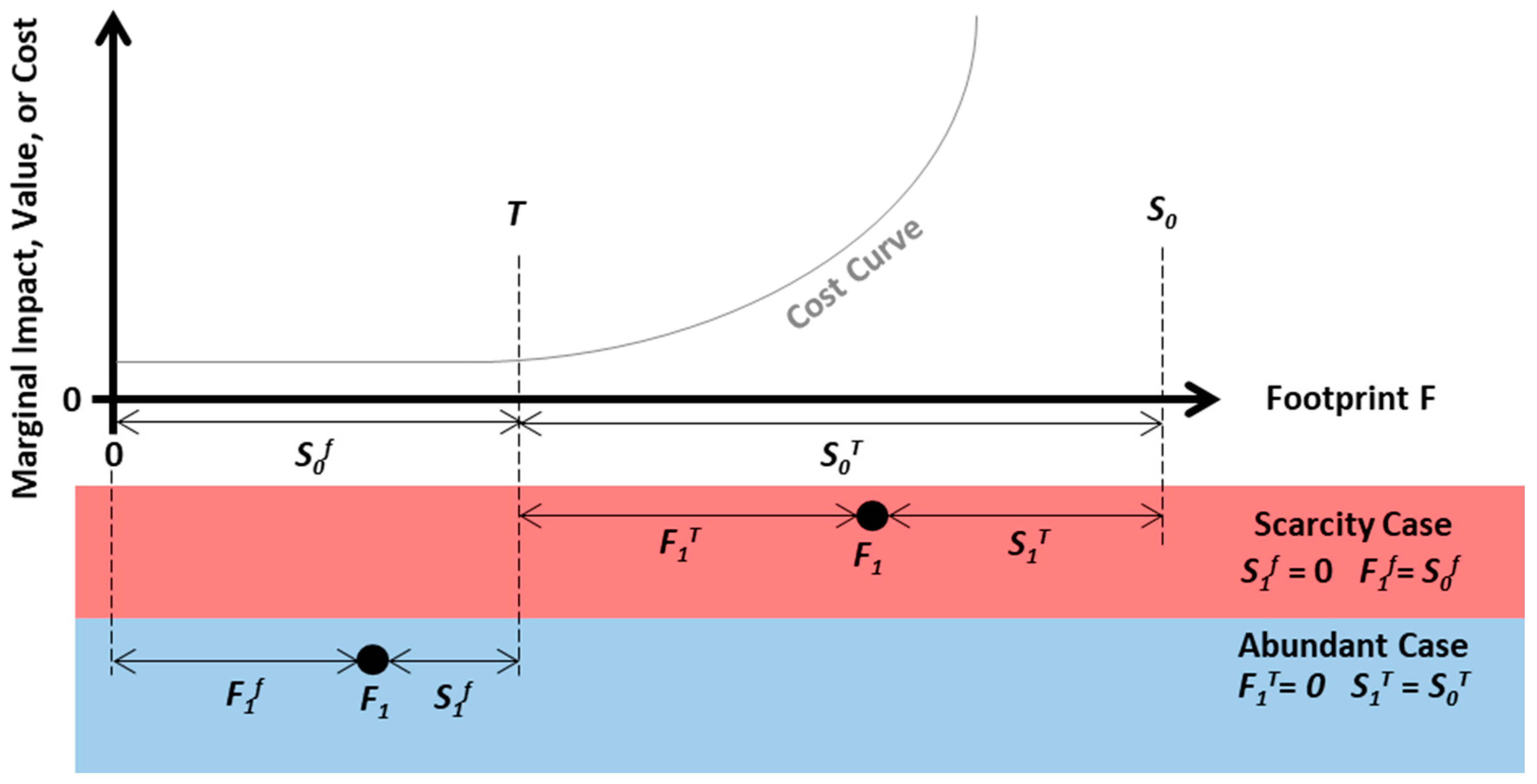
The aggregate net volumetric Footprint F is some fraction of W, adjusted by the withdrawal-weighted average consumption coefficient c of the processes, such that F = c W. F is also the Consumptive Use, in water applications. The Threshold-based Footprint FT is the nonnegative difference between F and the Threshold T (Equation (1), Figure 1). The stock’s Threshold is often a limit on the sustainable consumption or degradation of that stock. For example, an environmental flow requirement R would be the difference between the flow Q and the surface water stock’s threshold, such that R = Q − T. The Free Footprint Ff is the portion of F falling below the threshold T. This free portion of the footprint is discounted and characterized as having no impact because it has negligible environmental or economic cost (Equation (2), Figure 1). The relative Threshold T` = T/S is the Threshold expressed as a fraction of the Stock. Units of W, F, and T are those of S; c is unitless. If T = 0 then all resource withdrawals are adverse and FT = F; if T = S then all impacts are discounted and FT = 0. F = Ff until F > T. Observe in Equations (1) and (2) that the inventory of the stock S does not appear in the footprint calculation, but T does appear and is presumably related somehow to S. If FT = 0 the resource is “abundant” (negligible marginal value and cost), at least from the point of view of this decision making process. If FT > 0 the resource is scarce from the point of view of this decision making process and has non-negligible marginal value and cost.
F is the sum of the “free” and “adverse” components, such that F = FT + Ff. By definition, if c ≤ T`, then FT = 0 and F = Ff. The Free Fraction R of the footprint, R = Ff/F, is a sort of efficiency metric for the footprint. For example, if a river has a flow S of 1 Million m3/year and an adverse threshold T of 100,000 m3/year, and the total footprint F is 150,000 m3/year, then Ff = 100,000 m3/year and FT = 50,000 m3/year; R = 100,000/150,000 and thus two thirds of this footprint is “free”.
The initial adverse capacity above the threshold is S0T, where S0T = S0 − T0, and the initial free capacity below the threshold is S0f, where S0f = T0 (Figure 1). After an initial footprint F0 is applied, the remaining adverse capacity is S1T (Equation (3), Figure 1), and the remaining free capacity is S1f (Equation (4), Figure 1).
Fx is the footprint of an individual process x. Fx is not bounded by F when there are multiple processes, because the net impacts of different processes may be positive or negative and may offset, such that F = ∑x Fx. As with the aggregated footprint, the process’s footprint is the sum of the free and the adverse components, so Fx = FxT + Fxf. Processes may possess their own thresholds, Tx; a U.S. Environmental Protection Agency (EPA) regulation placing a Total Maximum Daily Load (TMDL) limit on a factory’s emission of water pollution is an example of a process having a threshold.
The relationship between the stock-level footprints and process-level footprints is complicated and is contextualized based on the policies governing this stock’s use. In a seniority-based framework such as the U.S. Western States’ Prior Appropriation Doctrine the first process to use water (x = 1), would have T1 = T. However, each subsequent and junior processes (x > 1) would have its threshold set at current free capacity of the stock, S1f (Equation (4)), after the sum total of all prior footprints F0 were deducted, such that F0 = ∑x_priorFx. Without any seniority one might choose to weight the threshold, free footprint, and adverse footprint of a process by its contribution to the footprint by using the weighting factor b = Fx/F, so FxT = b FT, Fxf = b Ff, and Tx = b T. Or, one could use a different weighting factor for a more progressive attribution system.
2.2. Application of the Threshold Concept to Water Footprints and Impact Metrics
The aggregated net consumptive fresh water use in the combined surface and ground water resources of a location is the “blue” Water Footprint (BWF). BWF is an implementation of F. The Threshold-based blue surface flow Water Footprint (TWF) is an implementation of FT. The Free Water Footprint (FWF) is equal to Ff. If BWF is used in LCA, it is an inventory, volumetric, or pressure type LCA metric, whereas TWF is a mid-point LCA metric. However, both use identical volumetric units, for instance cubic meters or gallons. Crucially, for example, for a company that seeks to measure the impact of its water footprint, for T > 0 it is not possible to calculate TWF or FWF without full knowledge of the net aggregated BWF of all other processes impacting that water stock, as well as the stock’s threshold. TWF and FWF therefore have a fundamentally higher burden of information than BWF.
The typical application of a Water Stress Index (WSI) [51] utilizes research concerning ecological water scarcity and flow variability at river basin and annual scales to characterize the impact of the consumptive freshwater use in the basin. In this paper [51] WSI is always defined as a logistic function of the stock-scale Withdrawal-to-Availability ratio (WTA) (Equation (5)), and is therefore a dimensionless fraction bounded below one. WSI* factors in low-flow season annual flow variability using a Variation Factor (VF), such that WSI* = WSI × VF. An empirically estimated median value for VF is 1.8 for annual-timescale river basin stock definitions [52,53]. If the river basin has a Strongly Regulated Flow (SRF) [53] due to a large reservoir storage capacity, WSI* becomes WSI*SRF where the square root of the VF is utilized, reflecting lower flow variability and less low-flow seasonal water stress in an SRF basin, such that WSI* = WSI × VF1/2. Note that this definition of WSI assumes a constant relationship between the WTA ratio and the water stress in the basin.
The Relevant for Environmental Deficiency metric (RED, Equation (19)) is a mid-point metric for the impact created by fresh water consumption at annual timescales for river basins [50], such that . The main mathematical difference between RED and TWF is that TWF varies the characterization of impact linearly following a discontinuity at the threshold, whereas RED uses a differentiable and smooth logistic characterization from WTA = 0. The main applied difference between TWF and RED as mid-point metrics is that regulations are typically written as thresholds, not smooth logistic functions—for better or worse. Implicit in the definition of RED is the existence of a complement to the characterized water impact, analogous to FWF. This is named Free from Environmental Deficiency (FED), such that FED = BWF − RED. These metrics, along with BWF, inform the ISO 14046 water LCA draft standard [54,55,56,57,58].
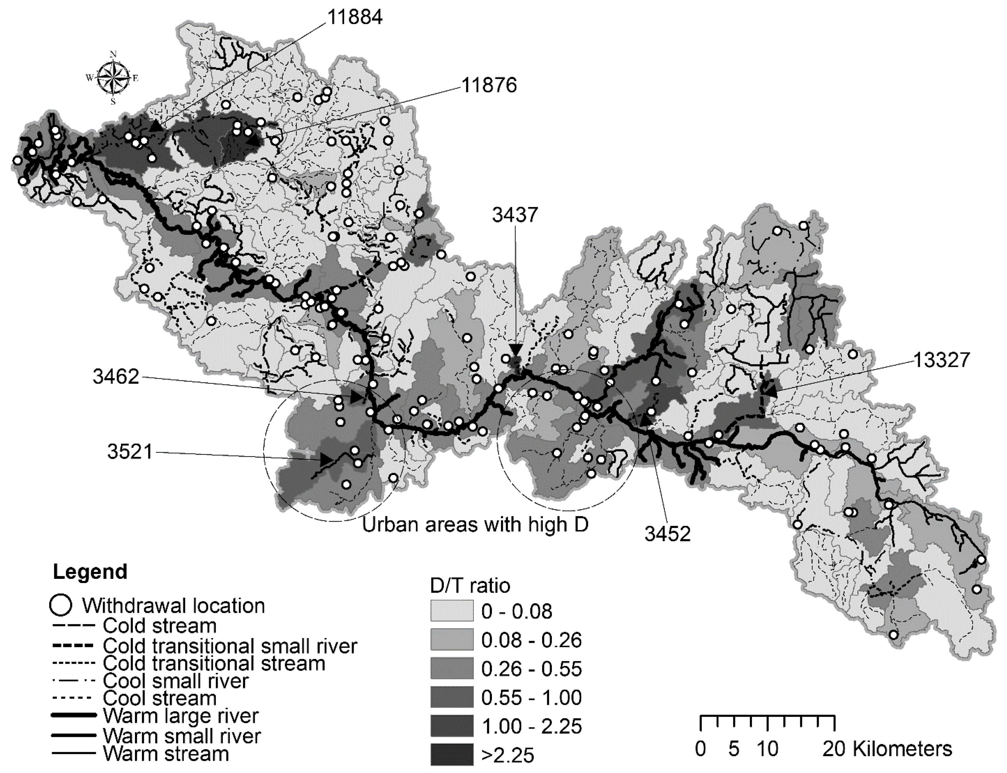
Similar mathematics have been applied in practice in prior case studies [59]. This study utilized flow depletion thresholds established by the State of Michigan’s Department of National Resources within that regulator’s Michigan Water Withdrawal Assessment Process (MWWAP) [60]. These thresholds are established uniquely for every individual stream segment in U.S. State of Michigan. Figure 2 reproduces that study’s map of the Kalamazoo River, where Mubako et al. [59] calculated the surface water flow Depletion, D, and compared it with the flow depletion threshold, T. Note that Mubako et al.’s [59] “D” is equivalent to F in this paper’s mathematics; it is the BWF calculated against the “stock” of surface water flow.
3. Results
To compare BWF, RED, FED, TWF, and FWF, a synthetic experiment is constructed for a theoretical stream flow. Imagine a stream with a flow of one cubic meter per second, giving initial capacity S0 = 1; hereafter these units will be omitted for simplicity so all results are unitless fractions of a river’s total flow. The experiment explores combinations of thresholds T`, consumption coefficients c, and Withdrawal-to-Availability (WTA) ratios, so that these five metrics can be compared side by side on a unitless basis. This comparison will make it clear that TWF can give quantitatively similar results to RED depending on the choice of threshold, and that the logistic form chosen by WSI implies an approximate “effective” threshold assumed by RED, a threshold that varies based on the combination of c and WTA.
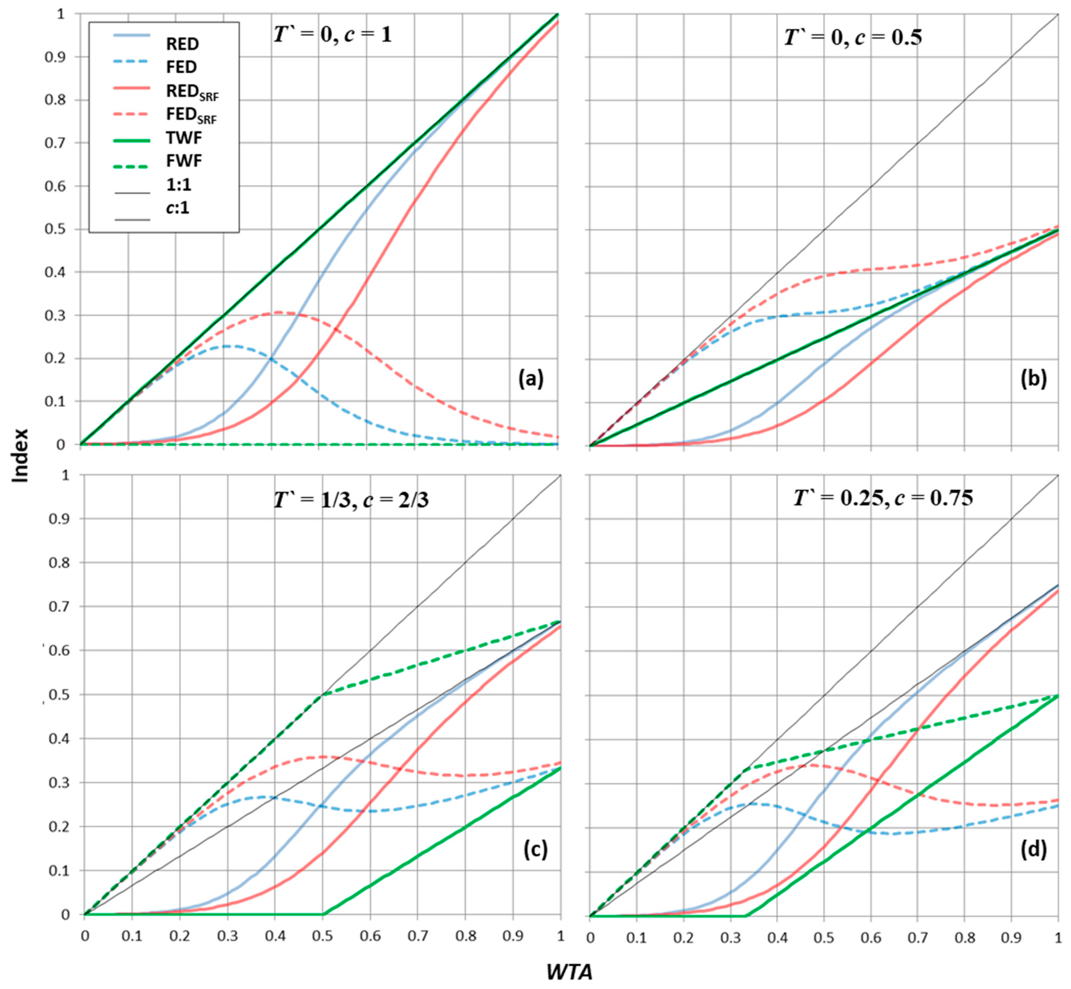
In Figure 3, the 1:1 line bounds all metrics and approximates FED and FWF for low WTA values that are far below the threshold. RED and TWF are bounded by the c:1 line; RED approaches this line as WTA → 1. TWF = 0 and BWF = FWF below the dimensionless value of WTA = T`/c. As a result, this dimensionless value defines a critical threshold for water sustainability policy, and it becomes clear that average consumption coefficients and thresholds are essential factors in this policy.
RED’s logistic form yields surprising dual peaks and local maxima in FED for higher consumptive use fractions (c = 0.6 to 0.9). This high range of consumptive use fractions is common in irrigation-dominated river basins, which are also often water stressed arid or semiarid warm-climate river basins. The smooth logistic function of RED can exceed a slope of one for moderate WTA and high c, meaning that an additional unit of withdrawal creates more than one unit of RED impact under these conditions. FED yields local maxima below the maximum-withdrawal point of WTA = 1 in many cases. These local maxima in FED are also local maxima in the Free Fraction R.
For a given c it is possible to calculate a threshold value T` that minimizes the difference between RED and TWF. This minimum-difference threshold can be considered the “effective” flow alteration threshold that is approximately implied by the form of RED and WSI. Best-fit T` is estimated for each c using a linear solver that minimizes the Root of the Mean Squared Error (RMSE) of the error function e = RED − TWF. Table 1 gives this best-fit T` for intervals of 0.1 (10%) of c for both the standard and SRF versions of RED. Also in Table 1 is given the RMSE value, the local maxima or “peak” value of FED, and the lowest WTA value at which a FED local maxima occurs.
The effective value of T` for RED ranges from 1% to 18%, rising with the assumed consumption coefficient. This range of values compares favorably with the river basin freshwater ecosystem flow requirement work [16,39] and specifically with the “presumptive standard” of less than 20% alteration of daily flow due to consumptive use [40], and with the MWWAP’s average threshold value of 10% depletion of median summer flows for streams in Michigan [59,60]. When this difference between RED and TWF is expressed relative to the size of the BWF, the relative difference (RMSE/c) is constant for all values of c, at 0.08 for the standard RED and 0.09 for the SRF variant of RED. These are relatively small errors that are less than 10% of the total water resource consumption in the system. It is therefore clear that TWF and RED are approximations of each other with a substantial quantitative and qualitative similarity.
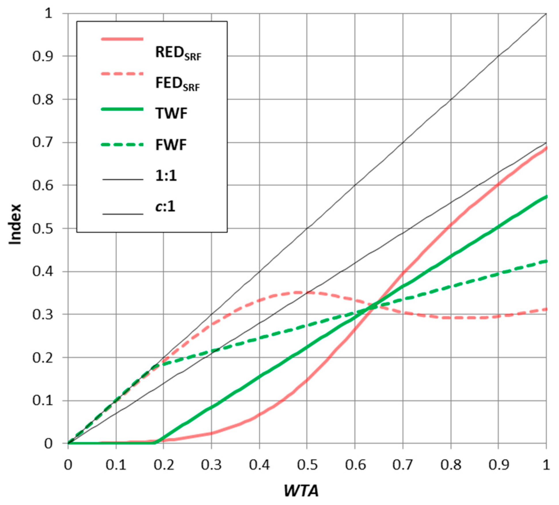
To complete the comparison, Figure 4 illustrates the best-fit relationship between RED and WSF. A typical consumptive use coefficient is c = 0.7 for heavily dammed, strongly-regulated, and heavily-utilized river basins dominated by irrigated agricultural water uses. This approximates the Lower Colorado River Basin in the United States, or the Nile River Basin below the Aswan dam in Egypt. The best fit between TWF and RED SRF in this case is T` = 0.125, or 12.5% of flow (Table 1, row in bold), a threshold that falls in the typical range published for ecological flow requirement thresholds [11,12,16,26,39,40]. Both RED and TWF mid-point impact indices visibly depart from zero at a threshold of approximately WTA = 0.18, have a shared value of approximately 0.33 when WTA = 0.63, and reach maxima near a value of 0.6 at WTA = 1. FED and FWF are also similar, although FWF monotonically increases whereas FED has a local maximum near WTA = 0.49. All four indexes are approximately equal when WTA = 0.63, and where Free Fraction R = 0.5 because TWF~FWF here. WTA = 0.63 is nearly the inflection point and maximum slope in RED, where the rate of change of impact per unit of water withdrawn switches from positive to negative. Relative to the size of the BWF, the difference between the two metrics is largest when WTA is in the range of 0.3 to 0.4, where TWF is roughly double RED. Figure 4 demonstrates that RED and TWF have quantitative and qualitative similarities, and are both somewhat lower than the c:1 line which delineates the equivalent BWF.
4. Discussion
Sustainability indexing is more difficult for some parts of the Coupled Natural–Human system than for others. Climate sustainability is relatively simple to assess using Carbon Footprints, because net emissions into a shared global atmosphere have no local context, and there is arguably a single global threshold for carbon dioxide in the atmosphere at around 400 ppm. Water lies at the most difficult extreme on a spectrum of natural resource types, because water resources are physically and ecologically complex, spatio-temporally variable, localized, politicized, regulated, publicly managed, culturally heterogeneous, and values-laden; water impacts are locally “context-based” [61,62]. Water scarcity and water stress is only one dimension of the complex local water context. Work to develop water sustainability indexes, performance indicators, and LCA methods has been difficult because it requires accurate and scale-specific empirically determined scientific knowledge of the system, and implicitly contains socio-political judgments regarding values and thresholds. This will also be true in many other sustainability applications of footprinting and LCA beyond water.
It is interesting to observe what information is required to calculate the quantities in equations one through seven. F and Fx can be calculated with knowledge of withdrawal and the consumption coefficient. FT, Ff, FxT, and Fxf require knowledge of the footprint and the threshold. The threshold T for the stock is obtained using external information which presumably includes reference to the initially available inventory of the stock, S0. However, the threshold Tx for an individual process, and by extension its adverse and free footprints, can only be calculated with external knowledge of seniority or weighting between processes, as well as the footprints of all processes. If F > T at the level of a stock, it is impossible to calculate an individual process’s Threshold-based Footprint FxT (a mid-point metric) without knowing the details of all the other processes’ footprints and thresholds, along with their weightings or priorities. If F < T (an abundant stock) it is known that FxT = 0 and Fxf = Fx, so the Blue Water Footprint of this individual process is sufficient information to calculate its mid-point impact. In other words, a factory or city or power plant needs to know the sum total of all other human and natural agents’ water uses and contributions (any significant uses that are upstream or sharing the water stock), along with the water stock’s adverse resource impact threshold, in order to calculate the impact of its own water use. In a system with seniority or priority the situation is even worse: each water user needs to know each other user’s water use and also each other user’s individual threshold and priority.
This information requirement for threshold-based accounting imposes a theoretical limitation with important real-world implications for water users and policymakers. It means that one of two solutions are probably needed to manage a water stock’s utilization rate and sustainability; either (1) large water users desiring to account for their water use impacts must take the lead on organizing watershed or aquifer level voluntary data sharing efforts, or (2) comprehensive top-down reporting and detailed public disclosure of (perhaps only large) water uses must be organized by a government or NGO. It is theoretically impossible for a company or city to calculate the impact of its water use without this detailed systemic data. This information requirement motivates costly systemic water data collection so that the more useful context-based mid-point impact metrics (e.g., TWF, WSF, RED) can be calculated. A Blue Water Footprint, by contrast, is easy for a company to calculate without any knowledge of other water users’ data- but this footprint is not locally contextualized. This finding highlights an important advantage of the simple inventory/volumetric approach taken by the standard Blue Water Footprint; it is currently much more feasible for an individual company or city to calculate their Blue Water Footprint than a mid-point impact metric like FxT, in the absence of systemic and publicly transparent water use and availability data.
Figure 3 and Figure 4 showed that the FED metric can yield local maxima below the maximum-withdrawal point of WTA = 1, owing to the nonlinear logistic form of WSI. This is an unexpected result that is either confounding or insightful depending on how much we trust the precise characterization of impact that is contained in WSI. If we trust the WSI characterization, we should perhaps steer policy toward achieving one of these local maxima in FED, because this would locally maximize the Free Fraction R and the (local) efficiency of water use patterns. However, these nonlinear local maxima are not present in the simpler, linear, and discontinuous mathematical form of FWF, which calls into question the robustness of such a maximization. Notably, no local maxima exist for the more important mid-point impact metrics RED or TWF, so policymakers may choose to ignore FED and FWF and rather simply minimize RED or TWF.
Resource thresholds and mid-point and end-point impact measurements depend on the decision maker’s point of view; in fact, even simple volumetric inventory metrics depend on point of view because external impacts may be correctly discounted [44,45]. In Figure 1, where would you choose to draw a sharp threshold that distinguishes “acceptable” impacts and costs from those that are unacceptably high? There are many methods and choices for T. TWF makes the choice explicit and visible. Because the use of the WSI characterization factor implies the acceptance of an approximate threshold value, the use of RED requires the acceptance of a specific—but implicit—point of view. This point of view is clearer now that we have an estimate for the thresholds that are implied by RED for each consumption coefficient. Fortunately, these results demonstrate that RED’s implicit thresholds range from 1% to 18% of the flow, which is totally compatible with best practices and presumptive standards for thresholds that are commonly held in heavily-managed and irrigation-dominated watersheds.
From the resource stock manager’s point of view, the objective is to minimize footprints and/or their social, environmental, and economic impacts [45]. When using Threshold-based Footprints, minimizing FT is the most urgent objective. This is accomplished by minimizing F, W, and c, but these metrics are equally dependent on Sf and T which can be relaxed through investment in infrastructure or manipulated by changing environmental laws and standards. Resource managers may also seek to maximize the Free Fraction R, or alternatively the ratio of “free” to “adverse” footprints. From the process manager’s differing point of view (e.g., as a company with a commitment to sustainability), the objective is to minimize this individual process’s adverse footprint FxT, which can be done either by reducing the process’s own footprint, or by offsetting that footprint by achieving reductions in another process’s footprint against the same resource stock.
In summary, this paper derives a mathematics for Threshold-based Footprints and develops a case study that compares the Blue Water Footprint (BWF), Threshold-based surface Water Footprint (TWF), and Relevant for Environmental Deficiency (RED) mid-point LCA impact metric. The findings are general and the Threshold-based Footprint metric is useful as an easily communicated and regulation-compatible “hybrid” between volumetric/inventory footprint metrics and LCA mid-point impact metrics. This new metric is directly applicable for context-based water management. Hopefully this simple threshold-based metric will make it easier to accurately and precisely account for impact in environmental systems that are governed by socio-economically influenced regulations, by harmonizing the impact metrics with the real-world regulations and environmental standards that govern these systems.
Funding
This work was made possible in part by the Great Lakes Protection Fund via Grant #946, by the U.S. Department of Energy’s Sandia National Laboratories, and by the U.S. National Science Foundation via the CAP-LTER grant (BCS-1026865), Water Sustainability and Climate grant (EAR-1360509), and INFEWS grant FEWSION (ACI-1639529). The findings are those of the authors, and not necessarily those of the funding agencies and partners.
Acknowledgments
Special thanks are extended to Alex Mayer and Stanley Mubako for their support of this work, and to the water resource professionals of the Great Lakes basin for their pioneering efforts to implement ecological flow thresholds into the scientific and regulatory framework of the region.
Conflicts of Interest
The author declare no conflict of interest.
Appendix A. Various Threshold-Based Water Scarcity and Stress Indices
Commonly employed scarcity and stress indices [35] may be expressed using these mathematics. The ratio of W to S (Equation (A1)) is identical to the commonly employed Withdrawal-to-Availability index (WTA) [47,48,49,50,51]. The ratio IC (Equation (A2))) of the aggregated footprint F to the Initial Capacity S is identical to the commonly employed Consumption-to-Availability scarcity index (CTA) [47]. Two alternative indices of scarcity are the Threshold-based Adverse Impact Index IT and the Threshold-based Free Impact Index If (EquationS (A3) and (A4)). The Threshold-based Scarcity Index I, is the ratio of the total footprint to the threshold (Equation (A5)), such that the stock is in a “scarce” condition when F > T and the critical value of the dimensionless number is 1. The proportion of the aggregated net footprint that is adverse is PT, and the free proportion is Pf (Equations (A5) and (A6)). The Free Impact Ratio RI is the ratio of free to adverse impacts, R = Ff/FT (Equation (A7)). Many other straightforward combinations of these metrics are possible.
Process-specific indices may be constructed. For example, the process’s fraction of FT is the Process-level Scarcity Footprint Fraction, PxT (Equation (A8)). Similarly, the process’s fraction of Ff is the Process-level Free Footprint Fraction, Pxf, and the process’s fraction of F is the Process-level Footprint Fraction, Px
Appendix B. The Economic Interpretation of FT
Sustainability indexing methods for have been criticized for ignoring economics. In the case of the Water Footprint, for example, the key criticism is that that water has a differing value depending on the place and time of its consumption [63,64]. Therefore, a volumetric Water Footprint cannot be applied uniformly in all locations as a sustainability impact metric, because a unit volume of water consumption could have a large impact in one case and zero impact in another case. We address this criticism by discounting the volumetric impacts below a threshold of “scarcity”, and interpreting FT as an index for the total cost of net aggregated impacts. Water Scarcity Footprints attempt to address this limitation by indexing for the economic condition of scarcity, without attempting to directly address the value of the resource [35,65]. A threshold-based footprint fits this general category.
In what sense is a threshold-based footprint an index of scarcity? In this case “Scarcity” means that there is competition for the stock, and that not all demands can be satisfied at a near-zero (shadow) price. The existence of scarcity implies that some sort of impact is occurring in the system, and that the stock is a “rival” resource [45]. Scarcity is the opposite of “abundance”, where no impact or cost is perceived in the system. Scarcity is a normal condition in formal markets, but is a relatively novel condition for most environmental and natural resource management scenarios (especially water), because the responsible human institutions have evolved to prevent water scarcity on the margin (at best) or to imagine that it does not exist (at worst), for example, for water [30,66].
Scarcity footprints exists at specific locations in space and time, and can only be perceived if the spatio-temporal boundaries of the stock r are properly defined [44,67,68]. The Marginal Opportunity Cost of a single additional unit of net impact on a resource stock is illustrated using the Cost Curve in Figure 1. The Opportunity Cost is usually understood as the benefit gained from the most valuable possible alternative application of that resource. In Figure 1 it is clear that the Cost Curve begins with a value near zero and steadily increases as total impacts increase, until at some point the Opportunity Cost is very high or possibly undefined (i.e., the resource is then marginally “priceless”) at the point where aggregated net impact Fr on the stock equals the initial capacity S of the stock. The Adverse Impact Threshold for this specific stock T is chosen at the highest value of F where the Opportunity Cost is close enough to zero to be “acceptable” in some socio-environmental-political value judgment. The stock is considered to be “scarce” with adverse marginal impacts and unacceptably high marginal costs when F > T, and the stock is “abundant” when F < T. Multiple cost curves and thresholds may exist for different types of impacts; in this case, the lowest T should typically be chosen. In the case where water LCA assesses impacts on a sensitive wetland, the acceptable impact threshold might be close to zero [69]. For a nonrenewable resource that is subject to market pricing, this threshold will usually be zero.
We have therefore introduced with the threshold based footprint a sustainability metric that is simultaneously an index for the economic concept of marginal value and scarcity, such that these are zero below the scarcity threshold, and above the scarcity threshold the marginal value is fixed at a single value. This approximation is excellent when F ≤ T (an ‘abundant’ stock where impacts are relatively free of cost), and is generally valid for F << S (a stock not under extreme stress). The total aggregated price (or value) of the resource’s utilization is in proportion to the ratio of the threshold to the total cumulative stock impacts, T/F (the ratio is bounded at zero and one). If T = 0 there is no discount, and if F < T, the discount is 100%. Between these two points, the total aggregated price scales linearly. If T = S, all impacts on the stock are 100% discounted. T = 0 would occur for a nonrenewable imperishable resource stock such as gold, and T = S might occur for a perishable resource that has only one possible use such as water in an agricultural irrigation system (i.e., a “use-it-or-lose-it” resource).
The shape of the cost curve should have a strong empirical economic basis, but the precise location of the threshold is necessarily informed by subjective and socio-politically contextual judgments as to what is ‘acceptable’ versus what is ‘adverse’. Adverse resource impact thresholds integrate ecology and the subjective socio-environmental-political politics of value, cost, and impact [12,58].
References
- Liu, J.; Dietz, T.; Carpenter, S.R.; Folke, C.; Alberti, M.; Redman, C.L.; Schneider, S.H.; Ostrom, E.; Pell, A.N.; Lubchenco, J.; et al. Coupled human and natural systems. Ambio 2007, 36, 639–649. [Google Scholar] [CrossRef]
- Cohen, S. We Need to Accelerate the Development of Sustainability Metrics. Available online: https://www.whu.edu/en/faculty-research/entrepreneurship-and-innovation-group/chair-of-entrepreneurship-i/sustainability-blog/measuring-sustainability-the-need-for-precise-metrics/ (accessed on 30 July 2018).
- Marten, S.; Carpenter, S.R.; Lenton, T.M.; Bascompte, J.; Brock, W.; Dakos, V.; van de Koppel, J.; van de Leemput, I.A.; Levin, S.A.; van Nes, E.H; et al. Anticipating critical transitions. Science 2012, 338, 344–348. [Google Scholar]
- Walker, B.; Holling, C.S.; Carpenter, S.R.; Kinzing, A. Resilience, adaptability, and transformability in socio-ecological systems. Ecol. Soc. 2004, 9, 5. [Google Scholar] [CrossRef]
- RA/SFI. Thresholds and Alternate States in Ecological and Social–Ecological Systems; Resilience Alliance report #183; Resilience Alliance and Santa Fe Institute: Santa Fe, NM, USA, 2009. [Google Scholar]
- Couttenier, M.; Soubeyran, R. Drought and Civil War in Sub-Saharan Africa; Working Paper no.21; Paris School of Economics: Paris, France, 2011. [Google Scholar]
- Duarte, C.M.; Agusti, S.; Agawin, N.S.R. Response of a Mediterranean phytoplankton community to increased nutrient inputs: A mesocosm experiment. Mar. Ecol. Prog. Ser. 2000, 195, 61–70. [Google Scholar] [CrossRef]
- Solimini, A.G.; Cardoso, A.C.; Heiskanen, A.-S. Indicators and Methods for the Ecological Status Assessment under the Water Framework Directive; #EUR-22314-EN; European Commission Joint Research Centre Institute for Environment and Sustainability: Ispra, Italy, 2006. [Google Scholar]
- Lawn, P.A. An assessment of the valuation methods used to calculate the Index of Sustainable Economic Welfare (ISEW), Genuine Progress Indicator (GPI), and Sustainable Net Benefit (SNBI). Environ. Dev. Sustain. 2005, 7, 185–208. [Google Scholar] [CrossRef]
- Wang, L.Z.; Lyons, J.; Kanehl, P. Impacts of urbanization on stream habitat and fish across multiple spatial scales. Environ. Manag. 2001, 28, 255–266. [Google Scholar] [CrossRef]
- Steinman, A.D.; Nicholas, J.R.; Seelbach, P.W.; Allan, J.W.; Ruswick, F. Science as a fundamental framework for shaping policy discussions regarding the use of groundwater in the State of Michigan: A case study. Water Policy 2011, 13, 69–86. [Google Scholar] [CrossRef]
- Reeves, H.W.; Hamilton, D.A.; Seelbach, P.W.; Asher, A.J. Ground-Water-Withdrawal Component of the Michigan Water-Withdrawal Screening Tool; United States Geological Survey Scientific Investigations Report 2009–5003; United States Geological Survey: Reston, VA, USA, 2009; p. 36.
- Swartz, W.; Sala, E.; Tracey, S.; Watson, R.; Pauly, D. The Spatial Expansion and Ecological Footprint of Fisheries (1950 to Present). PLoS ONE 2010, 5, e15143. [Google Scholar] [CrossRef] [PubMed]
- EPA. Clean Water Act Sec. 303(d), 33 U.S.C. § 1313(d); EPA: Washington, DC, USA, 1972. [Google Scholar]
- EPA. Water Quality Planning and Management; Code of Federal Regulations, 40 CFR 130.7.; EPA: Washington, DC, USA, 1992. [Google Scholar]
- Richter, B.D.; Mathews, R.; Harrison, D.L.; Wigington, R. Ecologically sustainable water management: Managing river flows for ecological integrity. Ecol. Appl. 2003, 13, 206–224. [Google Scholar] [CrossRef]
- Sayre, N.F. The Genesis, History, and Limits of Carrying Capacity. Ann. Assoc. Am. Geogr. 2008, 98, 120–134. [Google Scholar] [CrossRef]
- Rees, W.E.; Wackernagel, M. Ecological Footprints and Appropriated Carrying Capacity: Measuring the Natural Capital Requirements of the Human Economy; Jansson, A., Folke, C., Hammer, M., Costanza, R., Eds.; Island Press: Washington, DC, USA, 1994. [Google Scholar]
- Ehrlich, P.R.; Holdren, J.P. Impact of Population Growth. Science 1971, 171, 1212–1217. [Google Scholar] [CrossRef] [PubMed]
- Yang, H.; Reichert, P.; Abbaspour, K.C.; Zehnder, A.J.B. A water resources threshold and its implications for food security. Environ. Sci. Technol. 2003, 37, 3048–3054. [Google Scholar] [CrossRef] [PubMed]
- Galli, A.; Wiedmann, T.; Ercin, E.; Knoblauch, D.; Ewing, B.; Giljum, S. Integrating Ecological, Carbon and Water footprint into a “Footprint Family” of indicators: Definition and role in tracking human pressure on the planet. Ecol. Indic. 2012, 16, 100–112. [Google Scholar] [CrossRef]
- Perez-Dominguez, R.; Maci, S.; Courrat, A.; Borja, A.; Neto, J.; Elliott, M. Review of Fish-Based Indices to Assess Ecological Quality Condition in Transitional Waters; Available online: http://www.wiser.eu/download/D4.4-1.pdf (accessed on 30 July 2018).
- Zhang, Y.; Singh, S.; Bakshi, B.R. Accounting for ecosystem services in life cycle assessment, Part I: A critical review. Environ. Sci. Technol. 2010, 44, 2232–2242. [Google Scholar] [CrossRef] [PubMed]
- Fiksel, J.; Bruins, R.; Gatchett, A.; Gilliland, A.; Ten Brink, M. The triple value model: A systems approach to sustainable solutions. Clean Technol. Environ. Policy 2014, 16, 691–702. [Google Scholar] [CrossRef]
- Palmer, M.A.; Lettenmaier, D.P.; Poff, N.L.; Postel, S.L.; Richter, B.; Warner, R. Climate change and river ecosystems: Protection and adaptation options. Environ. Manag. 2009, 44, 1053–1068. [Google Scholar] [CrossRef] [PubMed]
- Poff, N.L.; Richter, B.D.; Arthington, A.H.; Bunn, S.E.; Naiman, R.J.; Kendy, E.; Acreman, M.; Apse, C.; Bledsoe, B.P.; Freeman, M.C.; et al. The ecological limits of hydrologic alteration (ELOHA): A new framework for developing regional environmental flow standards. Freshw. Biol. 2010, 55, 147–170. [Google Scholar] [CrossRef]
- Postel, S.; Richter, B.D. Rivers for Life: Managing Water for People and Nature; Island Press: Washington, DC, USA, 2003; ISBN 978-1559634441. [Google Scholar]
- Witmer, M.C.H.; Cleij, P. Water Footprint: Useful for Sustainability Policies; #500007001; PBL Netherlands Environmental Assessment Agency: The Hague, The Netherlands, 2012. [Google Scholar]
- Tharme, R.E. A global perspective on environmental flow assessment: Emerging trends in the development and application of environmental flow methodologies for rivers. River Res. Appl. 2003, 19, 397–442. [Google Scholar] [CrossRef]
- Postel, S.L. Entering an Era of Water Scarcity: The Challenges Ahead. Ecol. Appl. 2000, 10, 941–948. [Google Scholar] [CrossRef]
- Hoekstra, A.Y.; Wiedmann, T.O. Humanity’s unsustainable environmental footprint. Science 2014, 344, 1114–1117. [Google Scholar] [CrossRef] [PubMed]
- Falkenmark, M. Water and sustainability: A reappraisal. Environment 2008, 50, 4–16. [Google Scholar] [CrossRef]
- Meadows, D.H.; Meadows, D.H.; Randers, J.; Behrens, W.W., III. The Limits to Growth: a report to the Club of Rome. Available online: http://www.donellameadows.org/wp-content/userfiles/Limits-to-Growth-digital-scan-version.pdf (accessed on 30 July 2018).
- Hussen, A. Principles of Environmental Economics and Sustainability: An Integrated Economic and Ecological Approach, 3rd ed.; Routledge: Abingdon, UK, 2012. [Google Scholar]
- Brown, A.; Matlock, M.D. A Review of Water Scarcity Indices and Methodologies. White Pap. 2011, 106, 19. [Google Scholar]
- Gini, C. Variabilità e mutabilità. In Memorie di Metodologica Statistica; Pizetti, E., Salvemini, T., Eds.; Libreria Eredi Virgilio Veschi: Rome, Italy, 1955. [Google Scholar]
- Jackson, L.E.; Kurtz, J.C.; Fisher, W.S. Evaluation Guidelines for Ecological Indicators; #EPA/620/R-99/005; U.S. Environmental Protection Agency: Washington, DC, USA, 2000.
- Samhouri, J.F.; Levin, P.S.; Ainsworth, C.H. Identifying Thresholds for Ecosystem-Based Management. PLoS ONE 2010, 5, e8907. [Google Scholar] [CrossRef] [PubMed]
- Richter, B.D.; Warner, A.T.; Meter, J.L.; Lutz, K. A collaborative and adaptive process for developing environmental flow recommendations. River Res. Appl. 2006, 22, 297–318. [Google Scholar] [CrossRef]
- Richter, B.D.; Davis, M.M.; Apse, C.; Konrad, C. A presumptive standard for environmental flow protection. River Res. Appl. 2012, 28, 1312–1321. [Google Scholar] [CrossRef]
- Wiedmann, T.; Barrett, J. A Review of the Ecological Footprint Indicator—Perceptions and Methods. Sustainability 2010, 2, 1645–1693. [Google Scholar] [CrossRef] [Green Version]
- Solanes, M.; Gonzalez-Villarreal, F. The Dublin Principles for Water as Reflected in a Comparative Assessment of Institutional and Legal Arrangements for Integrated Water Resources Management; Global Water Partnership: Stockholm, Sweden, 1999. [Google Scholar]
- Glennon, R. Unquenchable; Island Press: Washington, DC, USA, 2010. [Google Scholar]
- Ruddell, B.L.; Adams, E.A.; Rushforth, R.; Tidwell, V.C. Embedded resource accounting for coupled natural-human systems: An application to water resource impacts of the western US electrical energy trade. Water Resour. Res. 2014, 50, 7957–7972. [Google Scholar] [CrossRef]
- Rushforth, R.R.; Adams, E.A.; Ruddell, B.L. Generalizing ecological, water and carbon footprint methods and their worldview assumptions using Embedded Resource Accounting. Water Resour. Ind. 2013, 1, 77–90. [Google Scholar] [CrossRef]
- Kates, R.W.; Clark, W.C.; Corell, R.; Hall, J.M.; Jaeger, C.C.; Lowe, I.; McCarthy, J.J.; Schellnhuber, H.J.; Bolin, B.; Dickson, N.M.; et al. Sustainability Science. Science 2001, 292, 641–642. [Google Scholar] [CrossRef] [PubMed]
- Berger, M.; Finkbeiner, M. Water footprinting: How to address water use in life cycle assessment? Sustainability 2010, 2, 919–944. [Google Scholar] [CrossRef]
- Berger, M.; Finkbeiner, M. Methodological Challenges in Volumetric and Impact-Oriented Water Footprints. J. Ind. Ecol. 2012, 17, 79–89. [Google Scholar] [CrossRef]
- Hoekstra, A.Y.; Chapagain, A.K.; Aldaya, M.M.; Mekonnen, M.M. The Water Footprint Assessment Manual: Setting the Global Standard; Water Footprint Network; Earthscan Publishing: Oxford, UK, 2011. [Google Scholar]
- Pfister, S.; Bayer, P.; Koehler, A.; Hellweg, S. Environmental Impacts of Water Use in Global Crop Production: Hotspots and Trade-Offs with Land Use. Environ. Sci. Technol. 2011, 45, 5761–5768. [Google Scholar] [CrossRef] [PubMed]
- Pfister, S.; Koehler, A.; Hellweg, S. Assessing the environmental impacts of freshwater consumption in LCA. Environ. Sci. Technol. 2009, 43, 4098–4104. [Google Scholar] [CrossRef] [PubMed]
- Nilsson, C.; Reidy, C.A.; Dynesius, M.; Revenga, C. Fragmentation and flow regulation of the world’s large river systems. Science 2005, 308, 405–408. [Google Scholar] [CrossRef] [PubMed]
- Ridoutt, B.; Pfister, S. A revised approach to water footprinting to make transparent the impacts of consumption and production on global freshwater scarcity. Glob. Environ. Chang. 2010, 20, 113–120. [Google Scholar] [CrossRef]
- Chenoweth, J.; Hadjikakou, M.; Zoumides, C. Review article: Quantifying the human impact on water resources: A critical review of the water footprint concept. Hydrol. Earth Syst. Sci. Discuss. 2013, 10, 9389–9433. [Google Scholar] [CrossRef]
- Kounina, A.; Margni, M.; Bayart, J.; Boulay, A.; Berger, M.; Bulle, C.; Frischknecht, R.; Koehler, A.; Mila i Canals, L.; Motoshita, M.; et al. Review of methods addressing freshwater use in life cycle inventory and impact assessment. Int. J. Life Cycle Assess. 2013, 18, 707–721. [Google Scholar] [CrossRef]
- Mila i Canals, L.; Chenoweth, J.; Chapagain, A.; Orr, S.; Anton, A.; Clift, R. Assessing freshwater use in LCA: Part I—Inventory modelling and characterization factors for the main impact pathways. Int. J. Life Cycle Assess. 2008, 14, 28–42. [Google Scholar] [CrossRef]
- Pfister, S.; Ridoutt, B.G. Water footprint: Pitfalls on common ground. Environ. Sci. Technol. 2013, 48, 4. [Google Scholar] [CrossRef] [PubMed]
- ISO (2014), ISO 14046:2014(en): Environmental Management—Water Footprint—Principles, Requirements and Guidelines. Available online: https://www.iso.org/obp/ui/#iso:std:iso:14046:ed-1:v1:en (accessed on 30 July 2018).
- Mubako, S.T.; Ruddell, B.L.; Mayer, A.S. Relationship between water withdrawals and freshwater ecosystem water scarcity quantified at multiple scales for a Great Lakes watershed. J. Water Resour. Plan. Manag. 2013, 139, 671–681. [Google Scholar] [CrossRef]
- Zorn, T.G.; Seelbach, P.W.; Rutherford, E.S.; Wills, T.C.; Cheng, S.T.; Wiley, M.J. A Regional-Scale Habitat Suitability Model to Assess the Effects of Flow Reduction on Fish Assemblages in Michigan Streams; Fisheries Research Report 2089; Michigan Department of Natural Resources: Ann Arbor, MI, USA, 2008. [Google Scholar]
- Pacific Institute. Exploring the Case for Corporate Context-Based Water Targets. 2017. Available online: https://www.ceowatermandate.org/files/context-based-targets.pdf (accessed on 28 June 2018).
- Alliance for Water Stewardship. The AWS International Water Stewardship Standard. 2014. Available online: http://a4ws.org/wp-content/uploads/2017/04/AWS-Standard-Full-v-1.0-English.pdf (accessed on 28 June 2018).
- Wichelns, D. Virtual water and water footprints offer limited insight regarding important policy questions. Int. J. Water Resour. Dev. 2010, 26, 639–651. [Google Scholar] [CrossRef]
- Hanemann, W.M. Chapter 4: The economic conception of water. In Water Crisis: Myth or Reality; Rogers, P.P., Llamas, M.R., Martinez-Cortina, L., Eds.; Taylor & Francis Group: Oxford, UK, 2006; pp. 61–91. [Google Scholar]
- Hoekstra, A.Y.; Mekonnen, M.M.; Chapagain, A.K.; Mathews, R.E.; Richter, B.D. Global monthly water scarcity: Blue water footprints versus blue water availability. PLoS ONE 2012, 7, e32688. [Google Scholar] [CrossRef] [PubMed]
- Zetland, D. The End of Abundance: Economic Solutions to Water Scarcity; Aguanomics Press: Mission Viejo, CA, USA, 2011; ISBN 978-0615469737. [Google Scholar]
- Fang, K.; Heijungs, R.; de Snoo, G.R. Understanding the complementary linkages between environmental footprints and planetary boundaries in a footprint–boundary environmental sustainability assessment framework. Ecol. Econ. 2015, 114, 218–226. [Google Scholar] [CrossRef]
- Heistermann, M. HESS Opinions: A planetary boundary on freshwater use is misleading. Hydrol. Earth Syst. Sci. 2017, 21, 3455–3461. [Google Scholar] [CrossRef] [Green Version]
- Verones, F.; Pfister, S.; Hellweg, S. Quantifying Area Changes of Internationally Important Wetlands Due to Water Consumption in LCA. Environ. Sci. Technol. 2013, 47, 9799–9807. [Google Scholar] [CrossRef] [PubMed]
Figure 1.
Schematic of the Threshold-based Footprint concept. The vertical axis gives the marginal value, impact or cost of water use, and the horizontal axis gives the Footprint. The cost of the footprint increases slowly at first as the footprint rises, but beyond a threshold it increases sharply and in unbounded fashion as the resource becomes “scarce” and the marginal value, impact, and cost begin to rise. Illustrations of footprint components during “scarcity” (F > T) and “abundant” (F ≤ T) conditions are given. Section 2.1 defines mathematical symbols and equations. Commonly employed scarcity and stress indices [35] may be expressed using these mathematics (Appendix A). A discussion of the interpretation of impact and cost is provided in Appendix B.

Figure 2.
Ratio of the surface water flow (Blue) Water Footprint (BWF = D = FT) to the streamflow depletion threshold, T, for each stream segment of the Kalamazoo River in Michigan, USA. Dark grey colors where D/T > 1 indicate the presence of scarcity where FT > 0. This is Figure 5 [59] reproduced with permission of ASCE Press and the Authors.

Figure 3.
Comparisons between the Relevant for Environmental Deficiency (RED) midpoint impact indicator (in red, with RED Strongly Regulated Flow (SRF) version in blue) and Threshold-based Water Footprint (TWF) (in green), with different choices of threshold T` and mean consumptive use coefficient c, plotted against the Withdrawal-to-Availability index (WTA). BWF is coincident with the c:1 line and bounds RED and TWF. (a) T` = 0, c = 1: “Simple Withdrawal” case where all withdrawn water is consumed and counts as adverse impact, resulting in large differences between RED and TWF and additionally Free Water Footprint (FWF) = 0. (b) T` = 0, c = 0.5: “Symmetry” case resulting in a symmetry of RED and Free from Environmental Deficiency (FED) metrics about TWF and FWF, bounding of TWF and FWF by RED and FED, and TWF = FWF. (c) T` = 1/3, c = 2/3; “Reversal” case where RED → FWF and TWF → FED as WTA → 1, and TWF = 0 when WTA < 0.5. (d) T` = 0.25, c = 0.75; “Convergence” case where TWF converges to FWF at WTA = 1, and RED and FED metrics are bounded by TWF and FWF below WTA = 0.58.

Figure 4.
Water impact indices for the SRF irrigation-dominated best-fit special case where T` = 0.125 and c = 0.7. Note the similarity between RED SRF, in red, and TWF, in green. RED SRF and TWF are approximately equal below WTA = 0.20 and at WTA = 0.63. BWF is coincident with the c:1 line, and is somewhat higher than RED and TWF.


Table 1.
The effective flow alteration thresholds T` that are approximately implied by RED range from 1% to 18% depending on the details. Table gives values of T` that are the best-fit between RED and TWF, for each consumptive use coefficient (increments of 0.1), achieved by varying T` and WTA. Also shown is the Root Mean Squared Error (RMSE) of fit and the local-maxima or peak value of FED.
| RED | RED SRF | |||||||||
|---|---|---|---|---|---|---|---|---|---|---|
| c | T` | RMSE | Peak FED | @ WTA | Notes | T` | RMSE | Peak FED | @ WTA | Notes |
| 0 | - | 0 | 1 | 1 | - | 0 | 1 | 1 | ||
| 0.1 | 0.010 | 0.008 | 0.900 | 1 | 0.018 | 0.009 | 0.902 | 1 | ||
| 0.2 | 0.019 | 0.016 | 0.800 | 1 | 0.036 | 0.018 | 0.804 | 1 | ||
| 0.3 | 0.029 | 0.024 | 0.700 | 1 | 0.054 | 0.027 | 0.705 | 1 | ||
| 0.4 | 0.038 | 0.032 | 0.600 | 1 | 0.071 | 0.036 | 0.607 | 1 | ||
| 0.5 | 0.048 | 0.040 | 0.500 | 1 | 0.089 | 0.045 | 0.509 | 1 | ||
| 0.6 | 0.058 | 0.048 | 0.401 | 0.4 | FED local maxima | 0.107 | 0.054 | 0.411 | 0.54 | FED local maxima |
| 0.7 | 0.067 | 0.056 | 0.301 | 0.37 | FED local maxima | 0.125 | 0.064 | 0.351 | 0.49 | FED local maxima |
| 0.8 | 0.077 | 0.064 | 0.248 | 0.34 | FED local maxima | 0.143 | 0.073 | 0.333 | 0.46 | FED local maxima |
| 0.9 | 0.086 | 0.072 | 0.238 | 0.33 | FED local maxima | 0.161 | 0.082 | 0.319 | 0.44 | |
| 1 | 0.096 | 0.080 | 0.228 | 0.31 | 0.179 | 0.091 | 0.306 | 0.42 | ||
| 1 | 0.000 | 0.122 | 0.228 | 0.31 | 0.000 | 0.190 | 0.306 | 0.42 | ||
| RMSE/c = 0.08 | RMSE/c = 0.09 | |||||||||
© 2018 by the author. Licensee MDPI, Basel, Switzerland. This article is an open access article distributed under the terms and conditions of the Creative Commons Attribution (CC BY) license (http://creativecommons.org/licenses/by/4.0/).
Share and Cite
MDPI and ACS Style
Ruddell, B.L. Threshold Based Footprints (for Water). Water 2018, 10, 1029. https://doi.org/10.3390/w10081029
AMA Style
Ruddell BL. Threshold Based Footprints (for Water). Water. 2018; 10(8):1029. https://doi.org/10.3390/w10081029
Chicago/Turabian StyleRuddell, Benjamin L. 2018. "Threshold Based Footprints (for Water)" Water 10, no. 8: 1029. https://doi.org/10.3390/w10081029
Note that from the first issue of 2016, this journal uses article numbers instead of page numbers. See further details here.