Evaluating Energy and Cost Requirements for Different Configurations of Off-Grid Rainwater Harvesting Systems


1
Department of Physics, University of Texas at Austin, Austin, TX 78712, USA
2
Department of Mechanical Engineering, University of Texas at Austin, Austin, TX 78712, USA
3
Energy Institute, University of Texas at Austin, Austin, TX 78712, USA
*
Author to whom correspondence should be addressed.
Water 2018, 10(8), 1024; https://doi.org/10.3390/w10081024
Submission received: 31 March 2018
/
Revised: 11 July 2018
/
Accepted: 26 July 2018
/
Published: 2 August 2018
(This article belongs to the Special Issue Energy Efficient Management of Water Collection, Treatment, Storage and Distribution)
Abstract
:The goal of this analysis was to evaluate energy and cost requirements for different configurations of a rainwater harvesting (RWH) system in conjunction with a solar PV and energy storage system for an off-grid house. Using models in fluid mechanics, we evaluated energy and power requirements for four different system configurations: 1. An On-Demand System containing a single speed pump (OD-SS), 2. An On-Demand System containing a variable speed pump (OD-VS), 3. A Pressurized Storage System where water is pumped once during the day into a large pressurized tank for later consumption and treated on demand via UV light (PS-AOT), and 4. A Pressurized Storage System where water is treated once per day via UV light and then stored for later consumption (PS-TO). Our analysis showed that the OD-SS system model requires 2.63 kWh per day, the OD-VS system model requires a total energy of 1.65 kWh per day, and the PS-AOT requires 1.67–1.69 kWh per day depending on the pump size, and the PS-TO system requires 0.19–0.36 kWh per day depending on the pump size. When comparing estimated cost between systems, we found the OD-SS system to be the most expensive. With the OD-SS system as a base for system costs, we found the OD-VS system to be 39% less expensive, the PS-AOT system to be 21% less expensive, and the PS-TO system to be 60% less expensive than the base OD-SS system.
1. Introduction
Increasing water scarcity around the U.S. and the world has sparked interest in alternative water supplies and auxiliary water systems, including rainwater harvesting (RWH) for both potable and non-potable use [1]. Improvements in design standards of first flush diverters, ceramic filters, and pressurized storage tanks have enabled the use of RWH systems as supplemental sources for irrigation and even drinking water. Emerging technologies such as UV light treatment has made harvested rainwater a viable source for potable residential water supply [2].
A reliable potable water system is a critical component of modern living. For homeowners with off-grid houses, providing reliable potable water also requires a reliable electricity supply to run the pump(s) and treatment system. According to the Environmental Protection Agency, approximately 15% of Americans rely on private water wells for drinking water [3]. Over the next 50 years, we might see more off-grid residents building PV-powered (or solar powered) water systems around the world.
When it comes to designing PV-powered off-grid water systems, there is the question of how much power and energy are required to treat and deliver pressurized water for use throughout the day and night. These variables are important because they impact the sizing of the PV array and battery storage, both of which can be expensive. This work is motivated by the idea that water storage, which is typically affordable, could serve as a proxy for battery storage, thereby reducing overall costs. Batteries, while coming down in price, are still a major cost for off-grid systems. This paper aims to answer the question: Can altering the configuration of an off-grid rainwater system save energy and reduce system power demand while lowering the cost of an off-grid system?
There have been several studies relating energy requirements and RWH systems. For example, studies have looked into how residential and commercial RWH systems compare in energy intensity with conventional town water supply systems, and how startup energy can contribute to higher than anticipated energy requirements [4,5]. In addition, there have been studies on the life cycle analyses of the operational energy contribution for RWH systems and how this affects CO2 emissions [6]. However, to the best of our knowledge, there has not been a published comparison of energy requirements between RWH system configurations that feature a single speed pump, a variable speed pump, and that utilize pressurized storage.
2. Materials and Methods
2.1. Background
A key benchmark for this work is the volume of water required for an average residential home, or how much water an average home consumes and therefore how much water must be stored, pumped and treated. In 2016, the Water Research Foundation released a comprehensive Residential End Uses of Water Report [7], which analyzed flow traces from 762 homes across the US and Canada. Each home was monitored for two weeks (at different times of the year) for all water events (indoor events, outdoor events, leaks, etc.) Using the programming language Python and the raw data from 756 home’s water meter monitoring (the data for six homes were not usable), we were able to calculate average volume of water consumed per hour and average duration of use per hour for our analysis in 2017. From this dataset, we concluded that for our analysis a conservative daily use estimate was 146 gallons (or 553 L) per home per day (when only considering toilet, faucet, shower, bathtub, washing machine and dishwasher events).
The system designs presented here are based on those found in the Texas Manual on Rainwater Harvesting [2]. Necessary potable rainwater system components include: inlet debris screens, first flush diverter, large storage cistern, pump, microfilters, and a final water treatment step to sterilize the water.
When exploring water treatment options, prior research found most potable rainwater systems were designed with UV-light treatment. In a survey conducted by the University of Texas at Austin of 222 residential rainwater harvesting systems across the US, it was found that over 70% of those who collected rainwater for potable use utilized ultraviolet (UV) light as their primary treatment method [1]. Although other treatment methods exist (reverse osmosis, and chlorination for example [1]), we modeled our system with UV-light treatment because it is most common, and UV treatment power and energy demands were simplest to model while providing water quality matching typical city standards [2]. For modeling purposes, we chose to use the Viqua VH410 60W lamp (Guelph, ON, Canada) because the specifications state that this UV lamp can meet the NSF/ASNI 55 Class A dosing standards at flow rates of 14 gallons per minute (or 54 L per minute) [8,9]. This flow rate exceeds expected instantaneous flow rates for indoor use, according to the residential water usage data from the study conducted by the Water Research Foundation [7].
2.2. System Designs
For this work, we considered four system designs: (1) an On-Demand System based on empirical data using a single speed pump (OD-SS), (2) an On-Demand System using a variable speed pump (OD-VS), (3) a Pressurized Storage System where water is treated on demand and the UV light is always on (PS-AOT) and (4) a Pressurized Storage System where water is treated once per day then stored for later consumption (PS-TO). Each of these systems is described in detail below.
2.2.1. On-Demand (OD) Systems
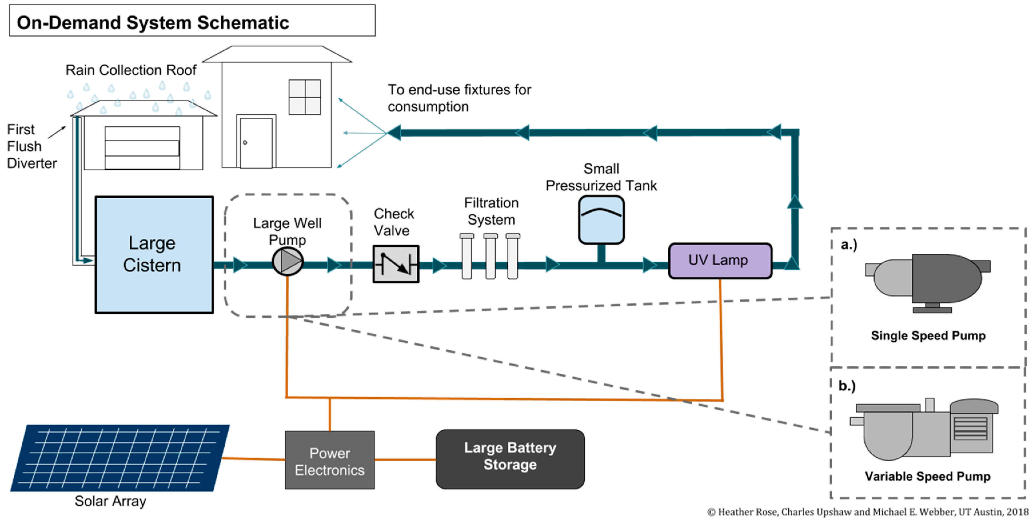
In these systems, water is collected off the catchment surface, and passes through one or more debris screens and a ‘first-flush diverter’ on its way to the primary storage tank. The primary storage is a large cistern that holds untreated harvested rainwater for eventual use. When a fixture in the home is in operation, water is pumped from the cistern through a filtration system, through a small pressure tank, through the inline UV treatment system, and finally to fixture delivery. The notional system is powered by electricity directly from solar photovoltaic (PV) panels when it is sunny enough to produce sufficient power, and from the battery during times of insufficient solar production. The battery is sized to provide the total amount of energy required by the pump and treatment system during non-solar producing hours (i.e., non-daylight and twilight hours). The pump is connected to a pressure switch that activates when the water pressure drops below a certain threshold, and the small pressure tank is used to keep the pump from short-cycling at low flow rates (i.e., the pump still starts for almost every water usage event). See Figure 1 below:
The On-Demand Systems Design consists of standard collection and treatment systems [2], with a pump (variable or single speed) that is powered by a PV and battery system, and a pressure control switch to activate it when water is used in the house.
2.2.2. Pressurized Water Storage (PS) Systems
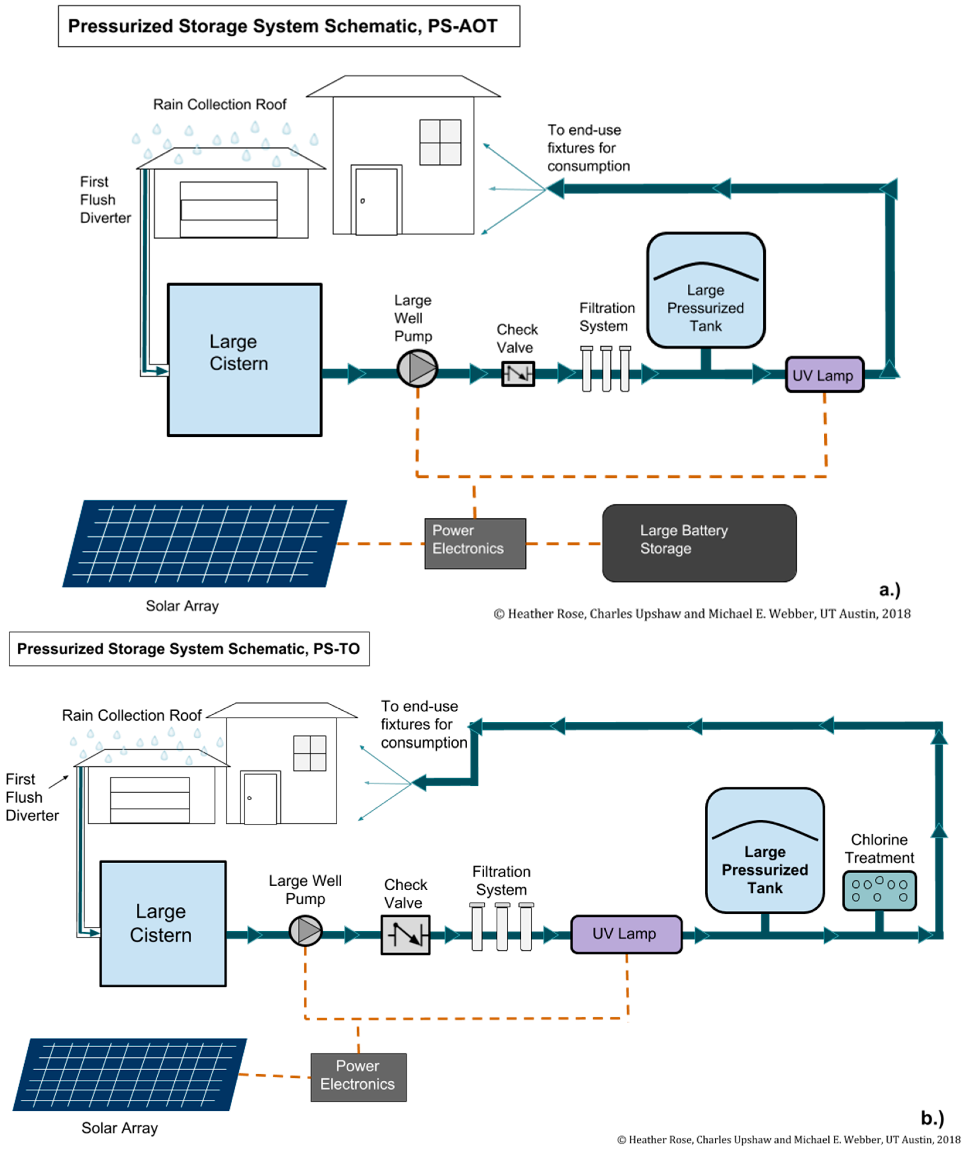
For the PS systems, we considered two scenarios: (1) treating water on-demand, and (2) treating water once per day. As in the On-Demand systems described above, water collected off the catchment surface passes through a ‘first-flush diverter’ then is stored in the cistern. During daylight hours, water is pumped via solar power from the cistern through a series of filters and into a large pressurized tank. For System A, a UV light is attached (powered by a battery) to the disposal end of the pressurized tank so water is treated on-demand with the UV light always on (PS-AOT). For System B, the UV light is only on while water is being pumped during the day (or treated once), using solar energy (PS-TO). The UV light can be powered by PV during times of sufficient PV production, just like the pumps. The System B configuration might be one where UV is used in conjunction with a chlorine dosing system such that water is dosed with sufficient treatment so that any residual water is sterilized. See Figure 2a,b below.
Our goal in comparing the PS-AOT system with the PS-TO system was to observe the impaction on capacity and size of the system when the UV lamp is only in operation once per day. Because of this, we anticipated seeing great energy savings in the PS-TO system, which is discussed later in the results section.
2.3. Residential Water Use Data Analysis
For our analysis, we used data from The Residential End Uses of Water in 2016 (REU2016 for short), which featured flow trace water meter data from 762 homes across the continental US [7]. For each home, a data point was taken every 10 s for two consecutive weeks [7]. A data set was then compiled featuring the anonymous house code, time stamp, event, duration, peak and average volume, for each water event, for two weeks. For our analysis, we reduced this original data set to only indoor events (toilets, showers, bathtubs, faucets, dishwashers and clothes washers) using Python. We found that when considering outdoor events, water consumption could exceed thousands of gallons per day. As such, we felt it would be more representative of typical water usage to only consider indoor events (see Supplemental Material for more information on Python Code). We further reduced the data set in Microsoft Excel with the Filter Tool by removing obvious outlier data (i.e., toilet events exceeding 100 gallons, or faucet events with durations longer than 60 min). To identify an appropriate volume range for events, we used the Home Water Works data as a reference to set our parameters for identifying outlier data points [10].
With this reduced data set, the mean average volume, duration and event count per hour were found. The average volume and duration per hour were used to calculate an average flow rate per hour to apply to a hydraulic pump power equation [11]. Using the event count average (, the frequency a pump was operated could be calculated to estimate pump startup energy. To find the average total daily volume, the average volume of water per hour was added for all hours, finding a total daily volume of 146 gallons (see Table A1 in Appendix A for these calculations).
It should be noted that all of the homes in the REU 2016 dataset were using municipally supplied water [7]. Therefore, it is possible that consumers were less conscientious about their water use since they did not have to store, treat, and pressurize their own water. Thus, consumption from this study is likely higher than a study with consumers who rely on an inherently limited water supply, for example from a backyard well. Therefore, the REU 2016 profile serves as a useful, conservative estimate for consumption in this initial analysis.
3. Modeling
3.1. On-Demand Systems Energy Modeling
For On-Demand systems, we considered two cases, one featuring a single-speed pump (OD-SS) that uses a constant steady state power rating regardless of the flow rate, and one featuring a variable-speed pump (OD-VS) that can alter power consumption based on flow rate. For the single-speed pump system, we gathered empirical data from a Grundfos MQ3-35B well pump (typically used in RWH systems [2]) (Downers Grove, IL, USA) to model startup and steady state power.
3.1.1. Empirical On-Demand Model (OD-SS)
For this model, we used the Grundfos pump empirical data that we gathered by turning on a MQ3-35B well pump five consecutive times while measuring the voltage and current required to turn the pump on and to reach steady state (see Table A2 for raw data). We considered the steady state power of the pump to be the steady state current of 2.6 A (seen in all five trials) multiplied by the measured voltage (213.7 V). This model approximates using a single-speed pump, which runs at full power when on, regardless of the actual flow rate demand. This setup is most common [2], as variable speed/constant supply pressure pumps are generally more expensive or are not as readily available as single speed pumps for small-scale residential water systems.
To calculate the startup energy, we summed the products of the current, voltage and time duration approaching the steady state current for all five trials, as shown in Equation (1), or:
The Pump Startup Energy was then taken to be the mean average startup energy of all five trials, or 0.0024 kWh (see Table A2 in Appendix A for more information on data and calculations).
To calculate the startup energy for each hour, we multiplied the average start up energy by the event count average (of number of times the pump was turned on) determined by the REU2016 data [7], or:
Using our empirical data from the Grundfos pump, we considered Pump Steady State Power to be simply the steady state current multiplied by the voltage, as shown in Equation (3), or:
To find the hourly energy, we multiplied the Pump Steady State Power by the average duration (or duration the pump was in use), summed with the pump startup energy multiplied by the event count average, and finally added to the UV lamp energy (run on battery power), as shown in Equations (4) and (5) below. The parameters for Equations (4) and (5) are defined in Table 1, along with their values and units. The nighttime energy use was divided by the battery round-trip efficiency because the system would be running on a battery, and incurring the energy penalty of the charge/discharge conversion. A battery round-trip efficiency ( of 0.89 was chosen based on the Tesla Powerwall 2 (Palo Alto, CA, USA) [12]:
To calculate total daily energy, we simply summed the calculated energies per hour for each hour from 1:00 a.m. to midnight, using Equation (4) for daylight hours and Equation (5) for nighttime hours.
Daylight hours were considered to be 8:00 a.m. to 4:00 p.m., or the number of daylight hours on Winter Solstice in Texas [13] subtracting two hours (the hour after sunrise and the hour before sunset) and considering those to be nighttime hours instead. These hours preclude PV generation due to the limited amount of incident radiation.
With these parameters and equations, we found the total daily energy for the OD-SS system to be 2.63 kWh (see Table A3 in Appendix A for the Calculation Table.)
3.1.2. Variable-Speed Pump Model (OD-VS)
For this system, we considered a variable-speed pump with the ability to alter power consumption based on flow rates. This variable-speed pump model is a simplified first-principles and theoretical model, which doesn’t account for real-world factors such as pump oversizing, or constant power consumption despite flow rate. With this, we expected energy requirements to be significantly lower than the empirical model. However, we saw merit in observing energy requirements solely based on the water consumption by the hour.
To calculate the steady state pumping power for each hour ‘i’ ( for the OD-VS system, we used the hydraulic pumping power relationship, shown in Equation (6) [11], with the flow-dependent total system head ( defined in Equation (7) [14] The total system head combines the static and flow-dependent frictional pressure by using the variable k, to account for frictional pressure drop due to pipes, fittings and fixtures in the flow path [14]:
where:
for which the variables for this equation are explained in Table 2.
To model the dynamic pressure drop, we followed the friction factor model of the square of the flow rate times the friction head loss coefficient, or [14]. To calculate the friction head loss coefficient C, we used a rated dynamic pressure drop of 25 m, or , and a rated flow rate of 5 gpm, or . Solving for C using these parameters, we found . This pressure head approximates pumping water through a treatment system below the house’s finish grade up to the various fixtures at a sufficient pressure.
To estimate the efficiency of a variable speed pump, we referred to the Aquatec 550 Series Aquajet Variable Speed Pump 12VDC 5 GPM (gallons per minute) manufacturer data [15]. We felt this pump model would adequately represent a variable speed pump that could handle a whole-home demand, if the users were to have multiple fixtures consuming water at the same time. For example, running a shower, a low-flow toilet, and faucet all running at once, their combined flow rates would be less than five gallons per minute (19 L per minute) [10].
From the Residential End Uses of Water 2016 study data, we found the average flow rate throughout the day was 1.5 gallons per minute (5.7 L per minute) [7]. Using the Aquatec 550 VS Pump 12VDC 5GPM manufacturer data, we found the power required to run this pump at a 1.5 gpm flow rate was 120 Watts [15]. To solve for pump efficiency, we rearranged the hydraulic pumping power relationship [11], as seen below in Equation (8). The parameters for Equation (8) are defined in Table 3, along with their values and units.
With these parameters, we found the pump efficiency for an average flow rate would be 27% for a variable speed pump.
To calculate the total energy consumed per hour, we used the results from Equation (6) and multiplied this by the average duration of use, while adding the energy for UV lamp. For nighttime hours (4:00 p.m. to 8:00 a.m.), this energy was divided by the battery round-trip efficiency, as discussed above. With this, we calculated the hourly energy consumption to be:
The parameters for Equations (9) and (10) are defined in Table 4 below, along with their values and units.
To calculate average total daily energy, we summed the calculated energy consumption per hour for each hour from 1:00 a.m. to midnight, using Equation (9) for daylight hours (8:00 a.m. through 4:00 p.m.) and Equation (10) for nighttime hours (between 5:00 p.m. and 7:00 a.m.). With these parameters and equations, we found the total daily power requirements for an OD-VS system was 1.65 kWh per day, for a total daily volume of 146 gallons (553 L) (see Table A4 in Appendix A for Calculation Table.)
3.2. Pressurized Storage Power and Energy Modeling
For the Pressurized Storage Systems, we assumed that water would be pumped into the large pressurized tank once a day, during daylight hours, using solar energy. Because water is being pumped once a day, we considered the Pump Startup Energy to be negligible and did not include it in this model. We also assumed that the large pressurized tank would provide sufficient pressure and no additional pumps would be needed for fixture delivery.
For this system type, we considered pump energy requirements for pumping a day’s supply of water (146 gallons, or 553 L) within different refill durations (45 min, 1 h and 4 h) using three different sized pumps. The flow rate for this model was defined as the total volume of water (0.55 m3) divided by the refill duration (Δ
3.2.1. UV Treatment on Demand with UV Lamp Always on (PS-AOT)
For this system, we considered the UV Lamp to be always on, 24 h a day, using battery power at night. In this system, the UV Lamp is connected to the disposal end of the large pressurized tank for on-demand treatment of water when moving to a fixture. See Figure 2a above.
To model the pump efficiency we again used Equation (8), along with the power draw, pressure head and flow rate manufacturer data from Seaflo 12V Diaphragm single speed pumps (Freehold, NJ, USA) [16,17]. The Seaflo 21 Series 12V DC Diaphragm Pump 1.1 GPM Capacity was used to model a small pump with a low flow rate [16]. The Seaflo 52 Series 12V DC Diaphragm Pump 4 GPM Capacity [17] was used to model a medium sized pump with a moderate flow rate. The Seaflo 52 Series 12V DC Diaphragm Pump 5 GPM Capacity [17] was used to model a large pump with a high flow rate. With the manufacturer data from the Seaflo 21 and 52 series pumps, we solved for using Equation (11) below. The parameters for Equation (11) are defined in Table 5, along with their values and units.
with the following parameters:
With Equation (11) and the above parameters, we calculated a pump efficiency value for a small sized pump to be 38%, a medium sized pump to be 42% and a large sized pump to be 43%.
To calculate the Pump Steady State Power, we used a similar equation to that of Equation (6), but with an assigned time interval for flow rate. The assigned time intervals coincided with an assigned pump efficiency to match an appropriate flow rate with an appropriately sized pump. Specifically the 45 min pump time coincided with for a high flow rate, the 1 h pump time coincided with for a moderate flow rate, and the 4 h pump time coincided with for a low flow rate.
To model static and dynamic pressure drop, we again used a constant value for the static pressure summed with the dynamic pressure drop based on flow rate [14]. We increased the static pressure drop to 30 m (42.6 PSI) to account for the loss of pressure in the tank during use. It was assumed the pressure tank would be operating in the range of 30–50 PSI, a typical range for pressure tanks [2]. The pump re-pressurizing the system would be working against a higher static pressure. The higher pressure in the storage tank is necessary to provide sufficient pressure to overcome both static and frictional pressure losses when the tank is nearly empty.
For the dynamic pressure drop k, we again set the friction head loss coefficient C to be and multiplied this by the flow rate squared.
Using these pump efficiencies, we were able to calculate the pump power for the three assigned pump times using Equation (12) below. The parameters for Equation (12) are defined in Table 6 below, along with their values and units.
with the following parameters:
Using Equation (12) with the parameters indicated above, we found the pump power requirement for the PS-AOT system ranged from 0.03 to 0.19 kW based on the flow rate and pump size. See Table A5 in Appendix A for Calculations.
Total daily energy, (shown in Equation (13)) was then calculated by multiplying the pump steady state power ( by the assigned time interval ( adding the power for the UV lamp ( multiplied by daytime hours, plus the power for the UV lamp ( multiplied by nighttime hours, accounting for battery round-trip efficiency (. Table 7 below defines these variables and the values used for this analysis:
With these parameters and equations, we found the total daily energy required for the PS-AOT system to range from 1.67 kWh for the small pump to 1.69 kWh for the large pump, or the average daily energy for PS-AOT system was 1.68 kWh for small, medium and large pumps (see Table A5 in Appendix A for Calculation Table).
3.2.2. UV Treatment Once per Day (PS-TO)
In the PS-TO system, water is treated prior to entering the large pressurized tank for storage. The UV lamp is then only on during the assigned time interval for pumping the water. See Figure 2b above.
For the PS-TO pump steady state power, we also used the results from Equation (13). However, for the total daily energy, we reduced the UV lamp energy factor to be powered only during the assigned pump time, as shown in Equation (14) below. The parameters for Equation (14) are defined in Table 8 below, along with their values and units.
With these parameters and equations, we found that total energy requirements varied by assigned pump time and pump size from 0.19 kWh per day to 0.36 kWh per day. See Table 9 below:
3.3. Cost Comparison between Systems
For a normalized estimated cost equation to compare between systems, we considered a price average per capacity for batteries, PV arrays, pumps, UV lamps and pressurized tanks. We gathered prices for battery bank and PV array kits from an online solar equipment wholesaler to use as representative cost estimates for these system components [18]. Similarly, prices for single speed, constant pressure (variable speed) pumps, and UV lamps were gathered from an online rainwater harvesting equipment seller [19]. We normalized the prices by dividing the component cost by its capacity to obtain a Price-to-Capacity (PC) scaling factor for estimating system costs, as per Equation (15) below. In this analysis, the battery banks were scaled per kWh of capacity, the PV arrays by unit of average winter day kWh production, the pumps were scaled by rated maximum watts of power demand, UV lamps were scaled per GPM capacity, and the pressurized tanks were scaled by drawdown capacity. We took the average of these PC ratios for a variety of equipment to obtain a representative average estimate. Equation (15) below describes the PC factor for Battery Banks, PV arrays, Single Speed, Constant pressure pumps, UV Lamps and pressurized tanks:
When choosing batteries to include in Equation (15a), we only considered batteries with a minimum storage capacity of 2 kWh. We gathered prices for different lithium-ion batteries from the Wholesale Solar website [18] and used Equation (15a) to calculate a Price-to-Capacity scaling factor. See Table A6 in Appendix A for calculation.
When choosing PV panels to include in Equation (15b), we only considered solar panels with a minimum power capacity of 1 kW. Using the PVWatt Calculator developed by N.R.E.L. (Golden, CO, USA) [20], we determined that a 1 kW solar panel could successfully generate 3.03 kWh per day in December in Austin, TX, USA, which exceeds the maximum energy requirements for all four systems. We gathered prices for different PV panels at a minimum of 1 kW capacity from the Wholesale Solar website and used Equation (15b) to calculate a Price-to-Capacity scaling factor. See Table A7 in Appendix A for calculation.
When choosing pumps and UV lamps to include in Equations (15c)–(15e), we ensured that all items had the minimum flow rate capacity to handle their respective system demands. We gathered prices for different pumps (both single speed and variable speed) and UV lamps from the Rainwater Harvesting Supplies website [19] and used Equations (15c)–(15e) to calculate the Price-to-Capacity scaling factors. See Table A8 and Table A9 in Appendix A for , and calculations.
For the PS systems, we found pressure tanks that were in the range of over 80 gallons of drawdown capacity [21,22], as the daily water volume requirement was 146 gallons for each home. The list price of the tank was multiplied by the number of tanks that would need to be purchased to store 146 gallons of pressurized water with the tanks in series. We then divided the total price of the tanks by the total capacity to calculate the Price to Capacity scaling factor for pressurized tanks. This PC factor was multiplied by the required volume of 146 gallons to get a dollar amount for the pressurized tanks. See Table A10 in Appendix A for calculations.
We found that prices for system components varied based on their respective capacities. We did, however, see a general trend of the greater the capacity, the lower the PC. Price, capacity and PC ranges can be seen in Table 10 below.
To obtain a total system cost estimate (), we multiplied the PC coefficients by the daily energy, peak pump power, and average flow rate values respectively to obtain a system value in dollars. We then multiplied these variables by an Oversize Factor () to account for days of unexpectedly high use. We added the product of the average flow rate with the PC coefficient for the UV lamp and the storage requirements with the PC coefficient for the pressurized tank.
The estimated cost of each system was calculated by:
The parameters for Equation (16) are defined in Table 11 below, along with their values and units.
Using Equation (16) along with the values, we obtained from the energy and power analysis for each system and pricing information for battery banks, PV arrays, pumps, UV lamps and large pressurized tanks, we were able to come up with a table of estimated maximum prices per system, the results of which are shown below in Table 12:
Using the OD-SS system as a base, as it is the most common system setup [2], we then normalized these estimated prices to calculate a percentage to compare prices between systems based on their respective energy requirements. Table 13 below summarizes the percent differences between the baseline system capital cost and the other systems.
4. Results and Discussion
4.1. System Energy Analysis
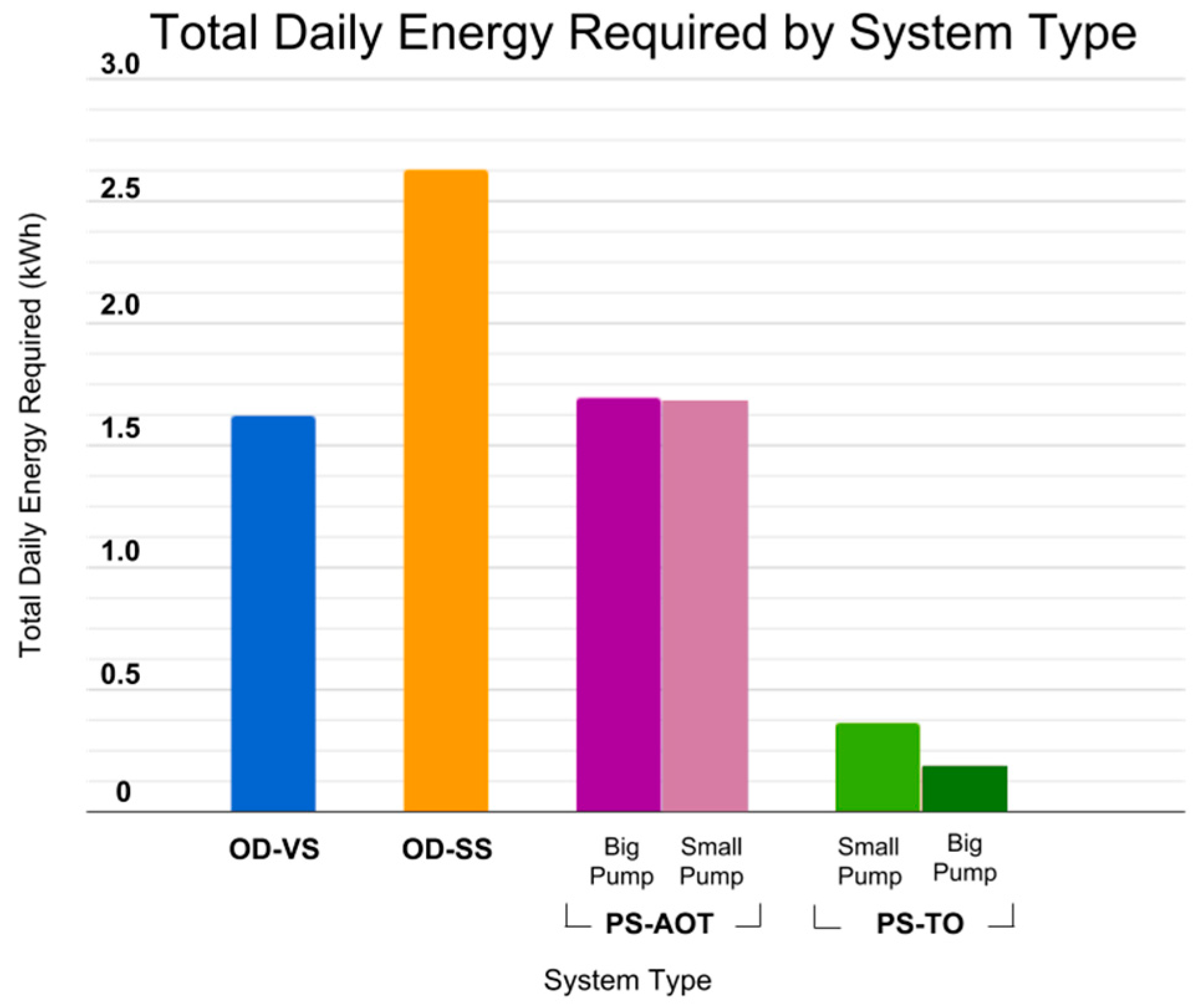
From our analysis, we found the OD-SS required the highest total daily energy requirement of 2.63 kWh/day. The OD-VS and the PS-AOT systems had similar maximum energy requirements of 1.65 and 1.69 kWh per day, respectively. The PS-TO system had the lowest daily energy requirements, ranging from 0.19 to 0.36 kWh per day based on assigned pumping time and pump size. See Figure 3 below.
4.1.1. Empirical On-Demand System (OD-SS)
For the OD-SS system, we found the total daily energy requirement was 2.63 kWh, which is 60% more than that of the OD-VS system. The maximum power needed for the OD-SS system was 0.62 kW when only considering steady state power (startup power demand can spike 10–25% higher). We think these values are much more representative of the actual energy requirements for an on-demand system as it models the real-world dilemma of pump over-sizing. When purchasing a pump, one must size for a maximum flow rate in order to prevent pump failure. However, pumps are designed to perform at maximum efficiency when operating at higher flow rates. As seen from the Residential End Uses of Water 2016 data [7], flow rates are relatively low compared to pump capacity. This over capacity of the pump results in more energy consumption because the excess pressurization is throttled at the tap (or other end-use), wasting much of the energy put into pressurizing the water.
4.1.2. Variable-Speed Pump On-Demand System (OD-VS)
We found the total daily energy requirement for the OD-VS system was 1.65 kWh per day, while the maximum power needed was 0.180 kW (when considering a peak flow rate of 4.5 GPM [15]). Our variable speed on-demand pump model was based on theoretical pump power equations, with flow rates averaged from the uses each hour, pressure drop simplified to a quadratic system curve, and efficiency coefficients made constant for simplification. This equation calculates the power needed to deliver water at the calculated flow rate and pressure drop, but it does not capture the potential inefficiencies of very low part-load operation nor the potential increase in power for delivering significantly higher volumes of water. These shortcomings in modeling pump performance have been identified by Ward in 2012 [6] and others, but this method is useful for providing a generalized order of magnitude estimate for the power demand and energy consumption for an on-demand variable speed system. Keeping these simplifications in mind, we still estimate that there could be significant energy savings by using a variable speed pump instead of a single speed pump for residential rainwater systems.
4.1.3. Pressurized Storage, UV On-Demand Treatment System (PS-AOT)
For the PS-AOT system, we found the daily energy required for small, medium, and large sized pumps ranged from 1.67 to 1.69 kWh. The main power consumer in this system is the UV lamp, requiring 1.55 kWh of energy per day. Conversely, the energy required for pumping was only 0.12–0.14 kWh per day. The pump power requirements for this system ranged from 0.03 to 0.19 kW depending on the designated flow rate and pump size. We can see in this system that while there are savings from operating a smaller pump for a longer period of time (thus reducing frictional pressure drop), these relative savings are dwarfed by the energy needs of the always-on treatment system. The relative differences between the larger, faster pump and the smaller, slower pump are system-dependent, and there could be no savings from the smaller pump if the system is static pressure dominated.
4.1.4. Pressurized Storage, UV Once a Day Treatment (PS-TO)
For the PS-TO system, we found that the total energy requirements varied by assigned treatment time and pump size (0.19–0.36 kWh for treatment times between 0.75 and 4 h). Interestingly, in this system configuration, the scenario with the small pump consumes the most energy because the longer fill duration means the UV lamp is on for hours longer, which swamps the lower pumping energy savings. We see significant energy savings for the largest pump size, despite higher pumping energy, due to the shorter time-period that the UV lamp is in operation. When comparing the PS-TO system to the PS-AOT, we see significant energy savings across the board due to only operating the UV lamp while pumping the water into the pressurized tank.
It should be noted that treating water before storing it comes with a risk of contamination. If the tank is not emptied completely on a regular basis, residual water that was treated days before could remain in the tank, allowing residual biologic contaminants to slowly build to a level that is no longer safe for consumption. This risk of contamination is why RWH systems typically position the UV treatment last in the assembly before delivery to a house plumbing [2]. It should also be noted that UV lamps have a “warm up time” before they reach full treatment capacity. Therefore, using this configuration on its own, without a means to properly periodically flush the pressure tank, and/or without a secondary residual treatment system (e.g., chlorine or ozone), should be limited to applications where non-potable water is suitable.
4.1.5. Power and Energy Storage Requirements between Systems
Comparing these four system configurations, we can see a significant difference in PV capacity and battery storage requirements between systems. The OD-SS system has a maximum power requirement of 0.62 kW and to run this system at night requires a minimum battery storage of 1.65 kWh per day. In comparison, the OD-VS system requires a maximum power of 0.18 kW and to run this system at night requires a minimum of 1.07 kWh of battery storage.
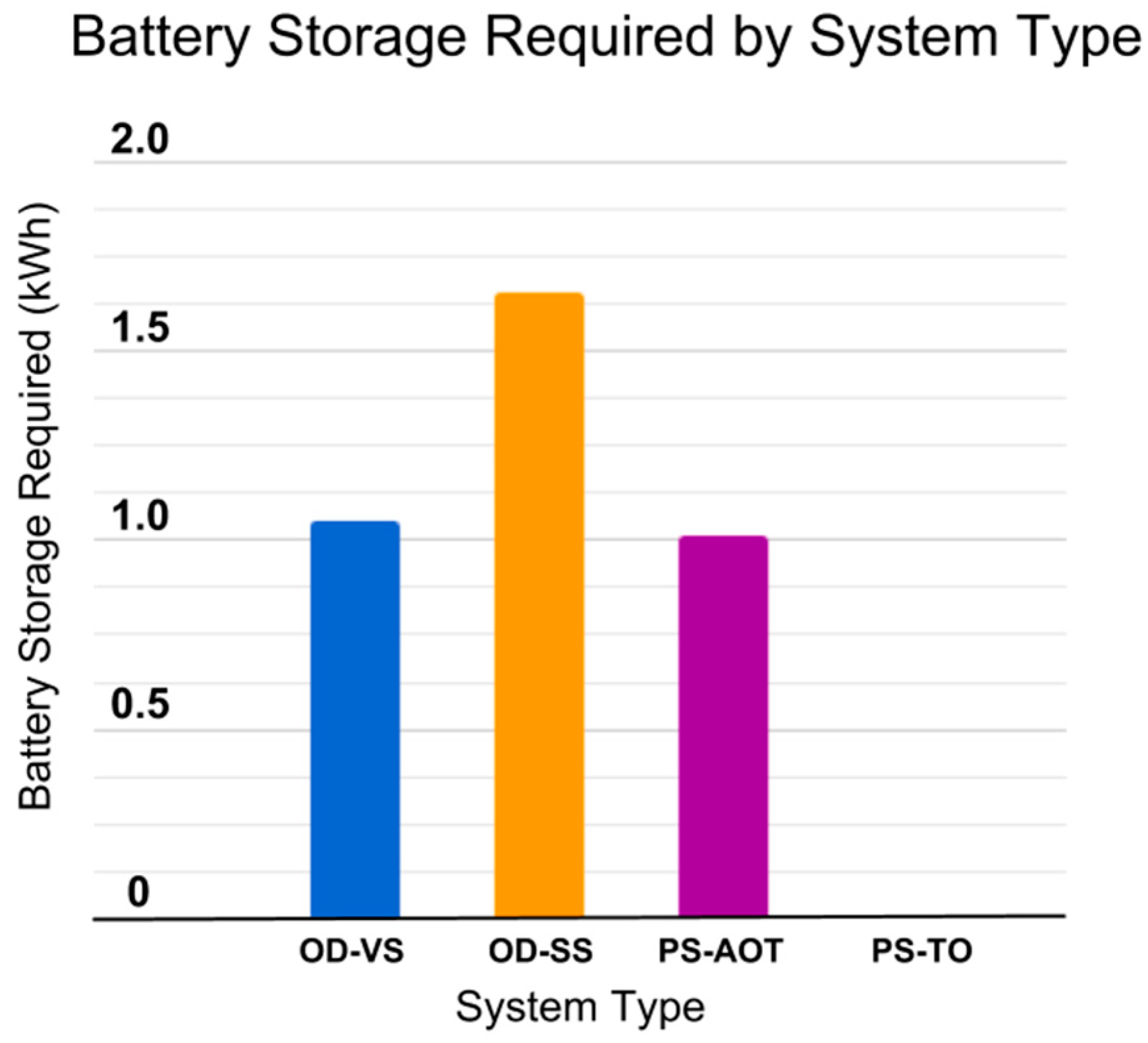
By comparison, the PS-AOT and the PS-TO models both have a maximum power requirement of 0.25 kW. The PS-AOT system requires a battery storage of 1.01 kWh per day to power the UV lamp at night, whereas the PS-TO system does not require any additional battery storage as both pumping and treatment occur during daylight hours using solar energy. See Figure 4 and Figure 5 below for a comparison of required Power and Battery Storage between systems.
Overall, these results show that the battery storage requirements for the OD-SS system is the highest due to the combined energy needed to run an over-sized pump and treat water on demand. The OD-VS and PS-AOT systems’ battery storage requirements are relatively similar due to the UV lamp energy being the main driver for energy consumption in both scenarios.
4.2. System Cost Analysis
From our analysis, the OD-SS system is the most expensive. We believe that this is due to the extra energy requirements of a single speed, oversized pump that operates at a higher energy capacity than necessary. We can see the OD-VS and the PS-AOT systems are similar in price range, despite having different system configurations. The PS-AOT system requires pressurized tanks, in the 100+ gallon capacity range, mostly accounting for the difference in price between the OD-VS and the PS-AOT systems.
From our analysis, the least expensive system is the PS-TO system. This system saves a lot of energy because water is only pumped and treated once per day, removing the necessity for battery storage all together. In addition, because water is pumped once per day, at a designated flow rate, a single speed appropriately sized pump can be used, significantly reducing costs.
Comparing these systems via our analysis, we can see the biggest driver for cost is the amount of PV energy and battery storage required for each system. In fact, battery storage alone makes up for 39% of the OD-SS system’s cost requirements, 42% of the OD-VS system’s cost requirements, and 30% of the PS-AOT system’s cost requirements. The extra cost of the large pressurized tank for the PS systems seemed to affect total cost the least. This being said, systems with lower energy demand can significantly reduce costs by reducing the need for large PV arrays and battery storage.
The best value system, by far, is the PS-TO system, because of its very low energy requirements. Because this system has a set flow rate chosen by the operator, a significantly smaller (and less expensive) single speed pump can be used. In addition, the PV array can be sized appropriately (only providing power for items actively in use), which significantly reduces cost.
Although the PS-TO system is the most energy and cost effective of the four systems, there is always a risk of contamination with stored water as discussed above. For this reason, we recommend adding a secondary treatment directly before consumption (such as chlorine, reverse osmosis, etc.)
It should be noted that the above cost analyses only consider the prices based on energy, power and flow rate capacities. When pricing out a system, it is very unlikely that items such as battery banks, PV arrays and UV lamps will be available at the exact capacities described in this analysis. Due to market demand, additional costs should be anticipated for battery banks, PV arrays and UV lamps at higher than necessary capacities. However, the purpose of this analysis was not to provide comprehensive system cost estimates, but rather to analyze the relative differences in cost between these system configurations to get an understanding of the underlying driving factors.
Additionally, it also should be noted that this analysis only considers upfront capital costs. Further analysis would need to be conducted to investigate the additional operational and maintenance costs of replacing pumps, batteries, PV arrays and tanks as they degrade over time. This analysis does not consider the long-term loss in energy efficiency due to battery life cycles and solar panel degradation. The more the battery and solar panel are used, the less life cycles remain, contributing to loss in efficiency. Further analysis would need to be conducted to see how great of a contributor this loss in efficiency would be.
This analysis only considers costs for the energy consuming components of a rainwater harvesting system for the purpose of comparing costs between system types. Further analysis would need to be conducted to estimate costs of cisterns, filters, pipes, etc. that are also required components of any complete rainwater harvesting system [2].
For safety, we recommend having the ability to create an On-Demand treatment and delivery system in case more water is consumed than was treated and stored. In addition, homes should always have access to municipal water supply in case of malfunction, water contamination or water shortages.
5. Conclusions and Future Work
The purpose of this paper was to model the energy requirements of four different configurations for rainwater harvesting systems and to compare these systems by total energy requirements and relative costs. We aimed to answer the question: Can energy be saved by utlizing variable speed pumps or pressurized storage tanks? In addition—Does altering the system configuration lower the overall cost of the system?
We found that the most traditional configuration of the OD-SS system was in fact the most energy intensive and most expensive system setup. Our analysis showed that this is due to oversizing the pump and to powering a UV lamp 24 h a day. We found that energy and money could be saved by using a variable speed pump for on-demand systems, or by storing a day’s worth of water and replacing an on-demand pump with a large pressurized tank. Our analysis also showed that the UV lamp’s energy consumption was non-trivial, and only turning it on when in use significantly lowered the energy requirements of the system. From our cost analysis, we found the most expensive components of the system to be the PV array size and battery storage requirements to meet the system’s energy needs. We found the most energy efficient and least expensive setup to be the PS-TO system, due to its very low energy demand.
As with any model, it is always best legitimized by predicting results from empirical data. For this project, obtaining relevant power and energy data for a potable residential RWH system was challenging. For our future work, we plan to monitor an active RWH system to gather empirical data on the power requirements to pump, treat, and deliver water based on the system configurations discussed in this paper. With this data, we will be able to directly compare our model to see where adjustments need to be made.
An important consideration for any type of water storage is the quality of the water after it has been stored for a period of time. Upon building a small-scale PS system, we plan to test the quality of the water exiting the system over a long-term test (6–12 months) to evaluate how the system water quality might change over time.
The less water consumed, the more potential energy savings from lowering the demand for pumping and treating water. Incorporating grey water usage for toilets and clothes-washers could potentially dramatically lower the power requirements of the system due to working with lower volumes. In future analysis, we plan to include grey-water use in the model by eliminating toilet and clothes-washer events.
This study will soon feature an online visualizer to show water consumption by hour for all homes in the Residential End Uses of Water study of 2016. It will feature filters to view data based on end use (toilet, shower, irrigation, etc.), region of the country, month of the year, and weekday vs. weekend water consumption. This module is being developed in Python using a Bokeh visualizer.
This study will also feature an online calculator to assist with sizing custom systems. It will contain inputs for anticipated volume of daily water consumption, water use schedules, pressure head, UV lamp wattage and more. Once a system size has been selected, the module will guide you through how large of a pump, solar array, and battery you will need to run the system. The calculator will also include power and water savings by incorporating grey water use for toilets, clothes washers and irrigation.
Supplementary Materials
Python code and extended information of data used for this paper can be found on the author’s website: https://heatherscarlettrose.com/research/REU2016-python-code; https://heatherscarlettrose.com/research/REU2016-data-tables.
Author Contributions
The original motivation and driving hypotheses for this analysis was developed by C.U. H.R. carried out the bulk of the analysis and writing, working closely with C.U. on the modeling and interpretation of the results. M.W. oversaw the research, and provided feedback and quality control.
Funding
This research was funded in part by the University of Texas at Austin Green Fee Student Research Grant program, Pecan Street, Inc., the Texas Emerging Technology Fund (OSP 201404029001), and the Cynthia and George Mitchell Foundation. A full list of sponsors for all projects in Webber’s research group at UT are listed at http://www.webberenergygroup.com/about/sponsors. Webber’s affiliations and board positions are listed at http://www.webberenergygroup.com/people/michael-webber.
Acknowledgments
The authors would like to thank the Engineering Scientist Juan Diego Rodriguez for assistance with Python and Bokeh code.
Conflicts of Interest
In addition to research work on topics generally related to energy systems at the University of Texas at Austin, Charles Upshaw and Michael Webber are equity partners in IdeaSmiths LLC (Austin, TX, USA), which consults on topics in the same areas of interest. The terms of this arrangement have been reviewed and approved by the University of Texas at Austin in accordance with its policy on objectivity in research.
Appendix A. Data and Calculation Tables

Table A1.
Analyzed data from the Residential End Uses of Water 2016 study.
| Hour | Mean Water Vol (m3) | Mean Duration (s) | Event Count Avg. | |
|---|---|---|---|---|
| 0 | 3 | 0.011 | 193 | 1 |
| 1 | 3 | 0.011 | 114 | 1 |
| 2 | 2 | 0.008 | 93 | 0 |
| 3 | 2 | 0.008 | 95 | 0 |
| 4 | 3 | 0.011 | 127 | 1 |
| 5 | 5 | 0.019 | 202 | 1 |
| 6 | 8 | 0.030 | 298 | 2 |
| 7 | 9 | 0.034 | 347 | 3 |
| 8 | 9 | 0.034 | 333 | 3 |
| 9 | 9 | 0.034 | 331 | 3 |
| 10 | 8 | 0.030 | 313 | 2 |
| 11 | 7 | 0.026 | 282 | 2 |
| 12 | 7 | 0.026 | 273 | 2 |
| 13 | 7 | 0.026 | 261 | 2 |
| 14 | 6 | 0.023 | 246 | 2 |
| 15 | 6 | 0.023 | 244 | 2 |
| 16 | 6 | 0.023 | 251 | 2 |
| 17 | 7 | 0.026 | 278 | 3 |
| 18 | 7 | 0.026 | 286 | 3 |
| 19 | 7 | 0.026 | 294 | 3 |
| 20 | 7 | 0.026 | 275 | 2 |
| 21 | 7 | 0.026 | 256 | 2 |
| 22 | 6 | 0.023 | 221 | 2 |
| 23 | 5 | 0.019 | 170 | 1 |
| Total Daily Volume: 146 gal, 0.55 m3 | ||||
| Avg. Daily Flow Rate (m3/s): | 0.000094 | |||
| Avg. Daily Flow Rate (gal/min): | 1.50 | |||
| Max Daily Flow Rate (m3/s) | 0.000111 | |||
| Min Daily Flow Rate (m3/s) | 0.000059 | |||
| Max Daily Flow Rate (gal/min): | 1.76 | |||
| Min Daily Flow Rate (gal/min): | 0.93 | |||
Table A2.
Grundfos Pump Startup Energy, Collected Data.
| Trial A Time (s) | Current (A) | Voltage (V) | Power (W) | Energy (kWs) | Startup Energy (kWh) |
| 0 | 0 | 213.7 | 0 | 0.00224 | |
| 1 | 5.6 | 213.7 | 1196.72 | 1.20 | |
| 3 | 2.8 | 213.7 | 598.36 | 1.20 | |
| 6 | 2.8 | 213.7 | 598.36 | 1.80 | |
| 13 | 2.6 | 213.7 | 555.62 | 3.89 | |
| Trial B Time (s) | Current (A) | Voltage (V) | Power (W) | Energy (kWs) | Startup Energy (kWh) |
| 0 | 0 | 213.7 | 0 | 0.00213 | |
| 1 | 3.3 | 213.7 | 705.21 | 0.71 | |
| 3 | 2.8 | 213.7 | 598.36 | 1.20 | |
| 8 | 2.8 | 213.7 | 598.36 | 2.99 | |
| 9 | 2.6 | 213.7 | 555.62 | 0.56 | |
| 13 | 2.6 | 213.7 | 555.62 | 2.22 | |
| Trial C Time (s) | Current (A) | Voltage (V) | Power (W) | Energy (kWs) | Startup Energy (kWh) |
| 0 | 0 | 213.7 | 0 | 0.00203 | |
| 1 | 4.4 | 213.7 | 940.28 | 0.94 | |
| 3 | 2.8 | 213.7 | 598.36 | 1.20 | |
| 5 | 2.8 | 213.7 | 598.36 | 1.20 | |
| 9 | 2.7 | 213.7 | 576.99 | 2.31 | |
| 12 | 2.6 | 213.7 | 555.62 | 1.67 | |
| Trial D Time (s) | Current (A) | Voltage (V) | Power (W) | Energy (kWs) | Startup Energy (kWh) |
| 0 | 0 | 213.7 | 0 | 0.00342 | |
| 1 | 5.3 | 213.7 | 1132.61 | 1.13 | |
| 2 | 2.8 | 213.7 | 598.36 | 0.60 | |
| 5 | 2.8 | 213.7 | 598.36 | 1.79 | |
| 8 | 2.8 | 213.7 | 598.36 | 1.79 | |
| 10 | 2.8 | 213.7 | 598.36 | 1.2 | |
| 14 | 2.8 | 213.7 | 598.36 | 2.39 | |
| 17 | 2.7 | 213.7 | 576.99 | 1.73 | |
| 20 | 2.6 | 213.7 | 555.62 | 1.67 | |
| Trial E Time (s) | Current (A) | Voltage (V) | Power (W) | Energy (kWs) | Startup Energy (kWh) |
| 0 | 0 | 213.7 | 0 | 0.00240 | |
| 2 | 4 | 213.7 | 854.80 | 1.71 | |
| 3 | 2.8 | 213.7 | 598.36 | 0.60 | |
| 6 | 2.8 | 213.7 | 598.36 | 1.79 | |
| 8 | 2.7 | 213.7 | 576.99 | 1.15 | |
| 10 | 2.7 | 213.7 | 576.99 | 1.15 | |
| 14 | 2.6 | 213.7 | 555.62 | 2.22 | |
| Grundfos Pump Startup Energies. | Value | ||||
| Trial A (kWh) | 0.00224 | ||||
| Trial B (kWh) | 0.00213 | ||||
| Trial C (kWh | 0.00203 | ||||
| Trial D (kWh) | 0.00342 | ||||
| Trial E (kWh) | 0.00240 | ||||
| Avg. Startup Energy (kWh) | 0.00244 | ||||
Table A3.
Empirical on-demand system calculations.
| Parameter | Value | ||||
| Pump Startup Energy (kWh) | 0.00244 | ||||
| (kW) | 0.06 | ||||
| 0.89 | |||||
| Hour | Mean Duration (s) | Event Count Avg. | Pump Power (kW) | Pump Startup Energy (kWh) | Energy per Hour (kWh) |
| 0 | 193 | 1 | 0.56 | 0.00244 | 0.104 |
| 1 | 114 | 1 | 0.56 | 0.00244 | 0.090 |
| 2 | 93 | 0 | 0.56 | 0.00000 | 0.084 |
| 3 | 95 | 0 | 0.56 | 0.00000 | 0.084 |
| 4 | 127 | 1 | 0.56 | 0.00244 | 0.092 |
| 5 | 202 | 1 | 0.56 | 0.00244 | 0.105 |
| 6 | 298 | 2 | 0.56 | 0.00489 | 0.125 |
| 7 | 347 | 3 | 0.56 | 0.00733 | 0.136 |
| 8 | 333 | 3 | 0.56 | 0.00733 | 0.119 |
| 9 | 331 | 3 | 0.56 | 0.00733 | 0.119 |
| 10 | 313 | 2 | 0.56 | 0.00489 | 0.114 |
| 11 | 282 | 2 | 0.56 | 0.00489 | 0.109 |
| 12 | 273 | 2 | 0.56 | 0.00489 | 0.107 |
| 13 | 261 | 2 | 0.56 | 0.00489 | 0.105 |
| 14 | 246 | 2 | 0.56 | 0.00489 | 0.103 |
| 15 | 244 | 2 | 0.56 | 0.00489 | 0.103 |
| 16 | 251 | 2 | 0.56 | 0.00489 | 0.104 |
| 17 | 278 | 3 | 0.56 | 0.00733 | 0.124 |
| 18 | 286 | 3 | 0.56 | 0.00733 | 0.126 |
| 19 | 294 | 3 | 0.56 | 0.00733 | 0.127 |
| 20 | 275 | 2 | 0.56 | 0.00489 | 0.121 |
| 21 | 256 | 2 | 0.56 | 0.00489 | 0.118 |
| 22 | 221 | 2 | 0.56 | 0.00489 | 0.112 |
| 23 | 170 | 1 | 0.56 | 0.00244 | 0.100 |
| Total Daily Energy: | 2.63 kWh | ||||
| 4.76 | |||||
Table A4.
Variable-speed pump on demand system calculations.
| Parameter | Value | ||||
| 15 | |||||
| 2.51 × 10⁸ | |||||
| 1000 | |||||
| 9.81 | |||||
| 0.27 | |||||
| (kW) | 0.06 | ||||
| 0.89 | |||||
| Hour | Mean Duration (s) | K_friction | Pump Power (kW) | Energy per Hour (kWh) | |
| 0 | 0.000059 | 193 | 1 | 0.034 | 0.069 |
| 1 | 0.000100 | 114 | 2 | 0.063 | 0.070 |
| 2 | 0.000081 | 93 | 2 | 0.049 | 0.069 |
| 3 | 0.000080 | 95 | 2 | 0.048 | 0.069 |
| 4 | 0.000089 | 127 | 2 | 0.055 | 0.070 |
| 5 | 0.000094 | 202 | 2 | 0.059 | 0.071 |
| 6 | 0.000102 | 298 | 3 | 0.065 | 0.073 |
| 7 | 0.000098 | 347 | 2 | 0.062 | 0.074 |
| 8 | 0.000102 | 333 | 3 | 0.065 | 0.066 |
| 9 | 0.000103 | 331 | 3 | 0.066 | 0.066 |
| 10 | 0.000097 | 313 | 2 | 0.061 | 0.065 |
| 11 | 0.000094 | 282 | 2 | 0.059 | 0.065 |
| 12 | 0.000097 | 273 | 2 | 0.061 | 0.065 |
| 13 | 0.000102 | 261 | 3 | 0.065 | 0.065 |
| 14 | 0.000092 | 246 | 2 | 0.057 | 0.064 |
| 15 | 0.000093 | 244 | 2 | 0.058 | 0.064 |
| 16 | 0.000090 | 251 | 2 | 0.056 | 0.064 |
| 17 | 0.000095 | 278 | 2 | 0.060 | 0.073 |
| 18 | 0.000093 | 286 | 2 | 0.058 | 0.073 |
| 19 | 0.000090 | 294 | 2 | 0.056 | 0.073 |
| 20 | 0.000096 | 275 | 2 | 0.061 | 0.073 |
| 21 | 0.000104 | 256 | 3 | 0.066 | 0.073 |
| 22 | 0.000103 | 221 | 3 | 0.066 | 0.072 |
| 23 | 0.000111 | 170 | 3 | 0.073 | 0.071 |
| Total Daily Energy: | 1.65 kWh | ||||
| 2.99 | |||||
Table A5.
Pressurized storage, UV lamp always on calculations.
| Parameter | Value | ||||
| 30 | |||||
| 2.51 × 10⁸ | |||||
| Total Volume (m3) | 0.55 | ||||
| 1000 | |||||
| 9.81 | |||||
| (kW) | 0.06 | ||||
| 0.89 | |||||
| Pump Time (h) | Pump Size | Pump Efficiency | Pump Power (kW) | Total Daily Energy (kWh) | |
| 0.75 | Large | 0.43 | 0.00020 | 0.19 | 1.69 |
| 1 | Medium | 0.42 | 0.00015 | 0.13 | 1.68 |
| 4 | Small | 0.38 | 0.00004 | 0.03 | 1.67 |
Table A6.
Price per capacity scaling factor calculations for batteries.
| Lithium-Ion Battery | Price | Lifespan * | Capacity (kWh) | P/C $/kWh |
| Discover Battery 260AH 48VDC 13,200 Wh (2) Lithium Battery | $13,195 | 10 years | 12.5 | $1056 |
| Discover Battery 520AH 48VDC 26,400 Wh (4) Lithium Battery | $26,475 | 10 years | 25 | $1059 |
| Discover Battery 650AH 48VDC 33,000 Wh (5) Lithium Battery | $32,975 | 10 years | 31.2 | $1057 |
| Discover Battery 220AH 24VDC 5600 Wh (2) Lithium Battery | $6495 | 10 years | 5.3 | $1225 |
| P/C Avg LI Batteries: | $1099 | |||
| Information accessed from: | ||||
| www.wholesalesolar.com/solar-battery-banks | ||||
| (Accessed on 11 July 2018) |
* Lifespan based on warranty length.
Table A7.
Price per capacity scaling factor calculations for PV arrays.
| PV System | Price | Power Capacity kW | Energy Capacity kWh (Winter) | P/C $/kWh |
| Cabin 2.65 kW 9 Panel Solar World | $9559 | 2.65 | 5.97 | $1601 |
| Cabin 2.43 kW 9 Panel Candian Solar | $8795 | 2.43 | 5.47 | $1608 |
| Cabin 1.77 kW 6 Panel Solar World | $8379 | 1.77 | 3.98 | $2105 |
| Cabin 1.62 kW 6 Panel Canadian Solar | $7870 | 1.62 | 3.64 | $2162 |
| Cabin 1.18 kW 4 Panel Solar World | $6960 | 1.18 | 2.65 | $2626 |
| Cabin 1.08 kW 4 Panel Canadian Solar | $6620 | 1.08 | 2.43 | $2724 |
| P/C Avg: | $2138 | |||
| Information accessed from: | ||||
| www.wholesalesolar.com/off-grid-packages | ||||
| (Accessed on 11 July 2018) |
Table A8.
Price per capacity scaling factor calculations for pumps.
| Single Speed Pumps | Price | Capacity (W) | P/C $/W |
| Grundfos MQ 3-35 | $518 | $560.00 | $0.93 |
| Raintech RH Booster 3-4 PUMP | $884 | 756 | $1.17 |
| Raintech RH Booster 3-5 PUMP (1.5HP) | $1038 | 1120 | $0.93 |
| Raintech RH Booster 3-6 PUMP (2HP/220VAC) | $1360 | 1490 | $0.91 |
| Raintech RH Booster BASIC 3-4 PUMP (1HP) | $788 | 756 | $1.04 |
| Raintech RH Booster BASIC 3-5 PUMP (1.5HP) | $933 | 1120 | $0.83 |
| Grundfos MQ-3-45 (1HP) On-Demand Pump | $1390 | 756 | $1.84 |
| AQUASPRING HEAVY-DUTY, MULTI-STAGE, PRESSURE PUMPS 3/4 | $536 | 756 | $0.71 |
| P/C avg: | $1.04 | ||
| Constant Pressure Pumps | Price | Capacity (W) | P/C $/W |
| Grundfos CME 3-2 Plus | $1842 | 560 | $3.29 |
| Grundfos CME 3-4 Plus | $1987 | 1119 | $1.78 |
| Grundfos CME 3-5 Plus | $2016 | 1119 | $1.80 |
| Grundfos CME 3-6 Plus | $2302 | 1491 | $1.54 |
| Grundfos CME 10-1 Plus | $2228 | 1119 | $1.99 |
| Grundfos CME 1-4 Plus | $1828 | 560 | $3.26 |
| Grundfos CME 1-5 Plus | $1883 | 1119 | $1.68 |
| P/C avg: | $2.19 | ||
| Information accessed from: | |||
| www.rainharvestingsupplies.com/pumps | |||
| (Accessed on 11 July 2018) |
Table A9.
Price per capacity scaling factor calculations for UV lamps.
| UV Lamp | Price | Capacity GPM | P/C $/GPM |
|---|---|---|---|
| Sterilight S8Q-PA (10 GPM 100–240 V) by VIQUA | $450 | 10 | $45 |
| UVMAX E4 (16 GPM 120 V/230 V) by VIQUA | $925 | 16 | $58 |
| Sterilight VH200-F10 Cobalt, 9 GPM by VIQUA | $635 | 9 | $71 |
| UVMAX H Plus RS (40 GPM 120 V/230 V) by VIQUA | $2139 | 40 | $53 |
| PC avg: | $57 | ||
| Information accessed from: | |||
| www.rainharvestingsupplies.com/uv-treatment-systems | |||
| (Accessed on 11 July 2018) |
Table A10.
Price per capacity scaling factor calculations for pre-charged tanks.
| Tank | List Price | Capacity (gal) | Tanks Required | Total Capacity (gal) | Total Price | PC $/gal |
|---|---|---|---|---|---|---|
| Flotec | $856 | 119 | 2 | 238 | $1712 | $7 |
| Well Trol WX-302 | $696 | 86 | 2 | 172 | $1392 | $8 |
| Well Trol WX-350 | $940 | 119 | 2 | 238 | $1880 | $8 |
| PC avg: | $8 | |||||
| Information accessed from: | ||||||
| www.globalindustrial.com/p/plumbing/pumps/water-pressure-boosters/pre-charged-pressure-tank-vertical-320-gallons www.supplyhouse.com/Amtrol-WX-302-WX-302-150S1-86-Gal-WELL-X-TROL-Well-Tank-Stand www.supplyhouse.com/Amtrol-WX-350-WX-350-151S1-119-Gal-WELL-X-TROL-Well-Tank-Stand | ||||||
| (Accessed on 11 July 2018) | ||||||
Table A11.
Estimated cost calculations by system.
| System | Oversize Factor | Night Energy (kWh) | Battery PC avg ($/kWh) | Day Energy (kWh) | PV PC avg ($/kWh) | Peak Pump Power (W) | Pump PC avg ($/W) | Flow Rate (GPM) | PC UV ($/GPM) | Vol Storage (gal) | PC Tank ($/gal) |
| OD-SS | 1.25 | 1.65 | $1099 | 0.98 | $2138 | 560 | $1.04 | 3 | $57 | 0 | 0 |
| OD-VS | 1.25 | 1.07 | $1099 | 0.58 | $2138 | 120 | $2.19 | 3 | $57 | 0 | 0 |
| PS-AOT | 1.25 | 1.01 | $1099 | 0.68 | $2138 | 14 | $1.04 | 3 | $57 | 146 | $8 |
| PS-TO | 1.25 | 0 | $1099 | 0.36 | $2138 | 14 | $1.04 | 3 | $57 | 146 | $8 |
| System | Estimated Price ($) | Fraction of Base OD-SS | |||||||||
| OD-SS | $5785 | 1 | |||||||||
| OD-VS | $3519 | 0.61 | |||||||||
| PS-AOT | $4562 | 0.79 | |||||||||
| PS-TO | $2319 | 0.40 | |||||||||
References
- Thomas, R. Rainwater harvesting in the United States: A survey of common system practices. J. Clean. Prod. 2014, 75, 166–173. [Google Scholar] [CrossRef]
- Texas Water Development Board. The Texas Manual on Rainwater Harvesting, 3rd ed.; Texas Water Development Board: Austin, TX, USA, 2005. Available online: http://www.twdb.texas.gov/publications/brochures/conservation/doc/RainwaterHarvestingManual_3rdedition.pdf (accessed on 11 July 2018).
- Environmental Protection Agency. About Private Water Wells. Available online: https://www.epa.gov/privatewells/about-private-water-wells (accessed on 11 July 2018).
- Ghimire, S. Life Cycle Assessment of a Commerical Rainwater Harvesting System Compared with Municipal Water Supply System. J. Clean. Prod. 2017, 151, 74–86. [Google Scholar] [CrossRef]
- Vieira, A. Energy Intensity of Rainwater Harvesting Systems: A Review. Renew. Sustain. Energy Rev. 2014, 34, 225–242. [Google Scholar] [CrossRef]
- Ward, S. Benchmarking energy consumption and CO2 emissions from rainwater-harvesting systems: An improved method by proxy. Water Environ. J. 2012, 26, 184–190. [Google Scholar] [CrossRef]
- DeOreo, W. Residential End Uses of Water, Version 2; Water Research Foundation: Denver, CO, USA, 2016. [Google Scholar]
- Viqua VH410 UV Lamp Specifications. Available online: https://viqua.com/product/vh410/?features (accessed on 11 July 2018).
- National Sanitation Foundation. NSF Standards for Water Treatment Systems. Available online: http://www.nsf.org/consumer-resources/water-quality/water-filters-testing-treatment/standards-water-treatment-systems (accessed on 11 July 2018).
- Alliance for Water Efficiency. Indoor Water Use. Home-Water-Works.org. Available online: https://www.home-water-works.org/indoor-use (accessed on 11 July 2018).
- Crowe, C. Engineering Fluid Mechanics, 8th ed.; Wiley: Hoboken, NJ, USA, 2005. [Google Scholar]
- Lambert, F. Tesla Powerwall 2 Is a Game Changer in Home Energy Storage: 14 kWh w/Inverter for $5500. Electrek, Co.. Available online: https://electrek.co/2016/10/28/tesla-powerwall-2-game-changer-in-home-energy-storage-14-kwh-inverter-5500/ (accessed on 11 July 2018).
- Brettschneider, B. Daylight-Twilight Astronomical Maps. US-Climate.blogspot.com. Available online: http://us-climate.blogspot.com/2016/06/daylight-twilight-astronomical-maps.html (accessed on 11 July 2018).
- Fox, R.; McDonald, A. Introduction to Fluid Mechanics, 5th ed.; Elsevier: New York, NY, USA, 1999. [Google Scholar]
- Aquatec 550 Series Aquajet Variable Speed 12VDC 5 GPM Pump Specifications. Available online: http://www.aquatec.com/pumps/variablespeedpumps.html (accessed on 11 July 2018).
- Seaflo 21 Series DC Diaphragm Pump 12V Pump Specifications. Available online: http://www.seaflo.com/en-us/product/detail/1070.html (accessed on 11 July 2018).
- Seaflo 52 Series DC Diaphragm Pump 12V Pump Specifications. Available online: http://www.seaflo.com/en-us/product/detail/1082.html (accessed on 11 July 2018).
- Wholesale Solar. Available online: https://www.wholesalesolar.com (accessed on 11 July 2018).
- Rainwater Harvesting Supplies. Available online: https://www.rainharvestingsupplies.com (accessed on 11 July 2018).
- Pwatt Calculator, National Renewable Energy Lab. Available online: https://pvwatts.nrel.gov (accessed on 11 July 2018).
- Flotec Pre-Charged Pressure Tank-119 Gal. Capacity. Available online: https://www.globalindustrial.com/p/plumbing/pumps/water-pressure-boosters/pre-charged-pressure-tank-vertical-320-gallons (accessed on 11 July 2018).
- Well-X-Trol Well Tank WX-302 86 Gal Capacity. Available online: https://www.supplyhouse.com/Amtrol-WX-302-WX-302-150S1-86-Gal-WELL-X-TROL-Well-Tank-Stand (accessed on 11 July 2018).
Figure 1.
Overall schematic of on-demand systems, (a) on-demand system using a single speed pump (OD-SS), (b) on-demand system using a variable speed pump (OD-VS).
Figure 1.
Overall schematic of on-demand systems, (a) on-demand system using a single speed pump (OD-SS), (b) on-demand system using a variable speed pump (OD-VS).

Figure 2.
(a) PS-AOT System. In this system, water is stored in a large pressurized tank with the UV lamp located at the disposal end of the tank for on-demand treatment; (b) PS-TO System. In this system, water is pumped and treated simultaneously during daylight hours. Chlorine treatment is added to sterilize residual water before it goes to a fixture for consumption.

Figure 3.
Total Daily Energy Requirements by system type. Here, we can see the highest energy consumer is the OD-SS system, while the lowest is the Pressurized Storage UV Once per Day Treatment System.
Figure 3.
Total Daily Energy Requirements by system type. Here, we can see the highest energy consumer is the OD-SS system, while the lowest is the Pressurized Storage UV Once per Day Treatment System.

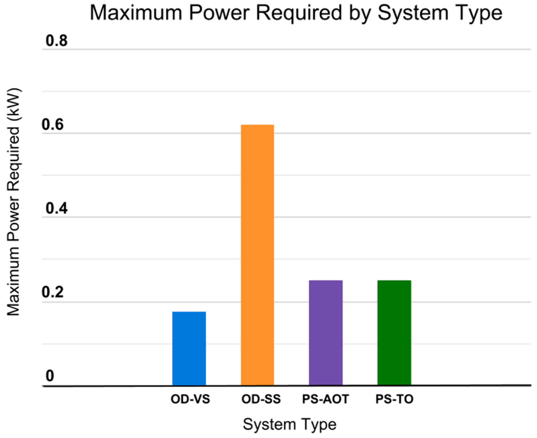
Figure 4.
This figure shows the OD-VS model has a maximum power requirement of 0.18 kW, while the OD-SS model has a maximum power requirement of 0.62 kW, the PS-AOT and the PS-TO models both have a maximum power requirement of 0.25 kW.
Figure 4.
This figure shows the OD-VS model has a maximum power requirement of 0.18 kW, while the OD-SS model has a maximum power requirement of 0.62 kW, the PS-AOT and the PS-TO models both have a maximum power requirement of 0.25 kW.

Figure 5.
This figure shows the OD-SS model requires the highest amount of battery storage (1.65 kWh), and the PS-TO is the lowest (0 kWh). We see the battery storage requirements for the OD-SS, OD-VS and PS-AOT systems are relatively similar due to the UV Lamp energy being the main driver for this storage energy.

Table 1.
Parameters for Equations (4) and (5) specifying parameter, symbol used, value and units used.
Table 1.
Parameters for Equations (4) and (5) specifying parameter, symbol used, value and units used.
| Parameter | Symbol | Value | Unit |
|---|---|---|---|
| Pump Steady State Power per hour | 0.56 | kW | |
| Average Duration per hour | Based on REU2016 Data | seconds | |
| Pump Startup Energy per hour | Determined from Equation (2) | kWh | |
| Power Consumption of UV lamp for 1 hour | 0.060 | kWh | |
| Battery Round-Trip Efficiency | 0.89 | NA |
Table 2.
Parameters for Equations (6) and (7) specifying parameter, symbol used, value and units used.
Table 2.
Parameters for Equations (6) and (7) specifying parameter, symbol used, value and units used.
| Parameter | Symbol | Value | Unit |
|---|---|---|---|
| Hydraulic Head | 15 | meter | |
| Friction Head Loss Coefficient | C | ||
| Average Flow Rate for Hour | Based on REU2016 Data | ||
| Density of Water | 1000 | ||
| Gravitational Constant | 9.81 | ||
| Pump Efficiency | 0.27 | NA |
Table 3.
Parameters for Equation (8) for a variable speed pump, specifying parameter, symbol used, value and units used.
Table 3.
Parameters for Equation (8) for a variable speed pump, specifying parameter, symbol used, value and units used.
| Parameter | Symbol | Value | Unit |
|---|---|---|---|
| Combined Static and Kinetic Pressure Drop | 35.16 (or 50 psi) | meter | |
| Power | 120 | Watts | |
| Flow Rate | Q | 1.5 | GPM |
| Density of Water | 1000 | ||
| Gravitational Constant | 9.81 |
Table 4.
Parameters for Equations (9) and (10) specifying parameter, symbol used, value and units used.
Table 4.
Parameters for Equations (9) and (10) specifying parameter, symbol used, value and units used.
| Parameter | Symbol | Value | Unit |
|---|---|---|---|
| Pump Steady State Power per Hour | Determined from Equation (6) | kW | |
| Average Duration per Hour | Based on REU2016 Data | seconds | |
| Power Consumption of UV lamp for 1 hr | 0.060 | kWh | |
| Battery Round-Trip Efficiency | 0.89 | NA |
Table 5.
Parameters for Equation (11) for a small, medium and large single speed pump specifying parameter, symbol used, value and units used.
Table 5.
Parameters for Equation (11) for a small, medium and large single speed pump specifying parameter, symbol used, value and units used.
| Parameter | Symbol | Value | Unit |
|---|---|---|---|
| Combined Static and Kinetic Pressure Drop | 28 (or 40 psi) | meter | |
| Power | 28.8, 104.5, 123.7 for small, medium and large pumps, respectively. | Watts | |
| Flow Rate | Q | 0.63, 2.54, 3.10 for small, medium and large pumps, respectively | GPM |
| Density of Water | 1000 | ||
| Gravitational Constant | 9.81 |
Table 6.
Parameters for Equation (12) specifying parameter, symbol used, value and units used.
| Parameter | Symbol | Value | Unit |
|---|---|---|---|
| Pressure Head | 30 | meter | |
| Friction Constant | k | meter | |
| Assigned Time Interval | 0.75, 1 and 4 | hours | |
| Density of Water | 1000 | ||
| Gravitational Constant | 9.81 | ||
| Pump Efficiency | 0.38, 0.42 and 0.43 | NA |
Table 7.
Parameters for Equation (13) specifying parameter, symbol used, value and units used.
| Parameter | Symbol | Value | Unit |
|---|---|---|---|
| Pump Steady State Power | Determined by Equation (12) | kW | |
| Assigned Time Interval | 0.75, 1 and 4 | hours | |
| Power of UV Lamp | 0.060 | kW | |
| Battery Round-Trip Efficiency | 0.89 | NA |
Table 8.
Parameters for Equation (14) specifying parameter, symbol used, value and units used.
| Parameter | Symbol | Value | Unit |
|---|---|---|---|
| Pump Steady State Power | Determined by Equation (12) | kW | |
| Assigned Time Interval | 0.75, 1 and 4 | hours | |
| Power of UV lamp | 0.060 | kW |
Table 9.
Energy Calculations for the PS-TO System.
| Symbol | Value | ||||
| 30 | |||||
| C_friction () | 2.51 × 10⁸ | ||||
| Total Volume (m3) | 0.55 | ||||
| 1000 | |||||
| 9.81 | |||||
| (kW) | 0.06 | ||||
| Pump Time (h) | Pump Size | Pump Efficiency | Pump Power (kW) | Total Daily Energy (kWh) | |
| 0.75 | Large | 0.43 | 0.00020 | 0.19 | 0.19 |
| 1 | Medium | 0.42 | 0.00015 | 0.13 | 0.19 |
| 4 | Small | 0.38 | 0.00004 | 0.03 | 0.36 |
Table 10.
Ranges of capacity, price PC and PC average for system components.
| Component | Capacity Range | Price Range | PC Range | PC Avg. |
|---|---|---|---|---|
| Lithium-Ion Batteries | 5.3–31.2 kWh | $6495–$32,975 | $1056–$1225/kWh | $1099/kWh |
| PV Arrays | 2.43–5.97 kWh | $6620–$9559 | $1601–$2724/kWh | $2138/kWh |
| Single Speed Pumps | 560–1491 W | $518–$1390 | $0.71–$1.84/W | $1.04/W |
| Constant Pressure Pumps | 560–1491 W | $1828–$2302 | $1.54–$3.29/W | $2.19/W |
| UV Lamps | 9–40 GPM | $450–$2139 | $45–$71/GPM | $57/GPM |
| Pre-charged Tanks | 86–119 | $696–$940 | $7–$8/gallon | $8/gallon |
Table 11.
Parameters for Equation (16) specifying parameter, symbol used, value and units used.
| Parameter | Symbol | Value | Unit |
|---|---|---|---|
| Over Size Factor | 1.25 | NA | |
| Energy Requirement for System for Daytime Use | Determined by System | kWh | |
| Energy Requirement for System for Nighttime Use | Determined by System | kWh | |
| Battery Price by Capacity Ratio Average | From Equation (15a) | $/kWh | |
| PV Price by Capacity Ratio Average | From Equation (15b) | $/kWh | |
| Pump Power Rating for System | Determined by System | Watts | |
| Pump Price by Capacity Ratio Average | From Equations (15c) or (15d) Depending on pump type | $/Watt | |
| Average Flow Rate | 3 | GPM | |
| UV Lamp Price by Capacity Ratio Average | From Equation (15e) | $/GPM | |
| Volume of Stored Pressurized Water Required | Determined by System | gallons | |
| Pressurized Storage Tank Price by Capacity Average | From Equation (15f) | $/gallon |
Table 12.
Estimated Maximum Price per System using Equation (15).
| System | Estimated Max Price ($) | ||
|---|---|---|---|
| OD-SS | 2.63 | 560 | $5785 |
| OD-VS | 1.65 | 120 | $3519 |
| PS-AOT | 1.69 | 190 | $4562 |
| PS-TO | 0.36 | 190 | $2319 |
See Table A11 in Appendix A for data and calculations per system.
Table 13.
Price Comparisons between systems with OD-SS as a base.
| System | Price Comparison Factor | Percent Decrease |
|---|---|---|
| OD-SS (base) | 1.00 | NA |
| OD-VS | 0.61 | 39% |
| PS-AOT | 0.79 | 21% |
| PS-TO | 0.40 | 60% |
© 2018 by the authors. Licensee MDPI, Basel, Switzerland. This article is an open access article distributed under the terms and conditions of the Creative Commons Attribution (CC BY) license (http://creativecommons.org/licenses/by/4.0/).
Share and Cite
MDPI and ACS Style
Rose, H.S.; Upshaw, C.R.; Webber, M.E. Evaluating Energy and Cost Requirements for Different Configurations of Off-Grid Rainwater Harvesting Systems. Water 2018, 10, 1024. https://doi.org/10.3390/w10081024
AMA Style
Rose HS, Upshaw CR, Webber ME. Evaluating Energy and Cost Requirements for Different Configurations of Off-Grid Rainwater Harvesting Systems. Water. 2018; 10(8):1024. https://doi.org/10.3390/w10081024
Chicago/Turabian StyleRose, Heather S., Charles R. Upshaw, and Michael E. Webber. 2018. "Evaluating Energy and Cost Requirements for Different Configurations of Off-Grid Rainwater Harvesting Systems" Water 10, no. 8: 1024. https://doi.org/10.3390/w10081024
Note that from the first issue of 2016, this journal uses article numbers instead of page numbers. See further details here.