Improved Mixed Distribution Model Considering Historical Extraordinary Floods under Changing Environment

Abstract

Historical extraordinary floods are an important factor in non-stationary flood frequency analysis and they may occur at any time, regardless of whether the environment is changing or not. Based on mixed distribution (MD) modeling, this paper proposed an improved mixed distribution (IMD) model to consider the discontinuity and non-stationarity of flood samples simultaneously, which adds historical extraordinary floods in both sub-series divided by a change point. As a case study, the annual maximum peak discharge and volume series of Ankang hydrological station, located in the upper Hanjiang River Basin of China, were selected to identify non-stationarity by using the variation diagnosis system. MD and IMD were used to fit the flood characteristic series and a genetic algorithm was employed to estimate the optimal parameters. Compared with the design flood values fitted by the stationary Pearson type-III distribution, the results computed by IMD decreased at low return periods and increased at high return periods, with the difference varying from −6.67% to 7.19%. The results highlighted that although the design flood values of IMD are slightly larger than those of MD with different return periods, IMD provided a better result than MD. IMD provides a new perspective for non-stationary flood frequency analysis.

1. Introduction

According to the Intergovernmental Panel on Climate Change (IPCC) Fifth assessment report [1], global warming will be a considerable issue in the future, resulting in subtle changes in the global water cycle and even the global distribution of water. Furthermore, high intensity human activities have resulted in substantial changes in the land surface conditions of many river basins [2], thus affecting the mechanism of runoff generation and convergence in basins. Under the joint influence of the above aspects, the observed hydrological time series have changed substantially, which makes the assumption of “stationarity” questionable in traditional hydrological frequency analysis [3].

Liang et al. [4] grouped non-stationarity flood frequency methods into two types: indirect and direct methods. The indirect methods are mainly based on the rainfall-runoff relation of the basin as well as the decomposition and composition of time series or the hydrological model to revise the hydrological series to eliminate the influence of climate change and human activities and to finally construct stationary time series. A large amount of literature has carried out studies with the indirect methods [5,6,7,8]. However, because the direct methods do not need to restore the hydrological time series, they have been widely used. The direct methods can be divided into three methods: the mixed distribution method, time variant moment method [9,10,11] and conditional probability distribution method [12].

The mixed distribution (MD) method was employed by Singh and Sinclair for the first time [13]. Although this method was widely used in non-stationary flood frequency analysis, parameter estimation is a substantial limit in this method. Alila and Mtiraoui found that the MD model provided a more satisfactory fitting than a traditional single distribution model in the Gila River Basin [14]. Meanwhile, the authors noted that the key to ensuring the accuracy of the MD model lies in two aspects. One aspect is to analyze the formation mechanism of floods in detail and to rationally divide the series of hydrological extremes. In some cases, the sub-distributions were divided by the different causes of floods, such as seasonality [15,16,17], or the change point of the hydrological series [18]. The other aspect is to keep the number of sub-distributions to a minimum, mainly because the increase in sub-distributions will increase the number of parameters and affect the accuracy of the model parameter estimation. Thus, the determination of the estimated parameter is key to the MD model. Various parameter estimation methods were used to address this problem, such as the maximum likelihood method [19], principle of maximum entropy (POME) [20], EM/ECM algorithm [21] and simulated annealing algorithm (SAA) [22]. These examples illustrate that the application of an intelligent optimization algorithm is more and more widely used in parameter estimation and the accuracy of estimation is improved.

Recently, Yan et al. [22] considered the time variability of the parameters in the mixed distribution. The authors proposed the time-varying two-component mixed distributions (TTMD), which considers the time variant in both the weighting coefficients of MD and the parameters of individual component distributions. However, the conventional mixed distributions method often uses the continuous gauged flood sequence as the study sample, without considering historical extraordinary flood data. The historical extraordinary floods refer to the rare extraordinary floods that have occurred in history but were not observed by hydrological stations. The peak discharge of historical extraordinary floods can be attained through historical flood investigation generally. Schendal et al. [23] and Strupczewski et al. [24] showed that the historical extraordinary flood event has a large influence on the calculation accuracy of flood frequency analysis. Taking historical extraordinary flood events into consideration not only increases the information of the flood samples [25,26] but also effectively reduces the uncertainty of flood frequency analysis [27,28]. This idea provides an important reference for the design, operation and management of water conservancy projects. However, due to the addition of historical extraordinary floods, the hydrological series has become a discontinuous series. Many scientists have exploited the employment of historical extraordinary flood data in flood frequency analysis for the last few decades [29,30]. However, the study of considering both historical extraordinary flood events and non-stationarity of flood series is limited. Machado et al. [31] used the time-varying model based on Generalized Additive Models for Location, Scale and Shape (GAMLSS) modelling and incorporated the external covariates to analyze the flood frequency of a 400-year flood record from the Tagus River in Spain, which obtained a better fitting Zeng et al. [18] used the mixed distribution model to handle non-stationarity. The authors divided the series by the change point and added the historical extraordinary flood data into the sub-series before the change point but not in the post-sub-series. In other words, the authors did not consider the influence of historical extraordinary flood events for the sub-series after the change point. However, historical extraordinary flood events are likely to occur at any time, regardless of whether the environment is changing or not.

Therefore, the results of design floods will first be compared in this paper in a variety of cases, such as with or without historical extraordinary floods. The novelty of this paper is to propose an improved mixed distribution (IMD) method, which adds historical extraordinary flood events in both sub-series divided by a change point. As case studies, the proposed IMD method will be applied to the Ankang hydrological station in the upper stream of the Hanjiang River Basin, China, where many extraordinary floods have occurred in history. A genetic algorithm will be employed to estimate the optimal parameters. The change in the design flood under different return periods will be compared and analyzed, which will provide a new method for non-stationarity flood frequency analysis considering historical extraordinary flood events.

2. Materials and Methods

2.1. Variation Diagnosis System

The time series of hydrological variables can reflect the extent of the hydrological variables affected by climatic conditions and human activities. There are many methods to test the variation of the hydrological series but there is often a problem in that the results of various methods are not consistent. The hydrological variation diagnosis system, proposed by Xie et al. [32], can be divided into three procedures: primary diagnosis, detailed diagnosis and comprehensive diagnosis, which makes the results more objective and reasonable. A variety of corresponding methods can be used at each procedure of diagnosis. Finally, the results of comprehensive diagnosis can be obtained by combining the weight synthesis.

In this study, we use the Hurst exponent [33] as the method of primary diagnosis to test the degree of variation for each series. According to the calculated Hurst exponent value and the classification of variation degree shown in

Table 1. Classification of variation degree.

Correlation Function C(t)	Hurst Exponent h	Variation Degree
$0\le C(t)<r_{\alpha }$	$0.5\le h<h_{\alpha }$	No variation or Weak variation
$r_{\alpha }\le C(t)<0.6$	$h_{\alpha }\le h<0.839$	Medium variation
$0.6\le C(t)<0.8$	$0.839\le h<0.924$	Strong variation
$0.8\le C(t)\le 1.0$	$0.924\le h\le 1.0$	Vast variation

where $\alpha$ is significance level, $r_{\alpha }$ denotes the correlation function C(t) corresponding to $\alpha$ significance level, C(t) = 2^2h−1 − 1; $h_{\alpha }=\frac{1}{2}\left[1+\ln (1+r_{\alpha })/\ln 2\right]$.

[32], the variation degree of each series can be determined. For the detailed diagnosis, we propose the Spearman and Kendall rank correlation coefficient methods [34,35] to investigate the trends. The Lee-Heghinian method [36], Sequential clustering method [37], Pettitt test [38], Mann-Kendall test [39,40] and R/S analysis method [33] are used to identify the change points of the series. Combined with the hydrological survey investigation and detailed diagnosis results, a final comprehensive diagnosis can be conducted.

2.2. Mixed Distribution Model

2.2.1. Mixed Distribution

The mixed distribution model was first proposed by Singh and Sinclair and applied to the non-stationary hydrological frequency analysis [13]. This model can be defined as a probability distribution composed of multiple sub-series distributions; that is, its cumulative distribution function can be regarded as a linear distribution of cumulative distribution functions of several sub-series distributions. The expression is shown in Equation (1).

$$F(x)=w_1{F}_1(x)+w_2{F}_2(x)+\cdots +w_k{F}_k(x)$$

(1)

where $w_i$ is the weighting coefficient of each sub-series distribution and satisfies the equation of $w_i>0$ and ${\displaystyle \sum _{i=1}^k{w}_i=1}$. The number of sub-series distribution is denoted as k. $F_k(x)$ denotes the cumulative distribution functions of each sub-series distributions.

Certainly, the weighted average of cumulative distribution functions is not the only way to cope with the multiple components series. Strupczewski et al. [41] provided a seasonal approach to flood frequency analysis. Kochanek et al. [42] applied this approach to the annual peak flow series of Polish rivers, which are formed from summer and winter flows. The method showed that seasonal cumulative distribution functions can also provide good results.

The number of sub-series distributions of mixed distribution can often be determined by the hydrological variation diagnosis results or the physical mechanism of floods. In most cases, to reduce the complexity of mixed distribution, two-component mixture models were often used. For example, Waylen and Woo noted that the simple Gumbel distribution does not fit the different flood-generating processes well [15]; they divided the observed annual flood series data into two subsets (the snowmelt flood and the rainfall flood) and fitted it by using mixed distribution. Zeng et al. [18] divided the annual flood series into two components according to the change points based on the variation diagnosis results.

Thus, we also divide the flood series into two sub-series according to the variation diagnosis results. In China, Pearson type-III (P3) is recommended for flood frequency analysis according to the Regulation for Calculating Design Flood of Water Resources and Hydropower Projects [43]. In this paper, we assume each sub-series distribution is subject to a P3 distribution, denoted as $f_1(x)$ and $f_2(x)$, respectively. The whole mixed distribution model is given by

$$\{\begin{array}{l}f(x)=w{f}_1(x)+(1-w)f_2(x)\\ f_1(x)=\frac{{\beta }_1{}^{{\alpha }_1}}{\mathsf{\Gamma }({\alpha }_1)}{(x-a_{01})}^{{\alpha }_1-1}{e}^{-{\beta }_1(x-a_{01})}\\ f_2(x)=\frac{{\beta }_2{}^{{\alpha }_2}}{\mathsf{\Gamma }({\alpha }_2)}{(x-a_{02})}^{{\alpha }_2-1}{e}^{-{\beta }_2(x-a_{02})}\end{array}$$

(2)

where $w$ is the weighting coefficient of mixed distribution. ${\alpha }_i$, ${\beta }_i$ and $a_{0i}(i=1,2)$ denote the shape, scale and location parameter of the probability density function $f_i(x)$ of each sub-series distribution, respectively. In flood frequency analysis, these three parameters can be expressed by mean EX_i, variation coefficient C_vi and skewness coefficient C_si. The formulas are given as follows: $a_{0i}=E{X}_i(1-\frac{2C_{vi}}{C_{si}})$, ${\alpha }_i=\frac{4}{C_{si}{}^2}$ and ${\beta }_i=\frac{2}{E{X}_i{C}_{vi}{C}_{si}}$. The initial value of the sample mean EX₁ and EX₂ estimated by the moment method can be considered as the unbiased estimate of the total. Thus, there are w, C_v1, C_v2, C_s1 and C_s2 up to five parameters to be estimated in mixed distribution f(x).

2.2.2. Parameter Estimation

Zhao et al. [44] proposed a curve fitting method for P3 with discontinuous series considering historical extraordinary flood data by using the genetic algorithm (GA), illustrating that the genetic algorithm has good global search ability and can reduce the error of fitting. To fit the empirical frequency points of historical extraordinary flood data, the theoretical frequency curve should pass through the center of the point group of the historical extraordinary flood data and the measured flood data. Hence, we fitted discontinuous series considering historical extraordinary flood data by weight and estimated the optimal parameters for a mixed distribution by using GA. The weight of the historical extraordinary flood data is denoted p, the weight of the measured flood data is denoted q and the formula is shown in Equation (3). Thus, the weighted least square (WLS) method was applied to construct the objective function with the weight coefficient, which is shown in Equation (4).

$$p=\frac{n-l}{a+n};q=1-p=\frac{a+l}{a+n}$$

(3)

$$S_{WLS}(EX,C_v,C_s)=p{{\displaystyle \sum _{j=1}^{a+l}[\frac{x_j-f(P_j,EX,C_v,C_s)}{x_j}]}}^2+q{{\displaystyle \sum _{i=1}^{n-l}[\frac{x_i-f(P_i,EX,C_v,C_s)}{x_i}]}}^2$$

(4)

where a is the number of historical extraordinarily large floods, n is the number of the measured flood series and l is the number of extraordinary large floods from the measured flood series.

During the iterative process, we first estimate the mean value for the two sub-series by the moment method. Then, the genetic algorithm is employed to optimize the other five parameters for mixed distributions, that is, w, C_v1, C_v2, C_s1 and C_s2, which can make the objective function attain the minimum and obtain the best fitted mixed distribution parameters. The main calculation procedures are as follows.

(1)

Use real number coding to generate an initialization population with a population size Np of 100. The initial parameter variation range of five parameters for mixed distribution should be constrained. For example, the weight coefficient w of each sub-series distribution should be between 0~1, the variation range of C_v should be 0~2 according to the information of the Ankang hydrological station and the variation range of C_s/C_v should be between 2~2.5. This approach effectively avoids the large deviation between the estimated values of C_v and C_s/C_v as well as the recommended value.

(2)

Calculate the fitness of the initial population. The fitness value of the initial population can be calculated through the objective function shown in Equation (4).

(3)

Set the population gap GGAP = 0.7, the crossover probability P_c = 0.6 and the maximum number of iterations N_G = 150; the processes of multiple selection, crossover and mutation are carried out for the initial population. Each iteration is used to evaluate the fitness of the population to minimize the objective function value until the optimal parameter is obtained according to the maximum number of iterations.

2.2.3. Model Evaluation Criterion and Goodness-of-Fit Test

The Kolmogorov-Smirnov (K-S) goodness-of-fit test [45] and the AIC criterion [46] were used to test the fitting of each series. The K-S test statistic D is given by

$$D=\underset{-\infty <x<+\infty }{\max }\left|F_n(x)-F_0(x)\right|$$

(5)

where $F_n(x)$ denotes the cumulative distribution function of random samples, that is, the empirical frequency of the series. $F_0(x)$ denotes the distribution form to be tested, that is, the theoretical frequency. n is the sample size and $\alpha$ is the significance level. If the value of statistic D is less than or equal to the critical value $D_n(\alpha )$, then the original hypothesis is accepted and it is considered that the fitting is good according to the test. The AIC criterion is also used to evaluate the goodness of fit, which is given by

$$MSE=\frac{1}{n}{\displaystyle \sum _{i=1}^n{(P{e}_i-P_i)}^2}$$

(6)

$$AIC=n\ln (MSE)+2m$$

(7)

where $P{e}_i$ and $P_i$ denotes the empirical frequency and theoretical frequency of the series, respectively. m is the number of frequency distribution parameters. Taking P3 distribution as an example, there are EX, C_v and C_s up to three parameters in the P3 distribution; thus, m = 3.

2.3. Improved Mixed Distribution Model

We propose the IMD model based on the methods of MD. Because historical extraordinary floods may occur before and after the change in land surface, we take historical extraordinary floods into both sub-series, which are divided by the change point. Thus, both sub-series are discontinuous and are formed with the observed data and historical data. Compared with the MD model, the sub-series before the change point should use moment estimation of the discontinuous sample mean and the sub-series after the change point is necessary for using the same method to calculate the mean value. The change in the mean value is the key difference between the IMD model and MD. The estimation methods of the other parameters are the same. The formula of moment estimation of the discontinuous sample mean is given as follows.

$$\overline{EX}=\frac{1}{N}[{\displaystyle \sum _{i=1}^{a}E{X}_i+\frac{N-a}{n-l}{\displaystyle \sum _{j=l+1}^{n}E{X}_j}}]$$

(8)

where $\overline{EX}$ represents the mean of the discontinuous sample. N is the recurrence period of the historical extraordinary flood. $a$ is the number of historical extraordinary floods. l represents the number of historical extraordinary floods in the observed series.

2.4. Monte Carlo Simulation

In this work, in order to test whether the length of data will affect the results of design flood values at high return periods, we verify our design flood results via Monte Carlo simulation [47]. According to the moment method, the initial value of sample mean EX, variation coefficient $C_v$ and skewness coefficient $C_s$ for hydrological series can be obtained. Based on the initial parameters, we can use the Monte Carlo method to generate synthetic data with a length of 10,000, which obey the P3 distribution. According to the optimized parameters by GA, theoretical frequency series of observed data can be calculated. To investigate the variation of the synthetic data and the results of observed data, normalized mean bias (NMB) [48] and relative root mean square error (RRMSE) [49] statistical parameters are used for comparison. The formula is given as follows.

$$NMB=\frac{\frac{1}{n}{\displaystyle \sum _{i=1}^n(x_O-x_{MC})}}{\frac{1}{n}{\displaystyle \sum _{i=1}^n{x}_{MC}}}\mathrm{v}$$

(9)

$$RRMSE={\left[\frac{1}{n}{\displaystyle \sum _{i=1}^n{(\frac{x_O-x_{MC}}{x_{MC}})}^2}\right]}^{1/2}$$

(10)

where n is the length of synthetic data, which is 10,000. $x_O$ represents the design flood values of the observed series estimated by GA. $x_{MC}$ represents the design flood values of synthetic data generated by the Monte Carlo method. Note that lower NMB and RRMSE represent a better performance.

In addition, in order to estimating the uncertainties, nonparametric bootstrap method is used to determine the confidence intervals for flood frequency curves. Nonparametric bootstrap method is resampling from the original data to obtain the bootstrapped sample of flood data.

3. Study Area and Data Set

3.1. Study Area

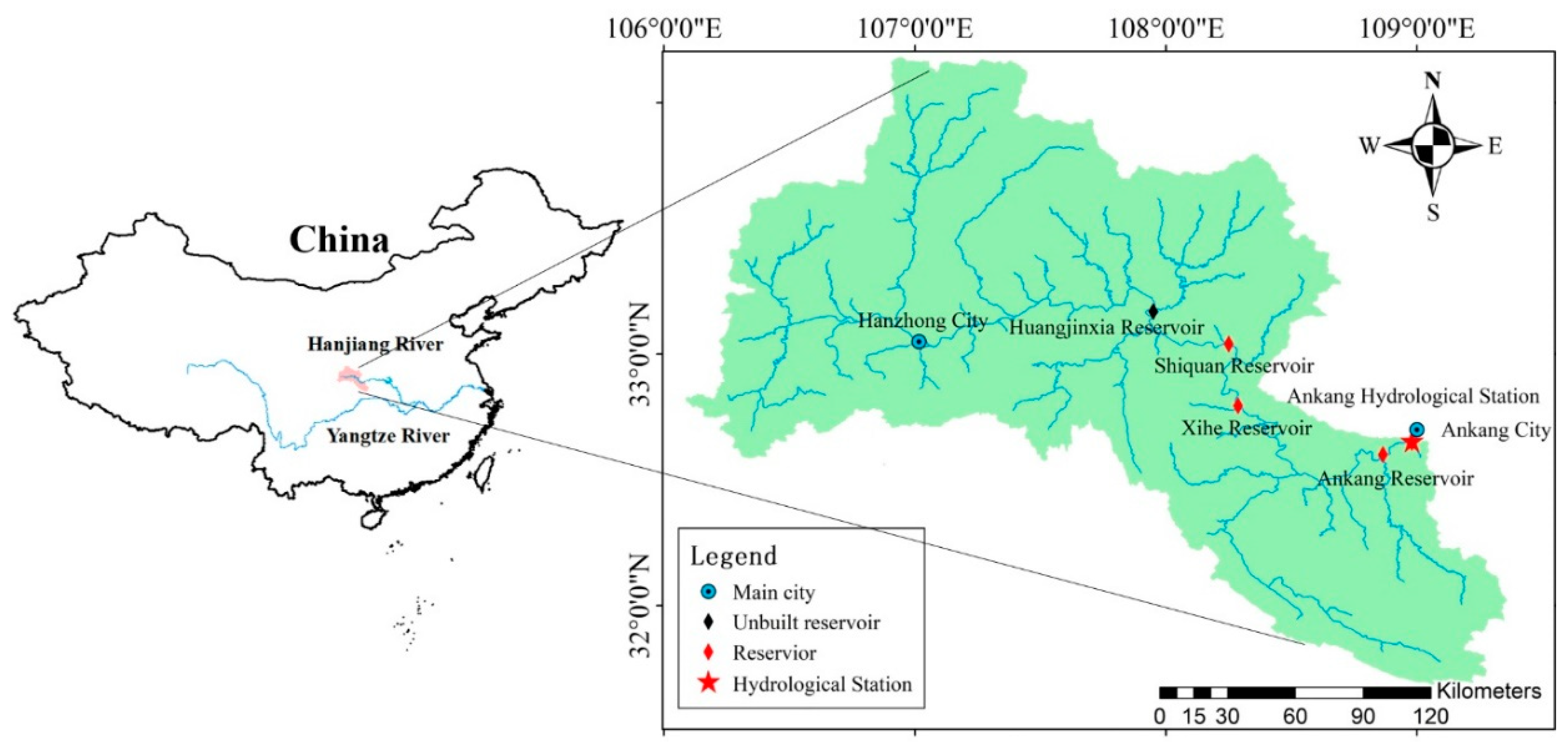
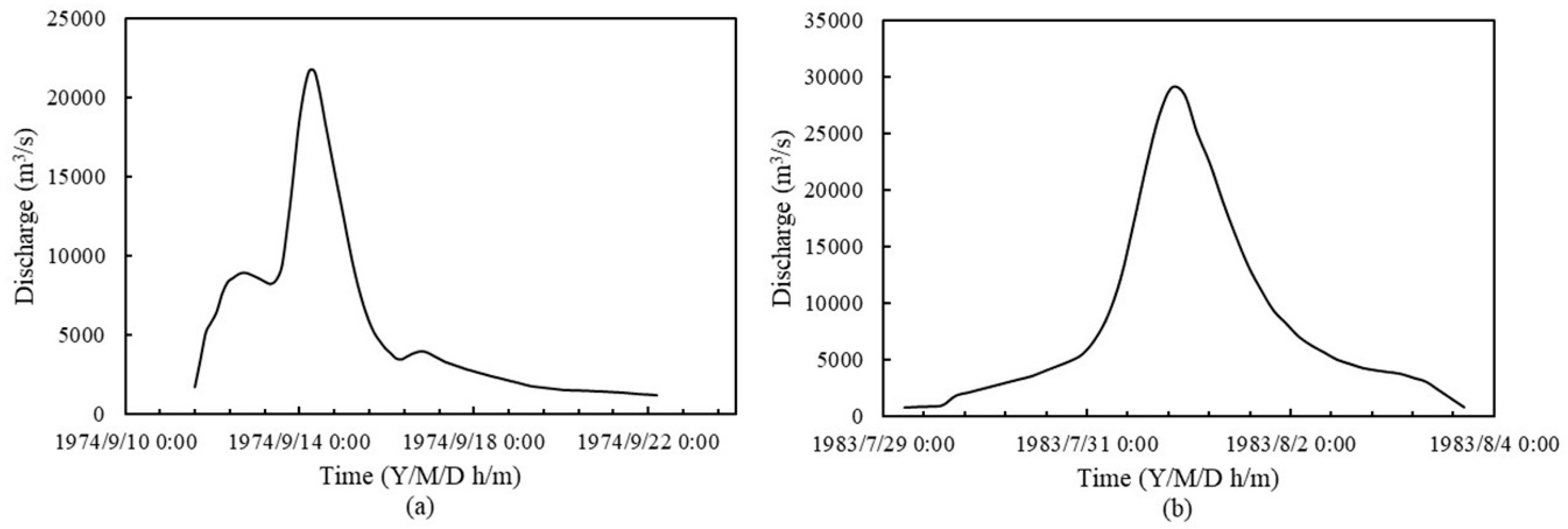
The Hanjiang River is one of the largest tributaries of the Yangtze River in China, with a catchment area of 159,000 km² and a length of 1570 km. The basin is bounded by 30°10′ N to 34°20′ N latitude and 106°15′ E to 114°20′ E longitude. Originating in Hanzhong city of Shaanxi province, the main stream flows southeast through Shaanxi and Hubei provinces and returns to the Yangtze River in Wuhan city. The area controlled by the Ankang hydrological station, with a catchment area of 38,700 km², is the study area (shown in Figure 1). The annual average discharge is 621 m³/s at the Ankang hydrological station. The study area has a subtropical continental monsoon climate, which is mild and has four distinctive seasons. The average annual temperature is 15~17 °C and the annual average rainfall is 800~1000 mm. Floods are mainly caused by rainfall, occurring over 3~10 months but mostly in summer and autumn. Summer floods mainly occur in July, mostly consisting of a heavy intensity and short duration rainstorms. Autumn floods often appear in September, generally consisting of stable and persistent rainfall. Thus, the floods in autumn often have a long duration and large volume. The hydrographs of the 1974 typical flood and the 1983 largest flood are shown in Figure 2.

Several reservoirs have been built in this drainage area for the purposes of flood control, irrigation and electricity generation [50]. The geographical distribution of these reservoirs at the upper reaches of the Ankang hydrological station is shown in Figure 1. The information for the reservoirs is shown in

Table 2. Information for the reservoirs in the study area.

Name of Reservoir	Drainage Area (km2)	Annual Average Flow (m3/s)	Design Flood Flow (m3/s)	Storage Capacity (108 m3)	Completion Year
Huangjinxia	17,950	259	18,000	0.92	Not built yet
Shiquan	23,400	343	21,500	1.80	1974
Xihe	25,207	361	21,800	0.20	2006
Ankang	35,700	621	36,700	14.72	1992

.

3.2. Data Set

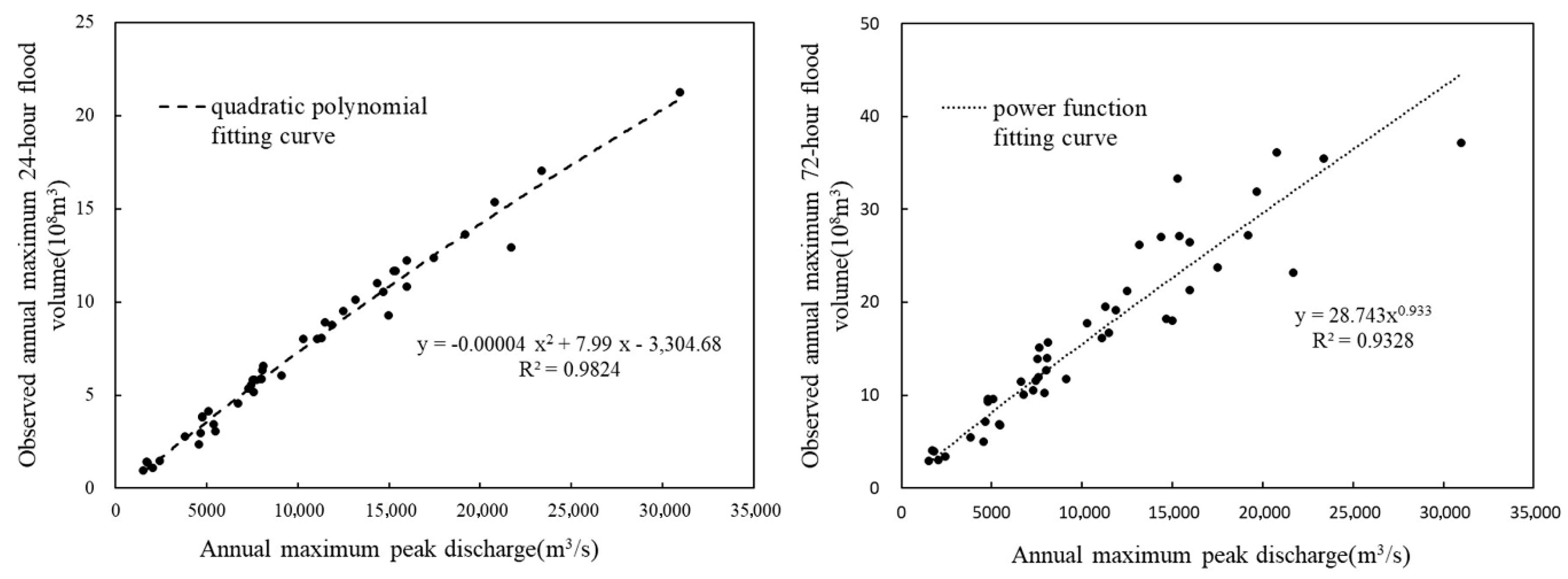
In this study, the hourly observed flood data during the period of 1968–2013 at the Ankang hydrological station were available and the series during the annual maximum peak discharge series (AMPDS), annual maximum 24-h flood volume series (24-h AMFVS) and annual maximum 72-h flood volume series (72-h AMFVS) between 1968–2013 were selected. Among them, the flood in July of 1983 with a peak discharge of 31,000 m³/s is the largest flood that has been encountered since the establishment (1935) of the Ankang hydrological station. In addition, combined with the historical extraordinary floods investigation results by Yang [51,52], the historical extraordinary flood data of 36,000 m³/s in 1583, 30,000 m³/s in 1867 and 26,000 m³/s in 1921 were selected. Due to the lack of historical extraordinary flood volume data, the correlation relationship (shown in Figure 3) between the flood peak and volume of the Ankang hydrological station was used to calculate the historical maximum 24-h and 72-h flood volume data corresponding to the historical maximum peak discharge. The three series of flood samples that consider the discontinuity of historical extraordinary floods are formed.

4. Results and Discussion

4.1. Results of the Variation Diagnosis System

4.1.1. Primary Diagnosis

The Hurst exponent h values of the flood characteristics series of the Ankang hydrological station for 1968~2013 were calculated and the variation degree was determined according to the classification of variation degree shown in Table 1. The results are shown in

Table 3. Calculation results of the Hurst exponent for each flood characteristic series.

Flood Characteristics Series	Hurst Exponent	$\mathit{C}(\mathit{t})$	Variation Degree
AMPDS	0.8047	0.5256	Medium variation
24-h AMFVS	0.7352	0.3855	Medium variation
72-h AMFVS	0.8107	0.5384	Medium variation

. AMPDS, 24-h AMFVS and 72-h AMFVS all exhibit medium variation, which requires further detailed diagnosis.

4.1.2. Detailed Diagnosis

First, we used the Spearman and Kendall rank correlation coefficient methods to investigate the trends in the three flood characteristics series and then adopted the Lee-Heghinian method, Sequential clustering method, Pettitt test, Mann-Kendall test and R/S analysis method to identify the change points in the series. With a 5% significance level, the critical values of the Spearman and Kendall rank correlation statistics were 2.015 and 1.96, respectively. If the absolute value of the statistics exceeds the critical value, it illustrates that the trend component is significant. The positive and negative values of the statistics show that the trends of the series are increasing or decreasing. From the results, as shown in

Table 4. Detailed diagnosis results.

Variation Component	Methods	AMPDS	24-h AMFVS	72-h AMFVS
Trends	Spearman rank correlation statistics	−2.318	−2.225	−2.384
	Kendall rank correlation statistics	−2.320	−2.452	−2.566
Change point	Lee-Heghinian method	1987	1987	1985
	Sequential clustering method	1987	1987	1985
	Pettitt test	1993	1994	1994
	Mann-Kendall test	1990	1989	1988
	R/S analysis method	1987	1987	1987
	Possible change points	1987	1987	1985 and 1987

, we can learn that the statistics of the two trend analysis methods were negative and the three flood characteristic series have a significant downward trend at the 0.05 significant level. Furthermore, the change points in the flood characteristic series occur between the end of the 1980s and the early 1990s.

4.1.3. Comprehensive Diagnosis

Table 4 illustrates that the possible change point of AMPDS and 24-h AMFVS are in 1987 but the possible change point of 72-h AMFVS appears in 1985 and 1987, which is in accordance with the results of Xiong et al. [53]. Ankang reservoir construction was started in 1978. It began to store water in 1989 and was finished in 1992. These authors considered that the change point was closely linked with the construction of the Ankang reservoir. Zhang et al. [2] compared the catchment runoff change during 2001–2010 with the previous 40 years (1960–2000) and noted that the decrease in runoff in the Hanjiang River Basin was mainly due to the significant change in the land surface conditions. In addition, since there are many dam-break floods that inundated the urban areas of Ankang City, water conservancy projects such as reservoirs and dams began to be built to control floods in the 1980s. Especially after the extraordinary floods that occurred in July of 1983, causing serious economic losses, a ten-mile-long dyke began thorough renovation and was completed in 1987. Therefore, the fact that the change points of the three flood characteristic series, AMPDS, 24-h AMFVS and 72-h AMFVS, are all in 1987 is reasonable.

We also used the Kendall rank correlation coefficient method to investigate the trend for the flood series before the change point (1968–1986) and after the change point (1987–2013). The results are shown in

Table 5. Kendall rank correlation statistic values for the flood series before and after the change point.

Flood Characteristics Series	Kendall Rank Correlation Statistic U
	1968–1986	1987–2013
AMPDS	1.224	−0.063
24-h AMFVS	0.735	−0.271
72-h AMFVS	0.734	−0.229

U represents the Kendall rank correlation statistic. With a 5% significance level, the critical value of Kendall rank correlation statistics was 1.96. If the absolute value of the statistic exceeds the critical value, it illustrates that the trend component is significant. The positive and negative values of the statistics show that the trends of the series are increasing or decreasing.

. From the results, we can see that both trend component of the flood series before and after the change point is not significant. In addition, the trend of flood series before the change point is increasing and the trend of flood series after the change point is decreasing. Thus, the results also verified that the change point is 1987.

Due to the fact that the trends and change point of each flood characteristic series are all significant, the final variation form is determined by calculating the efficiency coefficient, which is given by

$$R^2=1-\frac{{\displaystyle \sum _{i=1}^n{(Q_{obs,i}-Q_{sim,i})}^2}}{{\displaystyle \sum _{i=1}^n{(Q_{obs,i}-{\overline{Q}}_{obs})}^2}}$$

(11)

where $Q_{obs,i}(i=1,2,\cdots ,n)$ is the observed hydrological series. ${\overline{Q}}_{obs}$ denotes the mean value of the observed hydrological series. For the trend component, $Q_{sim.i}(i=1,2,\cdots ,n)$ is the fitted value of each point on the trend line. ${\tau }_i$ denotes the change point of the flood characteristic series and the formula of $Q_{sim,i}$ is expressed by

$$Q_{sim,i}=\frac{1}{{\tau }_i}{\displaystyle \sum _{i=1}^{{\tau }_i}{Q}_{obs,i}(i=1,2,\cdots ,{\tau }_i)}$$

(12)

$$Q_{sim,i}=\frac{1}{n-{\tau }_i}{\displaystyle \sum _{i={\tau }_i+1}^n{Q}_{obs,i}(i={\tau }_i+1,\cdots ,n)}$$

(13)

As

Table 6. Calculation results of the efficiency coefficients.

Flood Characteristic Series	Trend Variation Efficiency Coefficients	Change Point Efficiency Coefficients	Final Variation Forms
AMPDS	0.0857	0.2272	Change point
24-h AMFVS	0.1032	0.2346	Change point
72-h AMFVS	0.1051	0.2202	Change point

shows, the efficiency coefficients of the change points of the flood characteristic series are all larger than those of the trend variation; thus, the final variation forms of all flood characteristic series are change points and the possible change point is 1987.

4.2. Results of Monte Carlo Simulation and Uncertainty Analysis

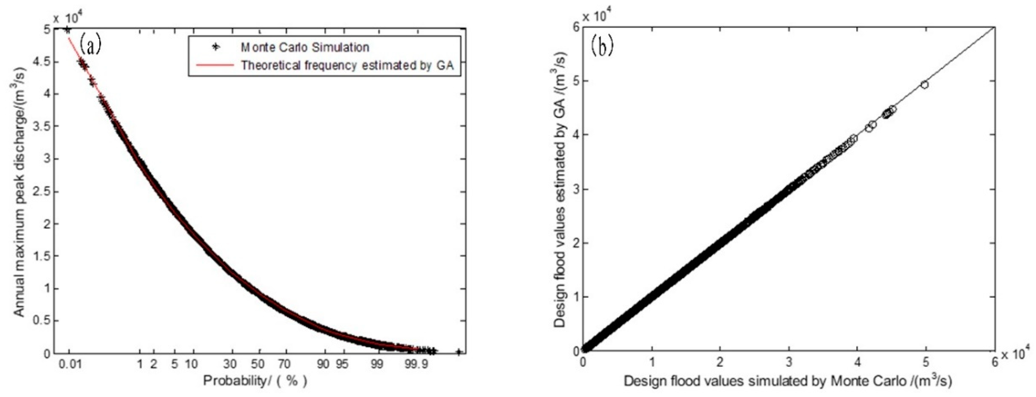
Taking the observed 1968–2013 flood characteristic series with four historical extraordinary flood events as an example, we compared the variation between the design flood value results simulated by Monte Carlo method and estimated by GA. Values of NMB and RRMSE statistical parameters are shown in

Table 7. Values of statistical parameters for all flood characteristic series.

Statistical Parameters	AMPDS	24-h AMFVS	72-h AMFVS
NMB	0.0046	0.0157	0.0208
RRMSE	0.0091	0.0217	0.0281

Lower NMB and RRMSE represent a better performance.

. Figure 4 shows the variation between the design flood values of AMPDS. It illustrates that there is little deviation between the Monte Carlo simulated design flood values and the estimated design flood values by observed flood series. The Monte Carlo simulation of AMPDS exhibited the best results. The statistical parameters of 24-h AMFVS and 72-h AMFVS are slightly larger than AMPDS. It is mainly because the peak discharge of historical extraordinary floods is obtained through historical flood investigation. The historical flood volume data were obtained according to the peak volume relationship of flood, which adds some deviations. However, the statistical parameters are still within the acceptable range. This indicates that we can use 50-year-long datasets including historical extraordinary floods to estimate the design flood values at high return periods.

To estimate the uncertainties for flood characteristic series, nonparametric bootstrap method was used to calculate the 95% confidence interval for flood frequency curve. We obtained a bootstrapped sample from the original flood data with the length of 2000. Figure 5 shows the 95% confidence interval for flood characteristic series.

4.3. Analysis of the Design Flood Results under Changing Environments

Combined with the results of the change point diagnosis, the flood characteristic series can be divided into two sub-series: the observed series before the change point and the observed series after the change point. Taking historical extraordinary flood data into consideration, we designed four cases fitting the P3 distribution to analyze the difference in the design flood under changing environmental conditions, which are as follows.

• Case 1: original flood characteristic series (1968–2013) that do not consider the variation but add the historical extraordinary flood data, denoted as series $A_{i1}$.
• Case 2: observed flood characteristic series before the change point (1968–1987) with the addition of the historical extraordinary flood data, denoted as series $A_{i2}$.
• Case 3: observed flood characteristic series after the change point (1987–2013) with the addition of the historical extraordinary flood data, denoted as series $A_{i3}$.
• Case 4: only the observed flood characteristic series after the change point (1987–2013), denoted as series $A_{i4}$.

Where $i=1,2,3$ represents the AMPDS, 24-h AMFVS and 72-h AMFVS, respectively.

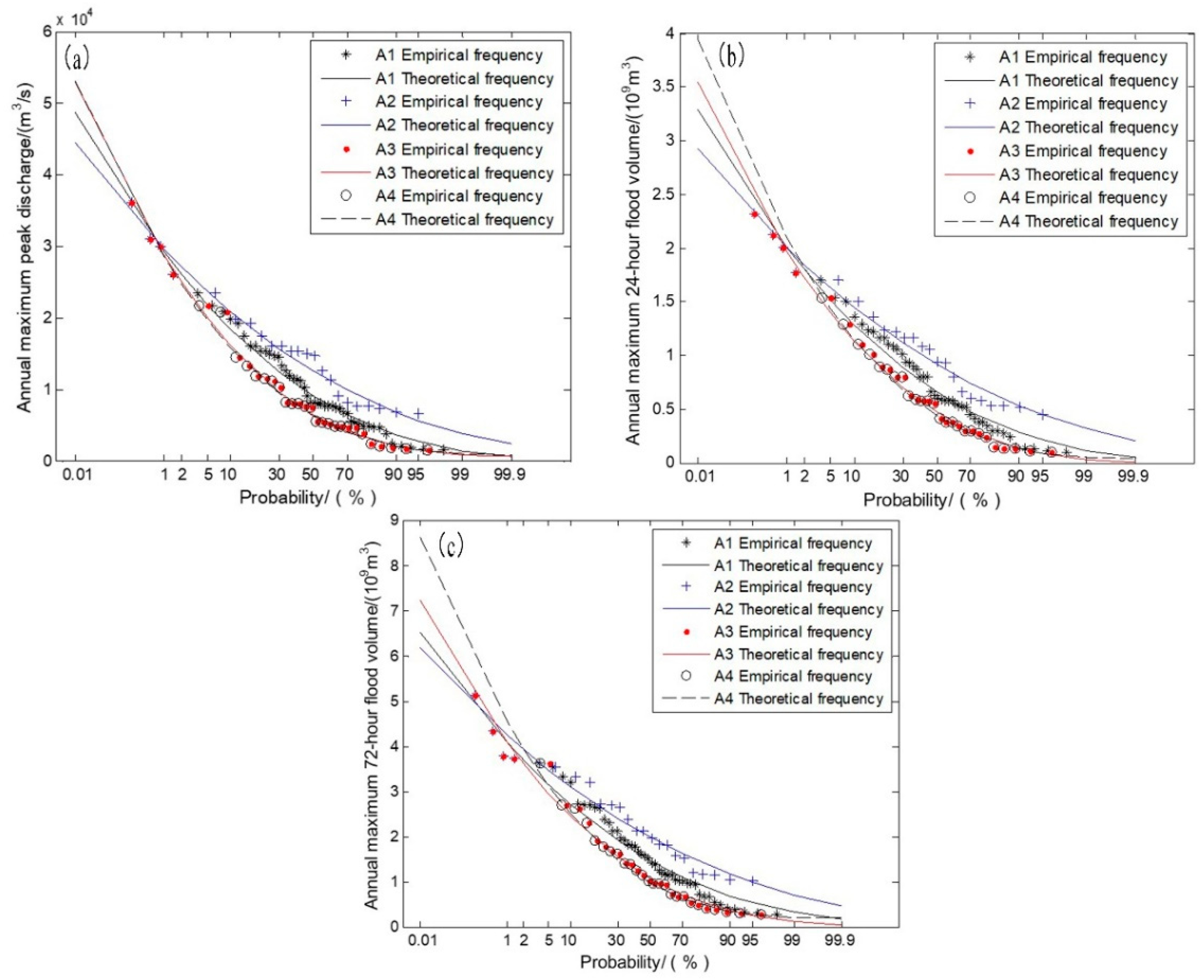
The design floods at different return periods of each flood characteristic series are calculated separately for the four different cases. The genetic algorithm is also used to estimate the parameters of the P3 distribution for the flood series.

Table 8. Results of the estimated parameters for all flood series.

Estimated Parameters	AMPDS (m3/s)				24-h AMFVS (108 m3)				72-h AMFVS (108 m3)
	${\mathit{A}}_{11}$	${\mathit{A}}_{12}$	${\mathit{A}}_{13}$	${\mathit{A}}_{14}$	${\mathit{A}}_{21}$	${\mathit{A}}_{22}$	${\mathit{A}}_{23}$	${\mathit{A}}_{24}$	${\mathit{A}}_{31}$	${\mathit{A}}_{32}$	${\mathit{A}}_{33}$	${\mathit{A}}_{34}$
EX	10,226	13,278	7995	7782	7.35	9.59	5.71	5.57	16.02	20.70	12.60	12.32
Cv	0.59	0.42	0.76	0.77	0.56	0.38	0.72	0.8	0.51	0.37	0.69	0.77
Cs/Cv	2	2	2.15	2.21	2	2	2	2.17	2	2	2.03	2.35

EX denotes the mean value of the series. Cv denotes the variation coefficient. Cs/Cv denotes the ratio of skewness coefficient Cs and the variation coefficient Cv.

shows the results of the estimated parameters for all flood series.

Table 9. Goodness-of-fit test results for all flood series.

Evaluation Indicators	AMPDS				24-h AMFVS				72-h AMFVS
	${\mathit{A}}_{11}$	${\mathit{A}}_{12}$	${\mathit{A}}_{13}$	${\mathit{A}}_{14}$	${\mathit{A}}_{21}$	${\mathit{A}}_{22}$	${\mathit{A}}_{23}$	${\mathit{A}}_{24}$	${\mathit{A}}_{31}$	${\mathit{A}}_{32}$	${\mathit{A}}_{33}$	${\mathit{A}}_{34}$
$D_n(\alpha )$	0.1940	0.2796	0.2400	0.2640	0.1940	0.2796	0.2400	0.2640	0.1940	0.2796	0.2400	0.2640
D	0.0831	0.1571	0.0912	0.1051	0.0881	0.1375	0.0741	0.0928	0.1035	0.1411	0.0615	0.0708
AIC	−313.5	−119.4	−195.2	−156.0	−291.4	−118.2	−200.3	−165.0	−279.4	−126.9	−204.9	−179.6

D denotes the K-S test statistic. $D_n(\alpha )$ is the critical value of K-S test statistic D and D less than $D_n(\alpha )$ means the distribution passes the goodness-of-fit test at the 5% significant level.

illustrates that the results all pass the goodness-of-fit test and the fitting results are shown in Figure 6. According to the optimized parameters obtained, the design values of each flood characteristic series are calculated as shown in

Table 10. Design value of each flood characteristic series.

Flood Characteristic Series		Return Periods in Years
		10,000	5000	1000	500	300	200	100	20	5
AMPDS (m3/s)	1999 design report	48,100	45,500	39,300	36,700	34,600	32,800	30,000	23,000	16,100
	$A_{11}$	48,640	45,802	39,106	36,165	33,971	32,210	29,152	21,730	14,662
	Difference (1) (%)	1.1	0.7	−0.5	−1.5	−1.8	−1.8	−2.8	−5.5	−8.9
	$A_{12}$	44,466	42,340	37,270	35,016	33,320	31,950	29,550	23,579	17,604
	$A_{13}$	52,927	49,325	40,912	37,262	34,559	32,405	28,699	19,939	12,066
	$A_{14}$	53,001	49,339	40,794	37,093	34,354	32,173	28,427	19,601	11,733
	Difference (2) (%)	19.0	16.5	9.8	6.4	3.7	1.4	−2.9	−15.4	−31.5
	Difference (3) (%)	0.1	0.0	−0.3	−0.5	−0.6	−0.7	−0.9	−1.7	−2.8
24-h AMFVS (108 m3)	$A_{21}$	32.98	31.11	26.69	24.75	23.29	22.13	20.10	15.15	10.40
	$A_{22}$	30.00	28.63	25.36	23.90	22.80	21.91	20.35	16.45	12.52
	$A_{23}$	35.47	33.14	27.69	25.32	23.55	22.15	19.72	13.93	8.63
	$A_{24}$	39.80	37.01	30.50	27.69	25.61	23.95	21.10	14.42	8.49
	Difference (2) (%)	18.2	15.8	9.2	5.9	3.3	1.1	−3.1	−15.3	−31.0
	Difference (3) (%)	12.2	11.7	10.2	9.4	8.7	8.1	7.0	3.5	−1.7
72-h AMFVS (108 m3)	$A_{31}$	65.07	61.57	53.28	49.62	46.88	44.67	40.82	31.39	22.19
	$A_{32}$	61.79	59.07	52.55	49.64	47.44	45.66	42.54	34.70	26.72
	$A_{33}$	72.32	67.71	56.91	52.20	48.69	45.89	41.05	29.46	18.73
	$A_{34}$	86.21	80.13	65.97	59.86	55.33	51.74	45.57	31.13	18.41
	Difference (2) (%)	17.0	14.6	8.3	5.2	2.6	0.5	−3.5	−15.1	−29.9
	Difference (3) (%)	19.2	18.3	15.9	14.7	13.6	12.7	11.0	5.7	−1.7

Difference (1) represents the difference percentage in $A_{i1}$ compared with 1999 design report results, difference (2) represents the difference percentage in $A_{i3}$ compared with $A_{i2}$ and difference (3) represents the difference percentage in $A_{i4}$ compared with $A_{i3}$.

.

As shown in Table 10, we learn that the design flood results of $A_{11}$, which considered historical extraordinary flood data but not non-stationary data, are larger than the 1999 design flood results of the Ankang hydrological station at 10,000-year and 5000-year return periods. However, the $A_{11}$ design flood results are smaller at other return periods and the difference is between −8.9% and 1.1%. Compared with the design AMPDS results of the 1999 design report, the design flood of $A_{i1}$, which does not consider the non-stationarity of the series, tends to be larger at a high return period and smaller at a low return period, which may be caused by the increase of the sample size. Mainly because of the decreasing trend of the mean value for the flood characteristic series, the addition of data increases the $C_V$ of the computed series, resulting in the increase in the upper tail of the frequency curve and the decrease in the lower tail.

In the same way, it can be clearly seen that the design values after the change point of the three flood characteristic series $A_{i3}$, considering the historical extraordinary flood data, are smaller than the design values of $A_{i2}$ at 100-year, 20-year and 5-year return periods. For the other return periods, the design values are larger. The difference range of AMPDS is −31.5% to 19.0%, the difference of 24-h AMFVS ranges from −31.0% to 18.2% and the difference of 72-h AMFVS is 29.9% to 17.0%. It can be seen from Fig. 6 that the design flood value, without considering the variation of flood series, is almost between the design values before and after the variation series.

Comparing the design flood results between case 3 and case 4 shows that the $A_{i4}$ design values of 24-h AMFVS and 72-h AMFVS are larger than the $A_{i3}$ designed flood values, except the 5-year return level. The ranges of difference are −1.7%~12.2% and −1.7%~19.2%. For AMPDS, the $A_{i4}$ design values are larger than the $A_{i3}$ design values at 10,000-year and 5000-year return periods and are smaller for the rest of the return periods. The range of difference is −2.8%~0.1%.

The design flood of $A_{i3}$ compared with $A_{i1}$ results in the same trends, with an increase in the upper tail of the frequency curve and a decrease in the lower tail. Although the mean value decreases after the environment changes, the increase in $C_V$ for the flood characteristic series illustrated the change in land surface of the Ankang hydrology station, which reflects the necessity of considering non-stationarity. The results indicate that the current regulation of reservoirs in the upper stream of the Hanjiang River may not satisfy the requirements of flood control. Furthermore, the comparison between $A_{i3}$ and $A_{i4}$ exhibits the importance of adding historical extraordinary flood data. Taking historical extraordinary flood data into consideration revised the design flood value and improved the accuracy of flood frequency analysis.

4.4. Analysis of the Design Flood Results Based on IMD in Consideration of Historical Extraordinary Floods

The flood characteristic series from the Ankang hydrological station are investigated to illustrate the superiority of the improved mixed distribution (IMD) method proposed in Section 2.3 compared with conventional mixed distribution (MD) methods. According to Section 2.2.2, parameter estimations for the two mixed distribution methods by GA are given in

Table 11. Parameter estimation results for the mixed distribution (MD) and improved mixed distribution (IMD) methods.

Flood Characteristic Series	Method	α	EX1	Cv1	Cs1	EX2	Cv2	Cs2
AMPDS (m3/s)	MD	0.346	13278	0.643	1.287	7782	0.649	1.299
	IMD	0.319	13278	0.643	1.287	7995	0.650	1.300
24-h AMFVS (108 m3)	MD	0.262	9.59	0.647	1.295	5.57	0.648	1.296
	IMD	0.236	9.59	0.652	1.303	5.71	0.646	1.291
72-h AMFVS (108 m3)	MD	0.254	20.70	0.588	1.175	12.32	0.603	1.206
	IMD	0.229	20.70	0.595	1.190	12.60	0.599	1.198

EX₁ and EX₂ represent the mean values of the two sub-series divided by the change point; Cv₁ and Cv₂ represent the variation coefficient of the two sub-series; and Cs₁ and Cs₂ represent the skewness coefficient of the two sub-series.

. We also use P3 to calculate design floods for different return periods for each flood characteristic series. The goodness-of-fit values of these three methods are shown in

Table 12. Goodness-of-fit test results for the MD and IMD methods.

Flood Characteristic Series	D			AIC
	P3	MD	IMD	P3	MD	IMD
AMPDS	0.0831	0.1082	0.1052	−313.5	−272.6	−274.5
24-h AMFVS	0.0881	0.1511	0.1497	−291.4	−240.7	−242.6
72-h AMFVS	0.1035	0.1174	0.1177	−279.4	−254.3	−255.0

D denotes the K-S test statistic. AIC denotes the evaluation value of the AIC criterion.

.

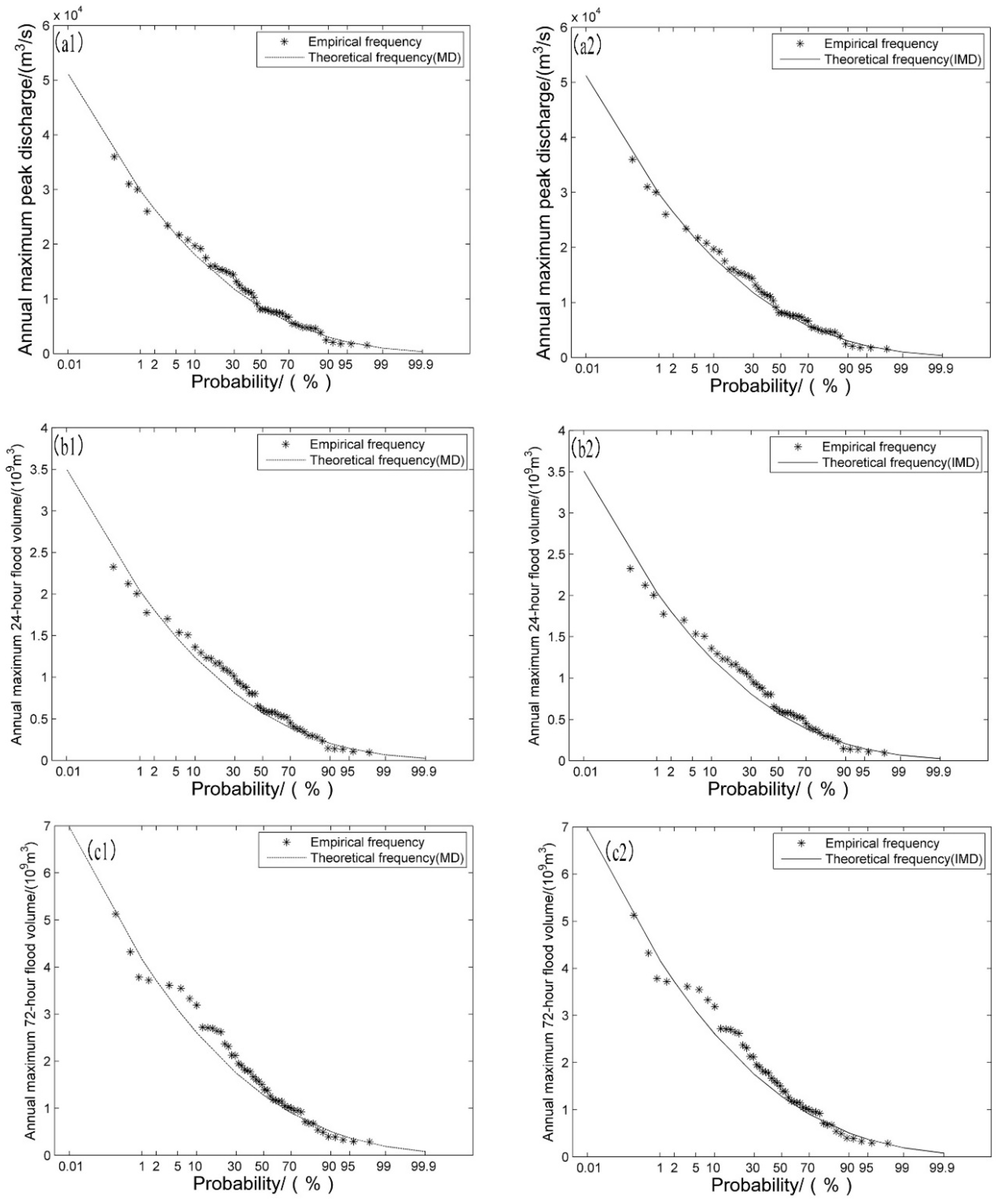
The D values for AMPDS, 24-h AMFVS and 72-h AMFVS are all less than the critical value $D_n(\alpha )$, which is equal to 0.194 at the 5% significance level. This result means that the P3, MD and IMD methods provide a satisfactory fit. The results show that P3 provides the best fit of the three methods. However, regarding the mechanism, the use of P3 distribution fitting is based on satisfying the stationarity hypothesis; in fact, the observed data of the Ankang hydrological station are consistent with the non-stationarity phenomenon. Thus, it is not reasonable to use the P3 distribution after environmental change. Meanwhile, it can also be seen that the AIC criterion values of the IMD method for the three flood characteristic series are all less than the corresponding criterion values of the MD method, which indicates that the IMD method is better. This result proved that our method improved the mechanism of mixed distribution and that our work is meaningful. The fitting results of the MD and IMD methods are given in Figure 7.

As is shown in

Table 13. Design flood results of each flood characteristic series with the MD and IMD methods.

Flood Characteristic Series		Return Periods in Years
		10,000	5000	1000	500	300	200	100	20	5
AMPDS (m3/s)	1999 design report	48,100	45,500	39,300	36,700	34,600	32,800	30,000	23,000	16,100
	P3	48,640	45,802	39,106	36,165	33,971	32,210	29,152	21,730	14,662
	MD	51,161	48,026	40,652	37,425	35,022	33,097	29,764	21,730	14,193
	IMD *	51,174	48,037	40,659	37,430	35,025	33,099	29,764	21,726	14,187
	Difference (1) (%)	6.39	5.58	3.46	1.99	1.23	0.91	−0.79	−5.54	−11.88
	Difference (2) (%)	5.21	4.88	3.97	3.50	3.10	2.76	2.10	−0.02	−3.24
	Difference (3) (%)	0.026	0.023	0.016	0.012	0.009	0.006	0.000	−0.018	−0.047
24-h AMFVS (108 m3)	P3	32.978	31.108	26.689	24.745	23.293	22.125	20.096	15.151	10.402
	MD	35.005	32.858	27.809	25.599	23.954	22.636	20.353	14.854	9.696
	IMD *	35.051	32.902	27.845	25.633	23.985	22.665	20.380	14.873	9.709
	Difference (2) (%)	6.29	5.77	4.33	3.59	2.97	2.44	1.41	−1.84	−6.67
	Difference (3) (%)	0.1310	0.1310	0.1309	0.1309	0.1308	0.1308	0.1308	0.1306	0.1306
72-h AMFVS (108 m3)	P3	65.067	61.568	53.278	49.617	46.876	44.669	40.824	31.385	22.191
	MD	69.726	65.629	55.969	51.729	48.565	46.027	41.622	30.939	20.786
	IMD *	69.743	65.645	55.981	51.739	48.574	46.035	41.629	30.942	20.785
	Difference (2) (%)	7.19	6.62	5.07	4.28	3.62	3.06	1.97	−1.41	−6.34
	Difference (3) (%)	0.024	0.023	0.021	0.020	0.019	0.018	0.016	0.009	−0.001

* represents the best fitness MD methods. Difference (1) represents the difference percentage in the best fitness MD methods compared with 1999 design report results, difference (2) represents the difference percentage in the best fitness MD methods compared with P3 and difference (3) represents the difference percentage in IMD compared with MD.

, for AMPDS, the differences in the design flood values between the best fitness MD methods and the 1999 design flood results are larger at high return periods and smaller at low return periods, with a difference of −11.88%~6.39%. The design flood value between the best fitness MD methods and the P3 results, without considering the non-stationarity data, has the same changing trends. The differences of AMPDS, 24-h AMFVS and 72-h AMFVS are −3.24%~5.21%, −6.67%~6.29% and −6.34%~7.19%, respectively. From Table 13, we can also see that the design value calculated by the IMD method of the flood series is slightly increased compared with the MD method. However, the IMD method may cause larger changes in the design flood values in other basins.

Tang et al. [54] developed the historical extraordinary flood-concerned mixed-distribution method (HFCMM) to overcome the shortcomings of the traditional methods without considering historical extraordinary flood events. However, their study focused on comparing the modelling results of different probability distribution function tail types rather than the difference in the design flood values.

Zeng et al. [18] used MD to estimate the design flood values of the Xidayang reservoir, which is located in the Daqinghe River Basin, in the northern part of China. All the design values decreased by 0.03%–20.24% with different return periods compared with the P3 distribution. However, both design flood values estimated by MD or IMD in our study increased for high return periods but decreased for small return periods. The cause of this phenomenon may be that our study area and the study area of Zeng are located in different river basins and different parts of China. Different factors such as different changes in land use cause different mechanisms of runoff generation and convergence in different basins. Thus, the design flood results we obtained are also reasonable. Yan et al. [22] noted that the time-varying two-component mixture distribution (TTMD) models exhibited better fitting results than and outperformed the stationary models in both the Huanxian and Xianyang stations of the Weihe River Basin. We can also develop the time-varying improved mixed distribution to consider the time variations of the parameters in future work.

5. Conclusions

Taking the Ankang hydrological station in the upper reaches of the Hanjiang River Basin as the research area, the trend and change point of the flood characteristic series were studied by the hydrological variation diagnosis system. The difference in the design flood values under four conditions showed the large significance of the non-stationary flood frequency analysis and the historical extraordinary flood data. The proposed IMD method was based on a mixed distribution and the calculation principle of discontinuous samples. The genetic algorithm was employed to estimate the parameters. The main conclusions of this paper were drawn as follows.

(1)

Hydrological series diagnosis was performed by using a variant diagnostic system. The trends of AMPDS, 24-h AMFVS and 72-h AMFVS at the Ankang hydrological station all decreased significantly at the 5% significance level. However, the final variant form was the change point, which illustrated that the change points of all flood characteristic series were in the year of 1987. This result was mainly related to the construction of the Ankang reservoir.

(2)

Based on the principle of MD, we proposed the methods of IMD, for which the genetic algorithm was applied, to estimate the parameters and the information of historical extraordinary floods was supplemented in the series after the change point. Meanwhile, the superiority of IMD was demonstrated by the consideration of both environment changes and historical extraordinary floods. Although the design flood of IMD was slightly larger than MD at the Ankang hydrological station, adding historical extraordinary flood data into both sub-series divided by the change point improved the theoretical mechanism of the mixed distribution. The new design flood based on IMD provides the basis for the regulation of reservoir floods in the upper reaches of the Hanjiang River.

Compared with other research of mixed distribution, the greatest advantage of this study is that the discontinuity and non-stationarity of flood samples are solved simultaneously. Taking historical extraordinary floods into sub-series both before and after the change point improved the physical mechanism of mixed distribution under a changing environment.

References

- Stocker, T.F.; Qin, D.; Plattner, G.-K.; Tignor, M.M.B.; Allen, S.K.; Boschung, J.; Nauels, A.; Xia, Y.; Bex, V.; Midgley, P.M. Climate Change 2013 the Physical Science Basis: Working Group I Contribution to the Fifth Assessment Report of the Intergovernmental Panel on Climate Change; Cambridge University Press: Cambridge, UK; New York, NY, USA, 2013; pp. 1–1535, ISBN 978-1-107-66182-0 Paperback, ISBN 978-1-107-05799-9 Hardback. [Google Scholar]
- Zhang, S.L.; Yang, D.W.; Yang, H.B.; Lei, H.M. Analysis of the dominant causes for runoff reduction in five major basins over China during 1960–2010. Adv. Water Sci. 2015, 26, 605–613. [Google Scholar]
- Milly, P.C.D.; Betancourt, J.; Falkenmark, M.; Hirsch, R.M.; Kundzewicz, Z.W.; Lettenmaier, D.P.; Stouffer, R.J. Climate change-Stationarity is dead: Whither water management? Science 2009, 319, 573–574. [Google Scholar] [CrossRef] [PubMed]
- Liang, Z.M.; Hu, Y.M.; Wang, J. Advances in hydrological frequency analysis of non-stationary time series. Adv. Water Sci. 2011, 22, 864–871. [Google Scholar]
- Labat, D.; Ababou, R.; Mangin, A. Rainfall-runoff relations for karstic springs. Part II: Continuous wavelet and discrete orthogonal multiresolution analyses. J. Hydrol. 2000, 238, 149–178. [Google Scholar] [CrossRef]
- Seidou, O.; Ramsay, A.; Nistor, I. Climate change impacts on extreme floods I: Combining imperfect deterministic simulations and non-stationary frequency analysis. Nat. Hazards 2012, 61, 647–659. [Google Scholar] [CrossRef]
- Hu, Y.M.; Liang, Z.M.; Jiang, X.L.; Bu, H. Non-stationary hydrological frequency analysis based on the reconstruction of extreme hydrological series. In Proceedings of the International Association of Hydrological Sciences, Prague, Czech Republic, 22 June–2 July 2015. [Google Scholar]
- Saifulllah, M.; Li, Z.J.; Li, Q.L.; Hashim, S.; Zaman, M.; Liu, K.L. Assessment the impacts of land surface change on the hydrological process based on similar hydro-meteorological conditions with swat. Fresenius Environ. Bull. 2016, 25, 3071–3082. [Google Scholar]
- Strupczewski, W.G.; Singh, V.P.; Feluch, W. Non-stationary approach to at-site flood frequency modeling I. Maximum likelihood estimation. J. Hydrol. 2001, 248, 123–142. [Google Scholar] [CrossRef]
- Strupczewski, W.G.; Kaczmarek, Z. Non-stationary approach to at-site flood frequency modeling II. Weighted least squares estimation. J. Hydrol. 2001, 248, 143–151. [Google Scholar] [CrossRef]
- Strupczewski, W.G.; Singh, V.P.; Mitosek, H.T. Non-stationary approach to at-site flood frequency modeling III. Flood analysis of Polish rivers. J. Hydrol. 2001, 248, 152–167. [Google Scholar] [CrossRef]
- Singh, V.P.; Wang, S.X.; Zhang, L. Frequency analysis of nonidentically distributed hydrologic flood data. J. Hydrol. 2005, 307, 175–195. [Google Scholar] [CrossRef]
- Singh, K.P.; Sinclair, R.A. Two-distribution method for flood frequency analysis ASCE. J. Hydraul. Div. 1972, 98, 28–44. [Google Scholar]
- Alila, Y.; Mtiraoui, A. Implications of heterogeneous flood-frequency distributions on traditional stream-discharge prediction techniques. Hydrol. Process. 2002, 16, 1065–1084. [Google Scholar] [CrossRef]
- Waylen, P.; Woo, M. Prediction of annual floods generated by mixed processes. Water Resour. Res. 1982, 18, 1283–1286. [Google Scholar] [CrossRef]
- Fischer, S.; Schumann, A.; Schulte, M. Characterisation of seasonal flood types according to timescales in mixed probability distributions. J. Hydrol. 2016, 539, 38–56. [Google Scholar] [CrossRef]
- Sivapalan, M.; Bloschl, G.; Merz, R.; Gutknecht, D. Linking flood frequency to long-term water balance: Incorporating effects of seasonality. Water Resour. Res. 2005, 41, 303–315. [Google Scholar] [CrossRef]
- Zeng, H.; Feng, P.; Li, X. Reservoir flood routing considering the non-stationarity of flood series in north China. Water Resour. Manag. 2014, 28, 4273–4287. [Google Scholar] [CrossRef]
- Rossi, F.; Fiorentino, M.; Versace, P. Two-component extreme value distribution for flood frequency analysis. Water Resour. Res. 1984, 20, 847–856. [Google Scholar] [CrossRef]
- Fiorentino, M.; Arora, K.; Singh, V.P. The two-component extreme value distribution for flood frequency analysis: Derivation of a new estimation method. Stoch. Hydrol. Hydraul. 1987, 1, 199–208. [Google Scholar] [CrossRef]
- Grego, J.M.; Yates, P.A. Point and standard error estimation for quantiles of mixed flood distributions. J. Hydrol. 2010, 391, 289–301. [Google Scholar] [CrossRef]
- Yan, L.; Xiong, L.H.; Liu, D.D.; Hu, T.S.; Xu, C.Y. Frequency analysis of nonstationary annual maximum flood series using the time-varying two-component mixture distributions. Hydrol. Process. 2017, 31, 69–89. [Google Scholar] [CrossRef]
- Schendel, T.; Thongwichian, R. Considering historical flood events in flood frequency analysis: Is it worth the effort? Adv. Water Resour. 2017, 105, 144–153. [Google Scholar] [CrossRef]
- Strupczewski, W.G.; Kochanek, K.; Bogdanowicz, E. Historical floods in flood frequency analysis: Is this game worth the candle? J. Hydrol. 2017, 554, 800–816. [Google Scholar] [CrossRef]
- Benito, G.; Lang, M.; Barriendos, M.; Llasat, C.M.; Frances, F.; Ouarda, T.; Thorndycraft, V.R.; Enzel, Y.; Bardossy, A.; Coeur, D.; et al. Use of Systematic, Palaeoflood and Historical Data for the Improvement of Flood Risk Estimation. Review of Scientific Methods. Nat. Hazards 2004, 31, 623–643. [Google Scholar]
- Parent, E.; Bernier, J. Bayesian POT modeling for historical data. J. Hydrol. 2003, 274, 95–108. [Google Scholar] [CrossRef]
- Halbert, K.; Nguyen, C.C.; Payrastre, O.; Gaume, E. Reducing uncertainty in flood frequency analyses: A comparison of local and regional approaches involving information on extreme historical floods. J. Hydrol. 2016, 541, 90–98. [Google Scholar] [CrossRef]
- Reis, D.S.; Stedinger, J.R. Bayesian MCMC flood frequency analysis with historical information. J. Hydrol. 2005, 313, 97–116. [Google Scholar] [CrossRef]
- Ding, J.; Yang, R. The determination of probability weighted moments with the incorporation of extraordinary values into sample data and their application to estimating parameters for the Pearson type three distribution. J. Hydrol. 1988, 101, 63–81. [Google Scholar]
- Frances, F.; Salas, J.D.; Boes, D.C. Flood frequency analysis with systematic and historical or paleoflood data based on the two-parameter general extreme value models. Water Resour. Res. 1994, 30, 1653–1664. [Google Scholar] [CrossRef]
- Machado, M.J.; Botero, B.A.; Lopez, J.; Frances, F.; Diez-Herrero, A.; Benito, G. Flood frequency analysis of historical flood data under stationary and non-stationary modelling. Hydrol. Earth Syst. Sci. 2015, 19, 2561–2576. [Google Scholar] [CrossRef] [Green Version]
- Xie, P.; Cheng, G.C.; Lei, H.F.; Wu, F.Y. Hydrological alteration diagnosis system. J. Hydroelectr. Eng. 2010, 29, 85–91. [Google Scholar]
- Hurst, H.E. Long-term storage capacity of reservoirs. Trans. Am. Soc. Civ. Eng. 1951, 116, 776–808. [Google Scholar]
- Gautheir, T.D. Detecting trends using spearman’s rank correlation coefficient. Environ. Forensics 2001, 2, 359–362. [Google Scholar] [CrossRef]
- Tabari, H.; Aghajanloo, M.B. Temporal pattern of aridity index in Iran with considering precipitation and evapotranspiration trends. Int. J. Climatol. 2013, 33, 396–409. [Google Scholar] [CrossRef]
- Lee, A.F.S.; Heghinian, S.M. A shift of the mean level in a sequence of independent normal random variables: A bayesian approach. Technometrics 1977, 19, 503–506. [Google Scholar] [CrossRef]
- Zhang, Q.; Gu, X.H.; Singh, V.P.; Xiao, M.Z. Flood frequency analysis with consideration of hydrological alterations: Changing properties, causes and implications. J. Hydrol. 2014, 519, 803–813. [Google Scholar] [CrossRef]
- Pettitt, A.N. Some Results on Estimating a Change-Point Using Non-Parametric Type Statistics. J. Stat. Comput. Simul. 1980, 11, 261–272. [Google Scholar] [CrossRef]
- Mann, H.B. Nonparametric tests against trend: 1. Introd. Econ. 1945, 13, 245–259. [Google Scholar] [CrossRef]
- Kendall, M. Rank Correlation Methods, 4th ed.; Charles Griffin: London, UK, 1975. [Google Scholar]
- Strupczewski, W.G.; Kochanek, K.; Bogdanowicz, E.; Markiewicz, I. On seasonal approach to flood frequency modelling. Part I: Two-component distribution revisited. Hydrol. Process. 2012, 26, 705–716. [Google Scholar] [CrossRef]
- Kochanek, K.; Strupczewski, W.G.; Bogdanowicz, E. On seasonal approach to flood frequency modelling. Part II: Flood frequency analysis of Polish rivers. Hydrol. Process. 2012, 26, 717–730. [Google Scholar] [CrossRef]
- Ministry of Water Resources (MWR). Guidelines for Calculating Design Flood of Water Resources and Hydropower Projects; Chinese Water Resources and Hydropower Press: Beijing, China, 2006.
- Zhao, B.K.; Wang, L.P.; Li, J.Q.; Zhang, Y.K.; Yu, S. Study on computer curve fitting method for Pearson type-Ⅲ curve with discontinuous series. Water Resour. Power 2012, 30, 64–67. [Google Scholar]
- Chakravarti, I.M.; Laha, R.G.; Roy, J.D. Handbook of Methods of Applied Statistics. Vol. I: Techniques of Computation, Descriptive Methods, and Statistical Inference; John Wiley and Sons: New York, USA, 1967. [Google Scholar]
- Akaike, H. A new look at the statistical model identification. IEEE Trans. Autom. Control. 1974, 19, 716–723. [Google Scholar] [CrossRef]
- Hassanzadeh, Y.; Abdi, A.; Talatahari, S.; Singh, V.P. Meta-Heuristic Algorithms for Hydrologic Frequency Analysis. Water Resour. Manag. 2011, 25, 1855–1879. [Google Scholar] [CrossRef]
- Dai, Q.; Han, D.; Rico-Ramirez, M.A.; Zhuo, L.; Nanding, N.; Islam, T. Radar rainfall uncertainty modelling influenced by wind. Hydrol. Process. 2015, 29, 1704–1716. [Google Scholar] [CrossRef]
- Lee, T.; Jeong, C. Frequency Analysis of Nonidentically Distributed Hydrometeorological Extremes Associated with Large-Scale Climate Variability Applied to South Korea. J. Appl. Meteorol. Climatol. 2014, 53, 1193–1212. [Google Scholar] [CrossRef]
- Ministry of Water Resources of People’s Republic of China. Design Criterion of Reservoir Management; China Water Resources and Hydropower Press: Beijing, China, 1996.
- Yang, Z.L. Analysis of design flood in Ankang Hydropower Station. Water Power 1990, 11, 21–25. [Google Scholar]
- Yang, Z.L. Rechecking of flood discharge data in Ankang hydrology station. Hydrology 1984, 4, 29–36. [Google Scholar]
- Xiong, L.H.; Jiang, C.; Xu, C.Y.; Yu, K.X.; Guo, S.L. A framework of change-point detection for multivariate hydrological series. Water Resour. Res. 2015, 51, 8198–8217. [Google Scholar] [CrossRef]
- Tang, Y.H.; Chen, X.H.; Ye, C.Q.; Zhang, J.M.; Zhang, L.J. Application of historical flood-concerned mixed distribution with different tail types of PDFs. J. Hydroelectr. Eng. 2015, 34, 31–37. [Google Scholar]
Figure 1.
Map of the upper Hanjiang Basin above the Ankang hydrological station.
Figure 2.
The hydrograph of the 1974 typical flood and the 1983 largest flood. (a) The hydrograph of the typical flood in 1974; and (b) The hydrograph of the largest flood in 1983.
Figure 3.
Correlation relationship between the flood peak and volume at the Ankang hydrological station.
Figure 4.
Variation between the design flood value of annual maximum peak discharge series (AMPDS) simulated by Monte Carlo and estimated by genetic algorithm (GA). (a) Design flood values of AMPDS simulated by Monte Carlo and estimated by GA at different return periods; and (b) Quantile-Quantile plots between design flood values of AMPDS simulated by Monte Carlo and estimated by GA.
Figure 5.
95% confidence intervals computed using the bootstrap method for flood characteristic series. (a) 95% confidence intervals of the annual maximum peak discharge; (b) 95% confidence intervals of the annual maximum 24-h flood volume; and (c) 95% confidence intervals of the annual maximum 72-h flood volume.
Figure 6.
Fitting results for each flood characteristic series under four conditions. (a) Fitting results of the annual maximum peak discharge; (b) Fitting results of the annual maximum 24-h flood volume; and (c) Fitting results of the annual maximum 72-h flood volume.
Figure 7.
Fitting results of the MD and IMD methods. (a1) MD fitting results of AMPDS; (a2) IMD fitting results of AMPDS; (b1) MD fitting results of annual maximum 24-h flood volume series (24-h AMFVS); (b2) IMD fitting results of 24-h AMFVS; (c1) MD fitting results of 72-h AMFVS; and (c2) IMD fitting results of 72-h AMFVS.