Temporal and Spatial Flow Variations over a Movable Scour Hole Downstream of a Grade-Control Structure with a PIV System

Abstract

Weirs or grade-control structures (GCSs) are frequently adopted to protect bridges or control riverbed degradation. Scour holes may develop downstream of these hydraulic structures. Laboratory experiments have been performed in this study, using sophisticated equipment and newly developed procedures. The purpose was to investigate important characteristics of the turbulent flow in the movable scour hole. The results of these experiments demonstrated the significance of instantaneous shear stress in the scouring process. The measured Reynolds stress can be fitted with the theoretical equation reasonably well. Furthermore, the results revealed that the normalized mean vertical velocity profiles in the diffusion region of the scour hole can be fitted with a Gaussian curve. An analysis of the turbulence intensity measurements showed that the turbulent flow is anisotropic in the scour hole. The turbulence intensities also decreased with time as the scour hole gradually approached equilibrium.

1. Introduction

Many rivers in Taiwan have steep slopes and rapid flows. The flow stage often varies rapidly during typhoon seasons. This can cause severe degradation to the riverbed and levee foundation, and also bridge pile exposures. A grade-control structures (GCS) is frequently adopted to reduce riverbed degradation. For steep rivers, several consecutive low-head GCSs are used. The top of the GCS is flush with the channel bed to reduce possible downstream local scour if required.

Lu et al. [1] conducted a literature review on several studies, including Schoklitsch [2], Bormann and Julien [3], Hoffmans and Verheij [4], Gaudio et al. [5], Gaudio and Marion [6], Lenzi et al. [7,8,9], Marion et al. [10,11], Pagliara [12], and Tregnaghi et al. [13,14], that investigated a scour situated downstream of a GCS or drop. The investigation included the equilibrium maximum scour depth and profiles. Gaudio et al. [5] further noted that scour profiles at equilibrium are affine.

Wu and Rajaratnam [15] divided the submerged flow into two broad classes: Impinging jet and surface flow regimes. The latter includes the breaking wave (or surface jump), surface wave, and surface jet. The boundaries of the two regimes were based on the change in direction of the tailwater. On the basis of the experimental data from the literature and also new data (Guan et al. [16]), Guan et al. [17] developed a new transition regime boundary equation as a function of the upstream Froude number and the ratio of the weir height to the tailwater depth.

Lu et al. [1] conducted laboratory experiments with dual GCSs and both steady and unsteady conditions. The first and the second scour holes were under clear-water and live-bed conditions, respectively. It was discovered that three distinct phases can be identified for the evolution of a scour hole downstream of a GCS. These are the initial, developing, and equilibrium phases. A scour evolution simulation scheme was also proposed. The proposed scheme can reasonably well predict the temporal variations of maximum scour depth for unsteady flows with both single and multiple peaks. However, detailed measurements of the turbulent flows were not performed. Guan et al. [18] performed a laboratory study to investigate the flow patterns and turbulence structures in a scour hole downstream of a submerged weir. The study was under conditions of low aspect ratios (less than about 3) and relatively flat slope gradients. The study aims to investigate the temporal and spatial variations of the flow in the scour hole downstream of a GCS for a wide, sloped channel. A sophisticated PIV (particle image velocimetry) system is used to further clarify the scouring phenomenon. The two-dimensional wide channel (high aspect ratio) was selected, as it is closer to the conditions for most of the natural rivers and reduces the flow measuring cost.

2. Experimental Set-Up and Procedure

2.1. Experimental Design and Flume

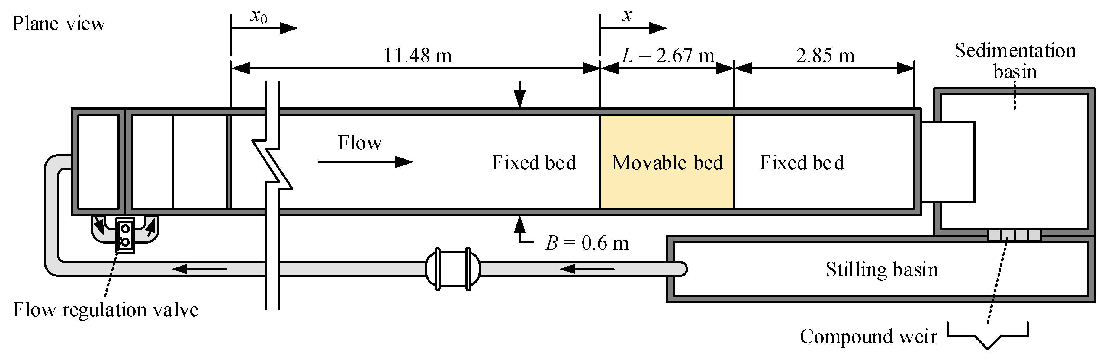
The experiments were performed in a 17.5 m long, 0.6 m wide, and 0.6 m deep laboratory flume with glass sidewalls (Figure 1). Two horizontal wooden plates with lengths of 11.48 m and 2.85 m were placed upstream and downstream of the sediment recess. A vertical wooden plate was also installed at the upstream end of the sediment recess to represent a GCS. The top of the GCS was flush with the surface of the movable bed. The working length of the flume L which represented the sediment recess was 2.67 m, selected to sufficiently guarantee full scour development without any geometrical interference. In this study, uniform gravel with a median size ($D_{50}$) of 2.7 mm and a geometric standard deviation (${\sigma }_g=\sqrt{D_{84}/D_{16}}$) of 1.4 was used. In general, ripple is not expected in a laboratory flume with a gravel bed (Gaudio et al. [19] and Ferraro et al. [20]). The clear-water condition (no upstream sediment supply) was considered to slightly simplify the experiments.

Table 1. Summary of the experimental conditions.

Run	${\mathit{S}}_{\mathit{b}}$	${\mathit{h}}_0$	$\mathit{q}$	${\mathit{U}}_0$	${\mathit{U}}_{\ast }$	${\mathbf{F}}_{\mathbf{r}}$	${\mathbf{R}}_{\mathbf{e}}$	$\mathit{B}/{\mathit{h}}_0$	${\mathit{d}}_{\mathbf{m},\mathbf{e}}$	${\mathit{x}}_{\mathbf{m},\mathbf{e}}$	${\mathit{l}}_{\mathbf{m},\mathbf{e}}$
		(m)	(m2/s)	(m/s)	(m/s)				(m)	(m)	(m)
M-1	0.01	0.017	0.0167	0.98	0.0397	2.41	15,757	35	0.049	0.18	0.56
M-2	0.01	0.025	0.0283	1.13	0.0476	2.29	26,045	24	0.066	0.25	0.98
S-1	0.015	0.016	0.0167	1.04	0.0473	2.63	17,327	38	0.082	0.19	0.70
S-2	0.015	0.023	0.0283	1.23	0.0561	2.59	26,206	26	0.118	0.23	1.03

Note: $S_b$ = bed slope; $h_0$ = average approach flow depth; $q$ = unit flow discharge; $U_0$ = average approach flow velocity; $U_{\ast }$ = average approach flow shear velocity; ${\mathrm{F}}_{\mathrm{r}}$ = Froude number; ${\mathrm{R}}_{\mathrm{e}}$ = Reynolds number; $B/h_0$ = aspect ratio; $d_{\mathrm{m},\mathrm{e}}$ = maximum scour depth at the equilibrium stage; $x_{\mathrm{m},\mathrm{e}}$ = position of maximum scour depth; $l_{\mathrm{m},\mathrm{e}}$ = maximum scour hole length at the equilibrium stage.

summarizes the experimental conditions. The water level measurements were conducted by using an ultrasonic transducer Keyence, Osaka, Japan, with a resolution ± 1 mm.

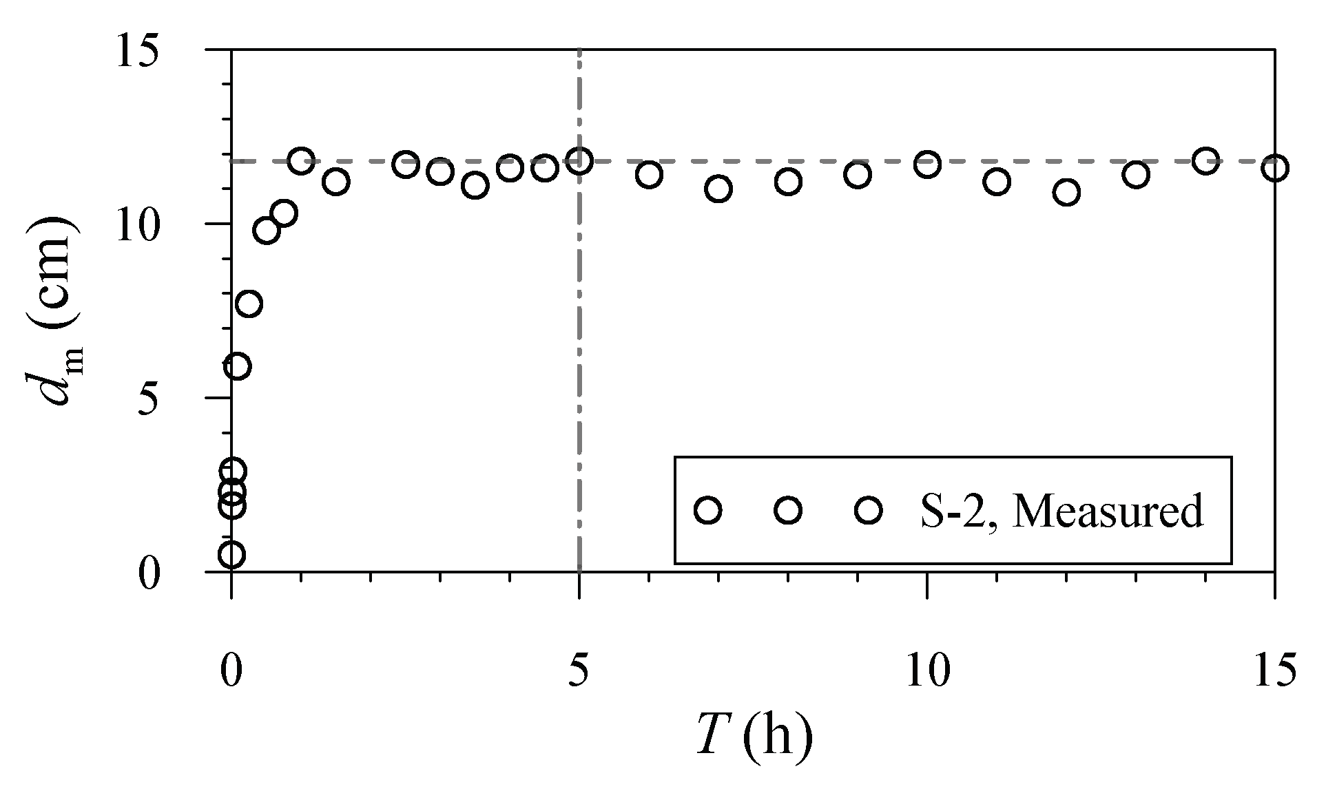
The experiments were conducted with two independent variables: Unit flow discharge $q$ and bed slope $S_b$. The flow discharges were selected on the basis of Froude law, with a length ratio ($L_r$) of 1/50 for the 5-year and 20-year flows of the Tou-Chien River, Hsin-Chu County, Taiwan. The slope range of 1–1.5% was typical for gravel bed rivers in Taiwan. The average approach flow depth $h_0$ was measured at $x_0$ = 8.48 m, where the flow was fully developed. The low relative submergences ($h_0/D_{50}$, ranged from 6 to 9) were mostly due to the gradients of steep slopes. Powell [21] reviewed the studies of Bathurst et al. [22] and Lawrence [23] on the effect of relative submergence. Figure 2 shows the evolution of maximum scour depth ($d_{\mathrm{m}}$) for a preliminary test (Run S-2). The result indicated a very high scouring rate for the first hour, and the scouring phenomenon almost reached equilibrium after 5 h. The turbidity of the flow was extremely high for the first 15 min. Thus, tests were conducted at 15 min, 1 h, and 5 h. The experimental duration of 5 h in this study represents the peak flow duration for an unsteady flood event.

The Froude number ${\mathrm{F}}_{\mathrm{r}}$ ranged from 2.29–2.63 (supercritical flows, ${\mathrm{F}}_{\mathrm{r}}=U_0/\sqrt{g{h}_0}$) and the aspect ratio ranged from 24–38. The aspect ratios ($B/h_0$) were greater than 10, making it reasonable to assume that the resistance of the side walls was negligible and the flows were two-dimensional (2-D). As a result, a two-dimensional measuring system was adopted in the current study.

2.2. PIV Measuring System

The images analyzed were captured using a high-resolution digital camera (Phantom Miro ex4) with a resolution of $800\times 600$ pixels and highest frequency array 1265 Hz. In the conventional PIV measurement, lasers are predominantly adopted in PIV setups. The conventional methods are difficult to apply in our movable bed experiments due to the scattering of particles.

To reduce the particle scattering and produce reasonably uniform light, a sheet of soft light paper was attached on the back sidewall and halogen lamps were adopted in this study. Black Acrylonitrile–Butadiene–Styrene (ABS) particles were used as the seeding particles. The particle size ranged from 0.25–0.3 mm and the density was 1.04 g/cm³. The image velocimetry was then adopted to analyze the moving trajectories of the black particles projected on the soft light paper.

3. Results and Discussion

3.1. Verification of the PIV Measuring System

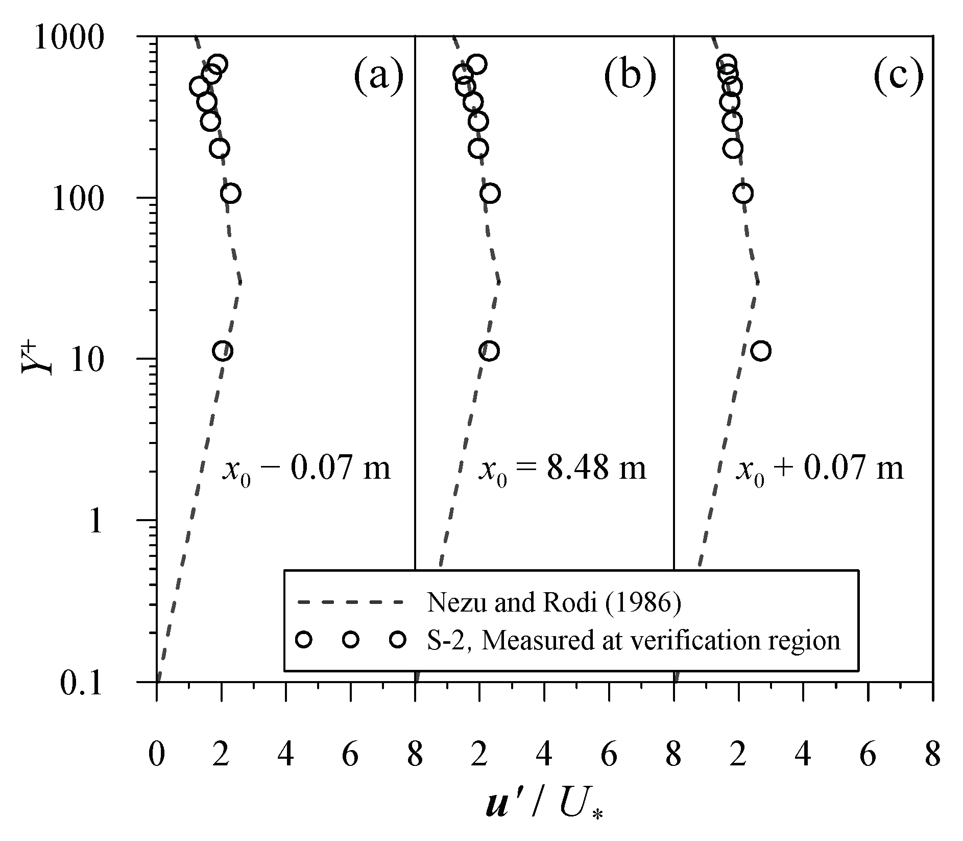
A preliminary test was performed in the fully developed zone of the channel to compare the results of the PIV measuring system with those of Nezu and Rodi’s [24] empirical formula, which had been verified with 2-D fiber-optic laser doppler velocimetry (Lu et al. [25]). Figure 3 shows three measured dimensionless longitudinal turbulence intensity profiles in the fully developed verification region (center located at $x_0$ = 8.48 m) with Nezu and Rodi’s [24] empirical curves, in which $Y^{+}=U_{\ast }{y}_i\rho /\mu$ and $y_i$ is the elevation from the fixed channel bed, $\rho$ is the water density, $\mu$ is the dynamic viscosity of water, and $\mathit{u}\prime =\sqrt{\overline{u^{\prime 2}}}$ ($u$ = longitudinal fluctuating velocity). The grid size for the analysis of PIV data was 7 mm. The results indicate that generally the measured profiles are in good agreement with the curves presented by Nezu and Rodi [24], except for the region very close to the water surface. In this region, light may have been slightly affected by the outdoor environment. As our primary focus was on the flow field near the channel boundary (e.g., boundary shear stress), the error near the water surface was ignored.

3.2. Two-Dimensional Velocity Distribution

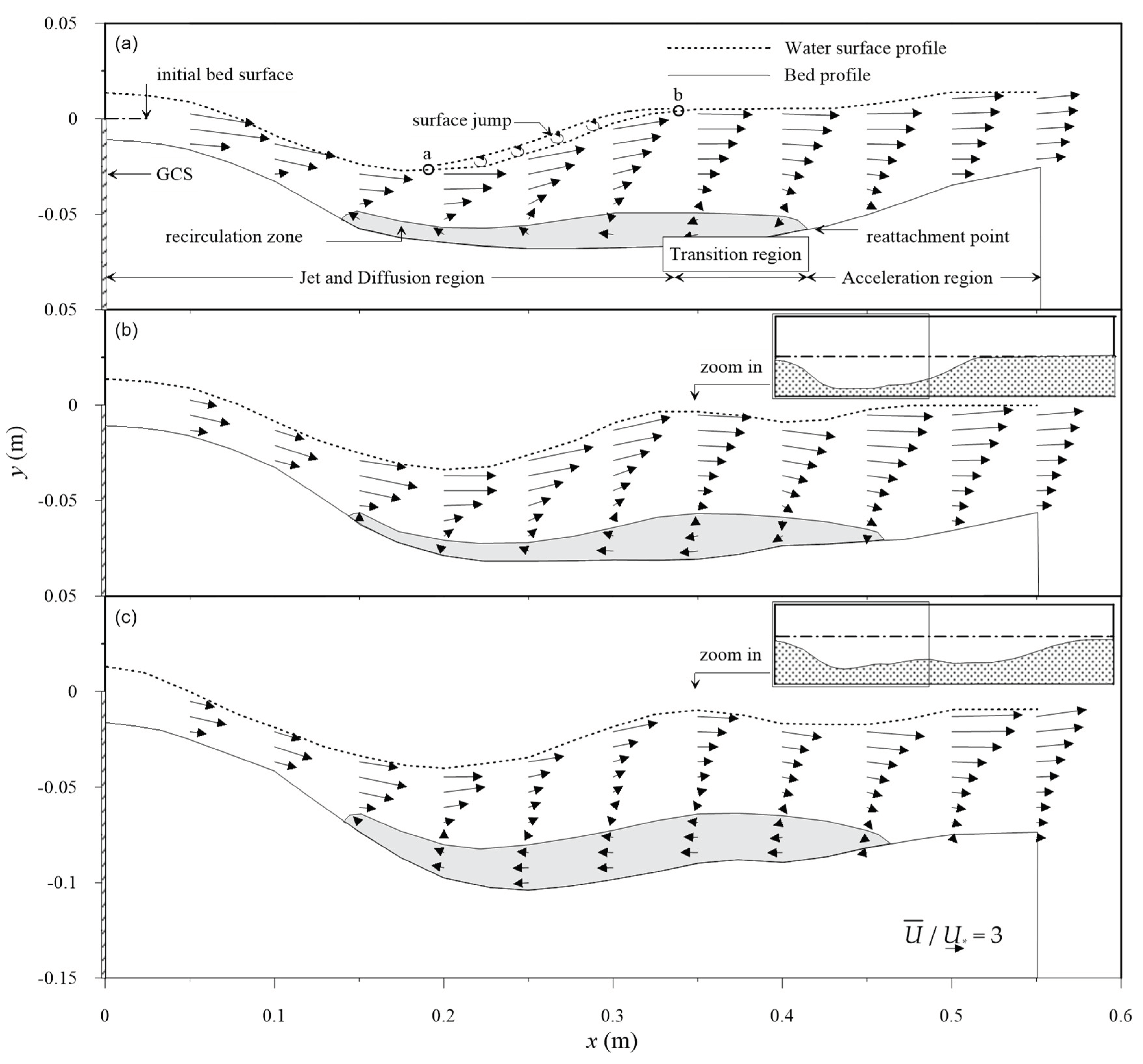
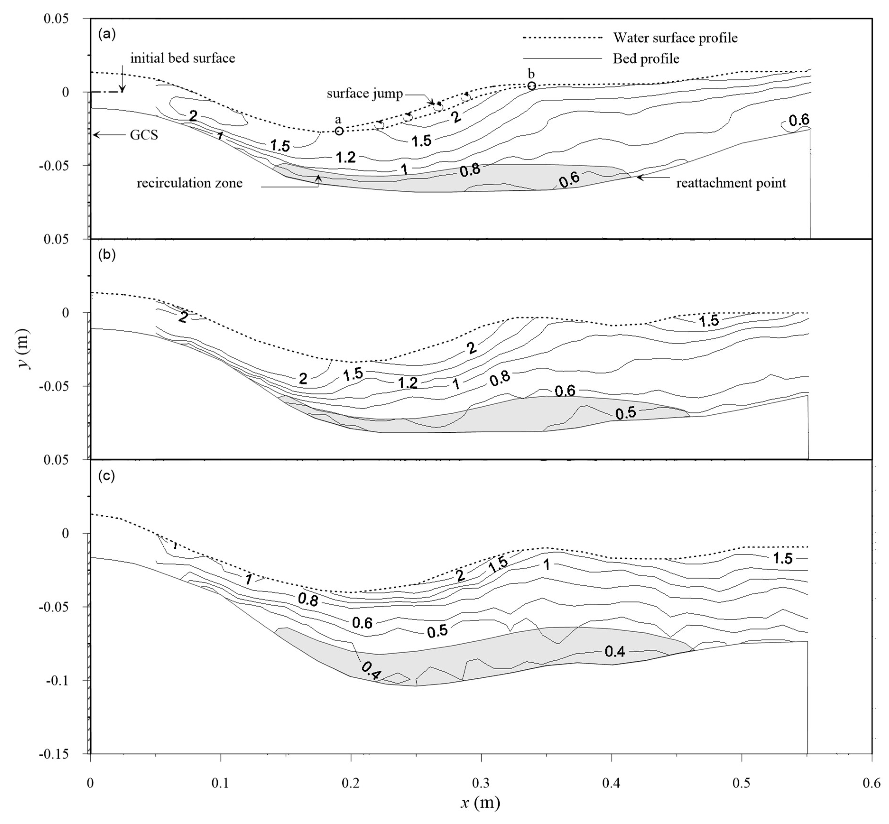
Analysis of the mean velocity profiles for the conditions investigated (Table 1) revealed that the flow in the scour hole can be qualitatively divided into three regions shown in Figure 4a: Jet and diffusion, transition, and acceleration regions (Run S-2, $S_b$ = 0.015, $q$ = 0.0283 m²/s, ${\mathrm{F}}_{\mathrm{r}}$ = 2.59). In Figure 4, $\overline{U}$ is the vectorial mean velocity. For the purpose of demonstration, Run S-2 was selected as a representative case as it has the highest flow intensity (high $q$ and $S_b$ values) and the largest scour hole.

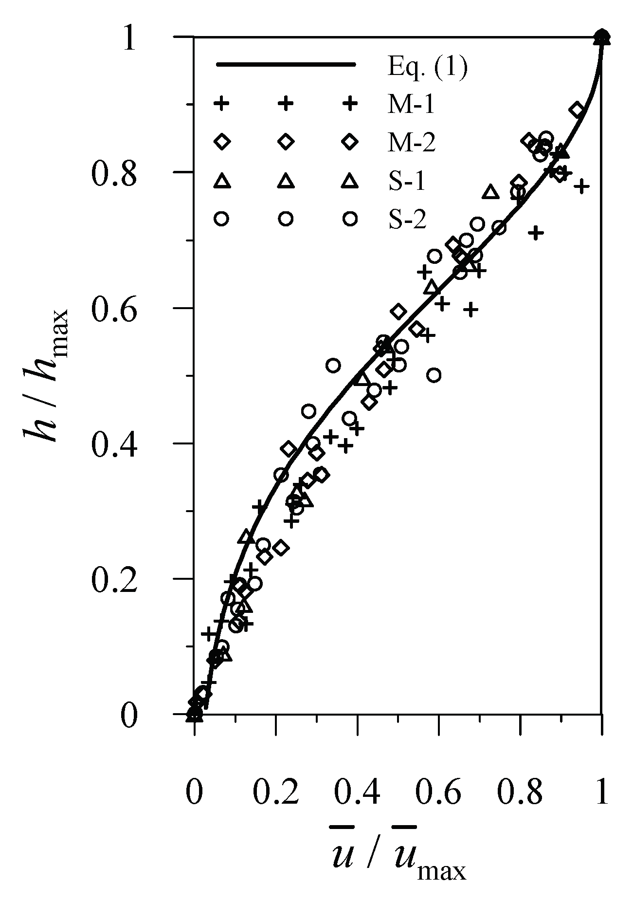
As the flow passes the submerged GCS, the supercritical high-velocity fluid behaves like a submerged jet, oscillating occasionally. When the jet deflection angle is large (the early stage of the scouring process), the impinging jet (Wu and Rajaratnam [15]) may occur. This may entrain a significant amount of bed sediment, causing a “bursting phenomenon” (Lu et al. [1]). A surface jump is usually formed slightly downstream. Severe mixing of turbulence and energy dissipation occur in the jump. Point b is the highest point of the surface jump, while point a is the lowest point of the water surface profile before the surface jump. As depicted in Figure 5, the normalized flow velocity profiles can be approximated as a normal distribution near zone ab, indicating the diffusion characteristic of the submerged jet. As a result, the first region from the entrance (GCS) to point b is defined as the jet and diffusion region. A recirculation zone is also formed when the scour hole is deep enough. The reattachment point downstream of the recirculation zone usually continues to move slowly downstream with time.

The normalized velocity profiles can be approximated as a normal distribution in zone ab above the recirculation zone:

$$\frac{\overline{u}}{{\overline{u}}_{\max }}=\exp \left(\frac{-h/h_{\max }}{2{\hat{\sigma }}_u{}^2}\right)$$

(1)

where $\overline{u}$, $h$, ${\overline{u}}_{\max }$ and $h_{\max }$ are the mean longitudinal velocity, vertical distance measured above the recirculation zone, maximum $\overline{u}$ value and $h$ value at ${\overline{u}}_{\max }$, respectively. The upper envelope curve of the recirculation zone in Figure 4 was obtained by interpolation. Based on the regression analysis, the standard deviation ${\hat{\sigma }}_u$ was 0.370. The result indicates that although the maximum velocity of the submerged jet decreases as the flow expands downstream, the similarity criterion can be applied to zone ab.

The last region within the scour hole is called acceleration region, occurring when the channel bed elevation increases rapidly near the downstream end of the scour hole. The flow accelerates due to the decrease of the flow depth, and gradually approaches the incoming flow condition. The region between the jet and diffusion region and the acceleration region is called transition region. This region elongates with time, and the elevation of the channel bottom flattens out (or only slightly increases) downstream, as shown in Figure 4c.

The maximum scour depth $d_{\mathrm{m},\mathrm{e}}$, position of maximum scour depth $x_{\mathrm{m},\mathrm{e}}$ and maximum scour hole length $l_{\mathrm{m},\mathrm{e}}$ at the equilibrium stage (5 h) are also summarized in Table 1. Figure 4c indicates that after the vertical evolution of the maximum scour depth (refer to Figure 2), the scour hole tends to gradually evolve in the downstream direction, revealing that the length of the sediment recess ($L$ in Figure 1) is long enough.

3.3. Turbulence Intensities

Figure 6 and Figure 7 show the dimensionless longitudinal and vertical turbulence intensity contours along the channel centerline, in which $\mathit{u}\prime =\sqrt{\overline{u^{\prime 2}}}$ ($u\prime$ = longitudinal fluctuating velocity), and $\mathit{v}\prime =\sqrt{\overline{v^{\prime 2}}}$ ($v\prime$ = vertical fluctuating velocity), and $U_{\ast }$ = approach flow shear velocity. The measuring frequency of the PIV system was 1/500 s. As shown in Table 1, all the Froude numbers of the approach flows are greater than 2 (supercritical flows). Figure 6 and Figure 7 reveal that high turbulence intensity values occur near the entrance region and zone ab (defined previously, see Figure 4a), where the surface jump occurs.

In general, the dimensionless longitudinal turbulence intensity is higher than the dimensionless vertical turbulence intensity, indicating the turbulent flow is anisotropic. The distributions of $\mathit{u}\prime /U_{\ast }$ and $\mathit{v}\prime /U_{\ast }$ are very similar, as there were two local maxima occurring at the entrance region and the surface jump. Regarding the jet and diffusion region ($x\approx$ 0.15–0.3 m), only the values near the scour hole bottom decrease for $T$ in the range of 15 min to 1 h. For $T$ in the range of 1 to 5 h, $\mathit{u}\prime /U_{\ast }$ decreases by approximately 25%, while $\mathit{v}\prime /U_{\ast }$ decreases by approximately 20%; and $\mathit{u}\prime /U_{\ast }\cong 1.5\mathit{v}\prime /U_{\ast }$ near the scour hole bottom. By contrast, $\mathit{u}\prime /U_{\ast }$ decreases by approximately 50% near the water surface, while $\mathit{v}\prime /U_{\ast }$ only decreases slightly, especially for the area near the surface jump. A knowledge of turbulent flow characteristics within the scour hole may help to improve the accuracy of the scour prediction models. For instance, Dodaro et al. [26] and Dodaro et al. [27] employed instantaneous flow velocity data to accurately predict scour evolution downstream of a rigid bed.

3.4. Reynolds Shear Stress

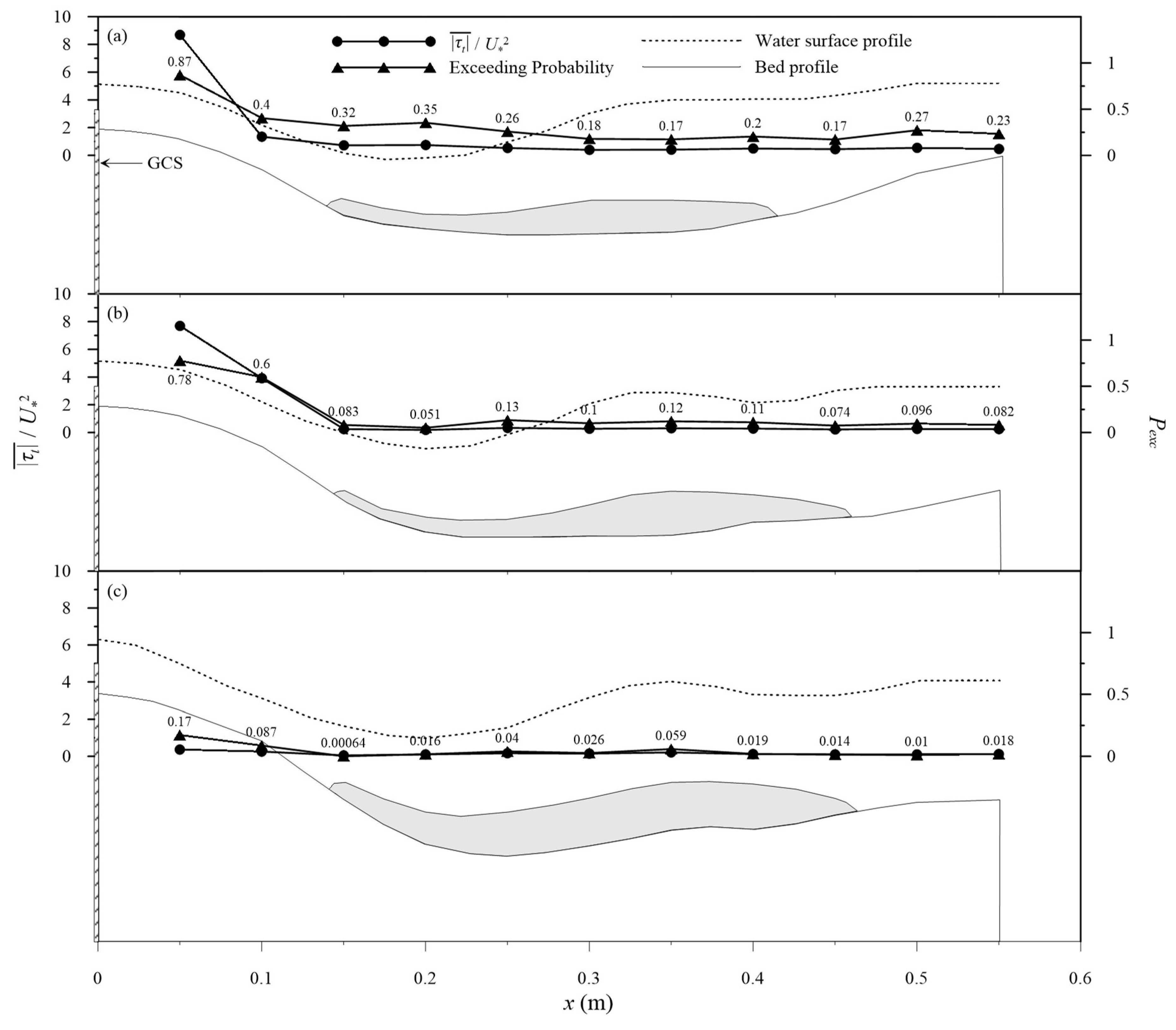
Figure 8 shows the variations in the dimensionless mean absolute Reynolds shear stress $\overline{\left|{\tau }_t\right|}/U_{\ast }{}^2$ and the exceeding probability $P_{exc}$ along the boundary of the scour hole with time. The exceeding probability is defined as

$$P_{exc}=N_{\left|{\tau }_t\right|>{\tau }_c}/N_{total},$$

(2)

where $N_{\left|{\tau }_t\right|>{\tau }_c}$ is the number of $\left|{\tau }_t\right|$ values greater than the critical shear stress ${\tau }_c$, and $N_{total}$ is the total number of the instantaneous Reynolds shear stress ${\tau }_t$ values collected during the sampling period (8 s). The Reynolds shear stress (${\tau }_t=-\rho \mathit{u}\prime \mathit{v}\prime$) was obtained based on the Shields diagram, and ${\tau }_c$ = 2.1 N/cm² for $D_{50}$ = 2.7 mm. With consideration of particle size roughness in the movable boundary ($D_{50}$ = 2.7 mm), a grid size of 7 mm was adopted in the analysis of PIV data. The lowest point selected for estimating the bed shear stress was therefore set at 3.5 mm above the bed.

Figure 8a shows that the dimensionless mean absolute Reynolds shear stress $\overline{\left|{\tau }_t\right|}/U_{\ast }{}^2$ was very low (<0.2) along the scour hole boundary, except for the values near the entrance region ($x\le$ 0.15 m). This is due to the effect of the control point at GCS ($x$ = 0). The GCS prevents the erosion of the channel bed and the reduction of the flow intensity at the entrance point. However, the corresponding $P_{exc}$ values were greater than 0.17 at $T$ = 15 min, indicating the significance of the instantaneous shear stress, especially at the early stage of the scouring process. Figure 8b,c shows that the $P_{exc}$ value decreases with time as the maximum scour depth gradually approaches equilibrium. In fact, it also quantified Shen and Lu’s [28] concept that the turbulent shear stress moves the sediment particles. Additionally, Figure 8a reveals that the $P_{exc}$ value increases downstream in the acceleration region (0.4 $<x<$ 0.55 m), possibly causing scour holes to evolve downstream.

Table 2. Summary of the temporal variations in the first four moments and the correlation coefficients of the longitudinal and vertical velocities at the lowest point of the scour hole.

Run	Time	$\overline{\mathit{u}}(\mathbf{m}/\mathbf{s})$	${\hat{\sigma }}_{\mathit{u}}(\mathbf{m}/\mathbf{s})$	$\mathit{S}{\mathit{K}}_{\mathit{u}}$	$\mathit{K}{\mathit{T}}_{\mathit{u}}$	$\overline{\mathit{v}}(\mathbf{m}/\mathbf{s})$	${\hat{\sigma }}_{\mathit{v}}(\mathbf{m}/\mathbf{s})$	$\mathit{S}{\mathit{K}}_{\mathit{v}}$	$\mathit{K}{\mathit{T}}_{\mathit{v}}$	$\mathit{r}$
M-1	15 min	0.065	0.05	0.97	1.70	0.018	0.02	0.22	0.37	0.00
	1 h	0.016	0.03	0.37	0.85	0.008	0.02	−0.06	0.17	−0.07
	5 h	−0.009	0.03	0.21	0.45	0.006	0.02	−0.07	0.50	−0.07
M-2	15 min	0.057	0.06	1.18	1.68	0.001	0.02	−0.15	0.66	−0.20
	1 h	0.070	0.05	0.65	1.13	0.013	0.03	−0.01	1.81	−0.05
	5 h	−0.048	0.04	0.63	2.03	0.000	0.02	0.13	0.40	0.03
S-1	15 min	0.017	0.06	0.52	1.45	0.009	0.03	−0.91	2.36	−0.40
	1 h	−0.101	0.03	−0.42	0.25	0.000	0.02	−0.01	0.29	−0.06
	5 h	−0.075	0.03	−0.56	0.72	−0.001	0.01	0.06	0.22	−0.12
S-2	15 min	−0.054	0.08	−0.06	−0.17	0.034	0.04	0.05	0.66	−0.16
	1 h	−0.037	0.04	0.04	0.20	0.015	0.03	−0.13	0.52	−0.12
	5 h	−0.090	0.04	−0.26	1.43	−0.006	0.02	−0.35	1.22	0.02

summarizes the temporal variations in the first four moments of the longitudinal and vertical velocities at the lowest point of the scour hole. The mean velocities and their standard deviations are in m/s. The third moment (skewness) and fourth moment (kurtosis) of the longitudinal velocity were calculated using the following:

$$S{K}_u=\frac{n}{\left(n-1\right)\left(n-2\right)}{\displaystyle \sum _{i=1}^n{\left(\frac{u_i-\overline{u}}{{\hat{\sigma }}_u}\right)}^3,}$$

(3)

$$K{T}_u=\left[\frac{n\left(n+1\right)}{\left(n-1\right)\left(n-2\right)\left(n-3\right)}{\displaystyle \sum _{i=1}^n{\left(\frac{u_i-\overline{u}}{{\hat{\sigma }}_u}\right)}^4}\right]-\frac{3{\left(n-1\right)}^2}{\left(n-2\right)\left(n-3\right)},$$

(4)

where $n$ represents the number of samples. Similarly, the skewness and kurtosis of the vertical velocity, $S{K}_v$ and $K{T}_v$ were calculated. Table 2 reveals that most of the $\left|S{K}_u\right|$ and $\left|S{K}_v\right|$ values were less than 1, and most of the $\left|K{T}_u\right|$ and $\left|K{T}_v\right|$ values were less than 2. As a rule for sample sizes greater than 300, a continuous distribution is close to a normal distribution if the absolute values of the skewness and excess kurtosis are less than 2 and 4, respectively (Kim [29]).

It is reasonable to assume that both longitudinal and vertical velocities are normally distributed since the sample size is 4410 in the PIV data analysis of this study. Most of the correlation coefficients $r$ in Table 2 are less than 0.2, except that of Run S-1 at $T$ = 15 min ($r$ = −0.40). It is also reasonable to assume that both longitudinal and vertical velocity components are independent. Based on the video recorded by the charge coupled device (CCD) camera, the value of $r$ was relatively high for Run S-1 at $T$ = 15 min due to the rugged channel bottom.

If random variables $\mathit{U}$ and $\mathit{V}$ are independently and normally distributed, with $\mathit{U}:N\left(0,{\sigma }_u{}^2\right)$, $\mathit{V}:N\left(0,{\sigma }_v{}^2\right)$, and let $\mathit{W}=\mathit{UV}$, Lu et al. [30] theoretically derived the corresponding probability density function of $\mathit{W}$ to be:

$$f\left(w\right)=\frac{1}{2\pi {\hat{\sigma }}_u{\hat{\sigma }}_v}{\displaystyle {\int }_0^{\infty }exp\left[\left(\frac{w^2}{z}{\hat{\sigma }}_v{}^2+z{\hat{\sigma }}_u{}^2\right)/\left(-2{\hat{\sigma }}_u{}^2{\hat{\sigma }}_v{}^2\right)\right]}\frac{1}{z}dz,$$

(5)

where ${\hat{\sigma }}_u$ and ${\hat{\sigma }}_v$ are the standard deviations for variables $\mathit{U}$ and $\mathit{V}$.

In this study, $\mathit{U}$ and $\mathit{V}$ are the random variables corresponding to the longitudinal and vertical fluctuating velocities $\mathit{u}\prime$ and $\mathit{v}\prime$. By proper integration with MATLAB, the probability density function of the normalized Reynolds shear stress $-\mathit{u}\prime \mathit{v}\prime /U_{\ast }{}^2$ can be obtained.

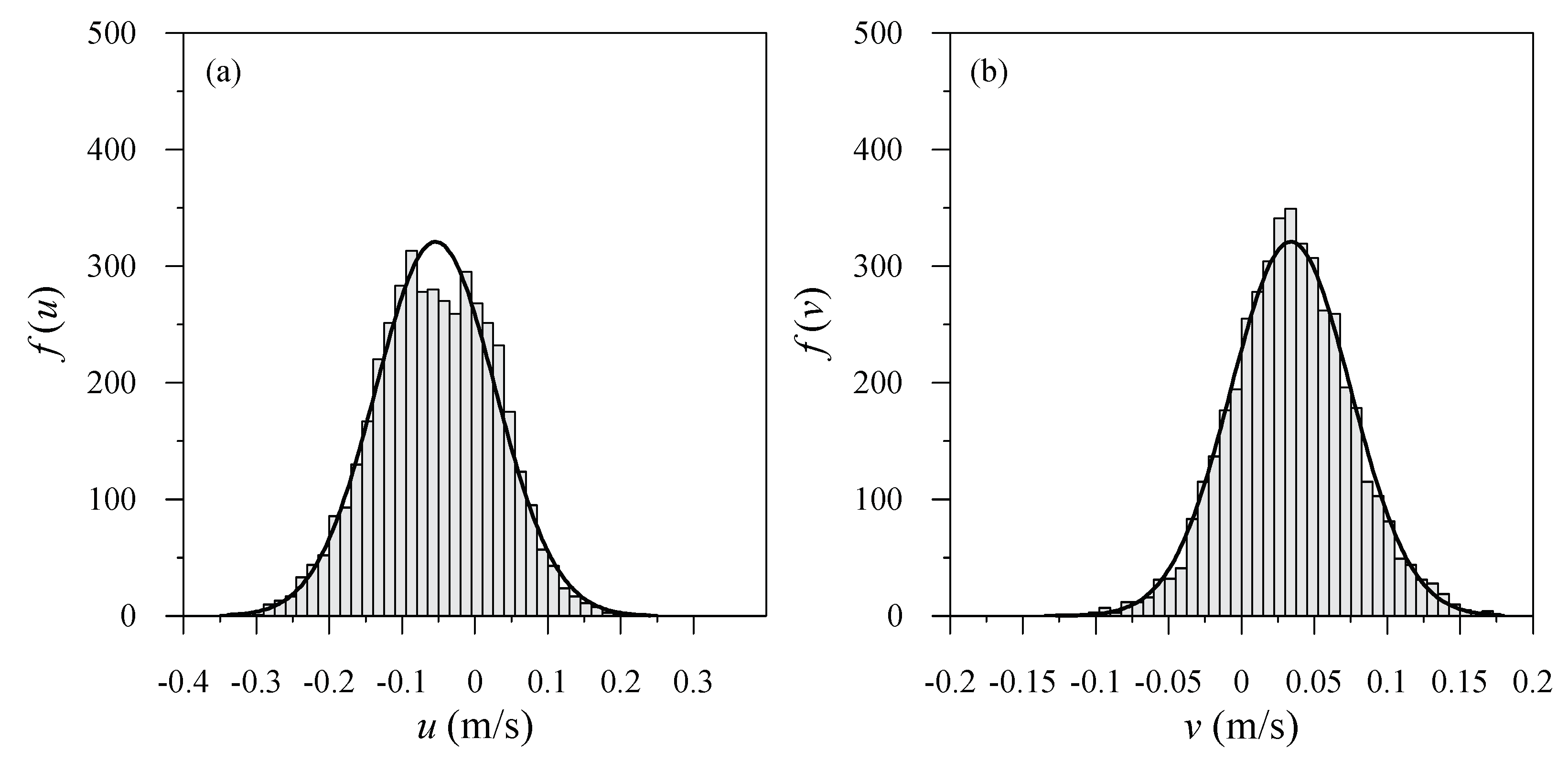
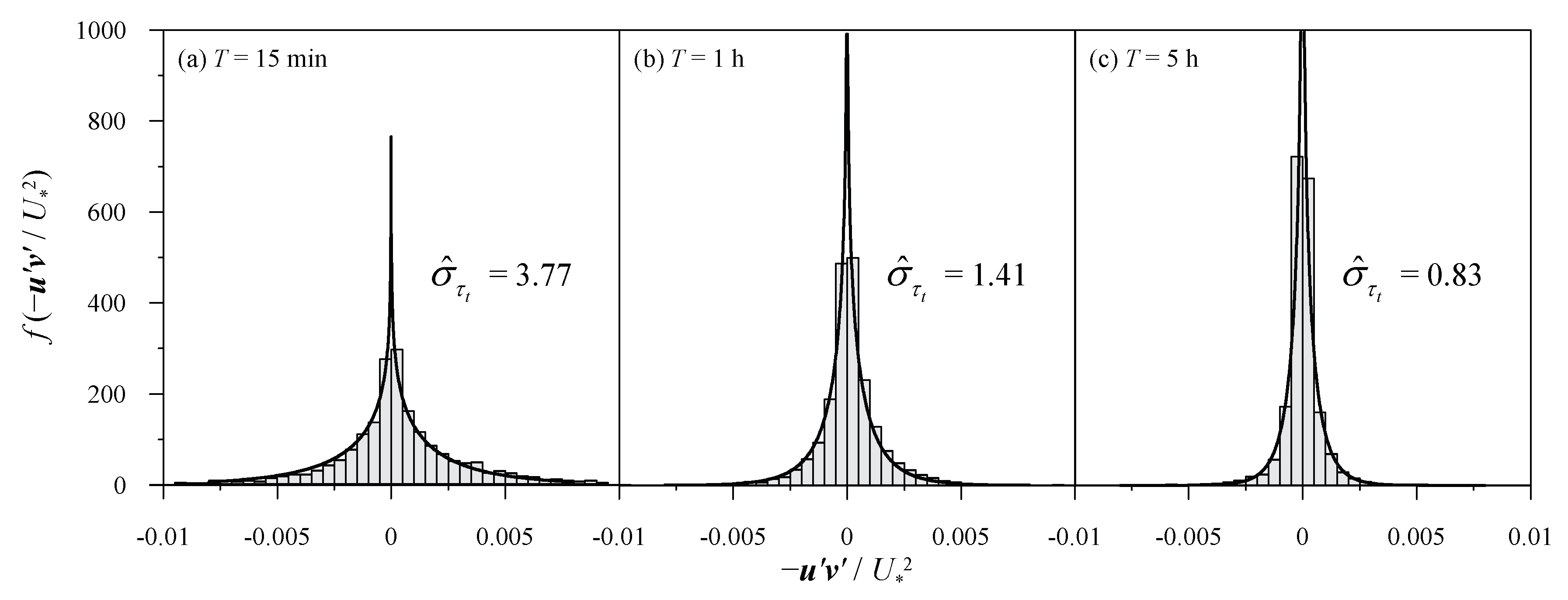
Figure 9 shows the comparisons of the measured longitudinal and vertical flow velocities, and the fitted normal distributions for Run S-2 at $T$ = 15 min. Figure 10 shows the comparisons of the measured probability distributions of $-\mathit{u}\prime \mathit{v}\prime /U_{\ast }{}^2$ and fitted theoretical distributions for Run S-2 at $T$ = 15 min, 1 h, and 5 h. As can be seen in the figure, the theoretical distributions fitted the measured histograms reasonably well. Table 2 reveals that in general ${\hat{\sigma }}_u$ decreases with time for all the experimental conditions, and ${\hat{\sigma }}_v$ decreases with time for Run S-1 and S-2. As a result, the range of the dimensionless Reynolds shear stress $-\mathit{u}\prime \mathit{v}\prime /U_{\ast }{}^2$ also decreases with time in Figure 10, causing a reduction in the extreme values.

Table 3. Summary of the temporal variations in the Reynolds stress and the exceeding probability ($P_{exc}$) at the lowest point of the scour hole.

Run	Time	${\overline{\tau }}_{\mathit{t}}(\mathbf{N}/{\mathbf{cm}}^2)$	${\hat{\sigma }}_{{\tau }_{\mathit{t}}}(\mathbf{N}/{\mathbf{cm}}^2)$	${\mathit{P}}_{\mathit{exc}}$
M-1	15 min	−0.001	1.19	0.133
	1 h	0.042	0.56	0.012
	5 h	0.035	0.53	0.008
M-2	15 min	0.333	1.93	0.136
	1 h	0.061	1.58	0.112
	5 h	−0.013	0.70	0.025
S-1	15 min	0.973	3.56	0.276
	1 h	0.041	0.71	0.027
	5 h	0.066	0.50	0.016
S-2	15 min	0.553	3.77	0.354
	1 h	0.168	1.41	0.135
	5 h	−0.013	0.83	0.039

summarizes the temporal variations in the mean (${\overline{\tau }}_t$) and standard deviation (${\hat{\sigma }}_{{\tau }_t}$) of Reynolds stress and the exceeding probability ($P_{exc}$, defined in Equation (2)) at the lowest point of the scour hole.

Theoretically, the critical shear stress (${\tau }_c$) for a sloping bed needs to be properly adjusted to reflect the gravitational effect (Chiew and Parker [31]). However, in this study we are mainly interested in the ${\tau }_c$ value at the lowest point of the scour hole. It is therefore reasonable to assume that the ${\tau }_c$ value for a plane bed can be adopted. As expected, the ${\hat{\sigma }}_{{\tau }_t}$ value decreases with time for all the experimental conditions. The $P_{exc}$ value also decreases with time as the maximum scour depth gradually approaches the dynamic equilibrium condition.

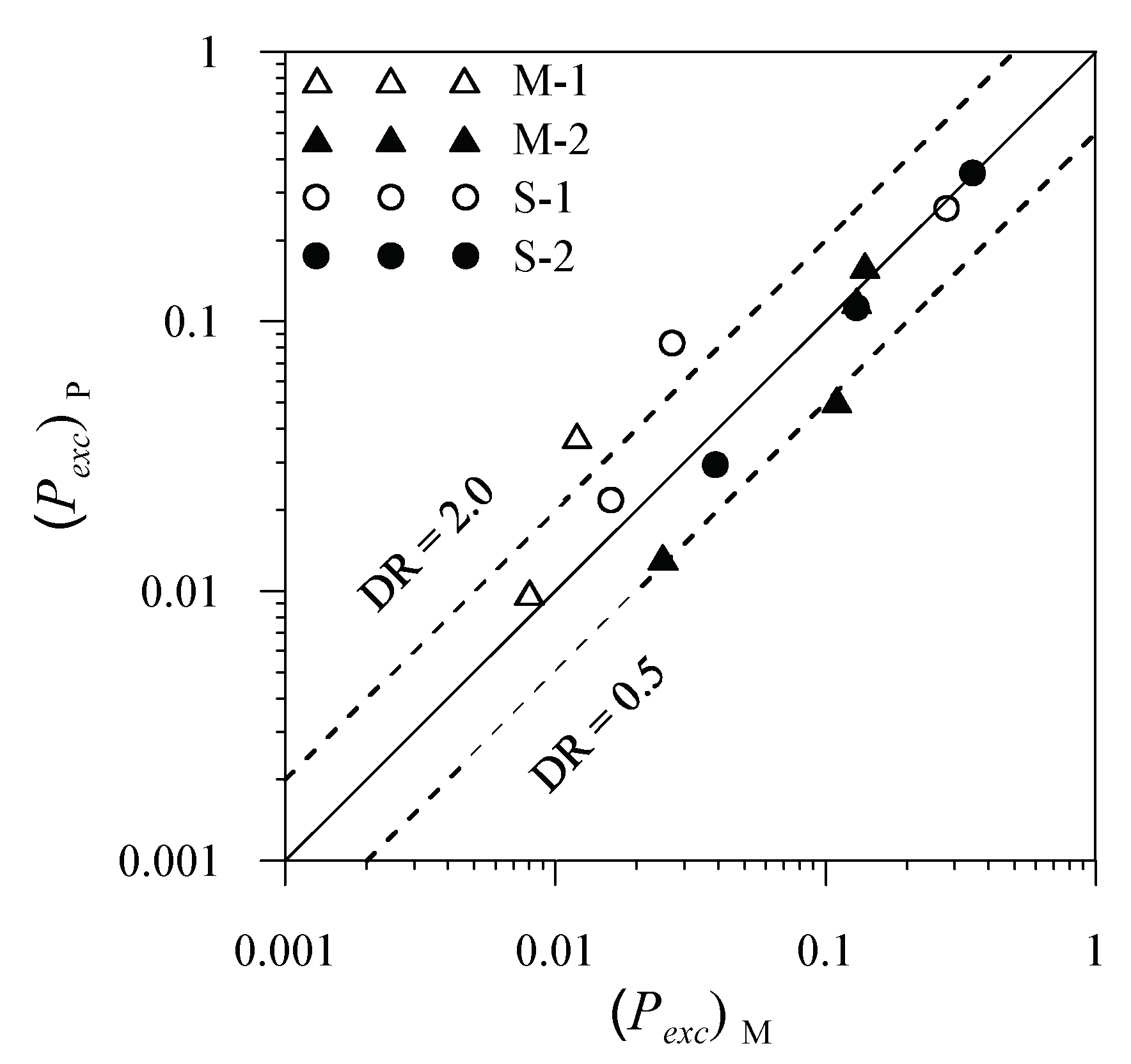
In general, Table 3 reveals that the exceeding probability $P_{exc}$ increases with the flow intensity (bed slope $S_b$ and unit flow discharge $q$). On the basis of the regression analysis, the following equation is developed to provide a qualitative trend of the physical process:

$$P_{exc}=3090\times q^{0.572}\times S_b{}^{1.948}\times T^{-0.831}, r^2=0.94$$

(6)

Figure 11 shows a comparison of the measured and predicted $P_{exc}$ values [${\left(P_{exc}\right)}_{\mathrm{P}}$ vs. ${\left(P_{exc}\right)}_{\mathrm{M}}$], with a determination coefficient $r^2$ = 0.94. Two dashed lines with discrepancy ratios (DR) of 0.5 and 2.0 are plotted in the figure. The discrepancy ratio is defined as the ratio of the predicted $P_{exc}$ value to the corresponding measured value. In general, Equation (6) fitted the data reasonably well. For Run S-1 and Run M-2 at $T$ = 1 h, the deviations are relatively large due to the relatively rugged bed surfaces.

4. Conclusions

Based on the laboratory investigation of the nearly two-dimensional turbulent flows over a movable scour hole downstream of a GCS with a PIV system, the following conclusions can be drawn:

• A PIV system with a high-resolution digital camera, halogen lamps, and ABS seeding particles was adopted and employed to successfully measure the temporal and spatial variations in the flow over the movable scour hole.
• According to the measured vectorial mean velocity profiles (Figure 4), the flow field in the scour hole can be classified into three regions—jet and diffusion, transition, and acceleration regions. Additionally, a recirculation zone was noted near the channel bottom. The reattachment point of the recirculation zone usually moves slowly downstream with time.
• The vertical mean velocity profiles in the diffusion region (between points a and b in Figure 4) of the scour hole can be normalized and fitted with a normal curve (Figure 5, Equation (1)).
• In general, the dimensionless longitudinal turbulence intensity is higher than the dimensionless vertical turbulence intensity, indicating the turbulent flow is anisotropic in the jet and diffusion region. In this study, the distributions of $\mathit{u}\prime /U_{\ast }$ and $\mathit{v}\prime /U_{\ast }$ were similar because there were two local maxima occurring at the entrance and the surface jump. In general, $\mathit{u}\prime /U_{\ast }$ and $\mathit{v}\prime /U_{\ast }$ values decreased with time as the scour hole gradually approached equilibrium.
• By assuming that the longitudinal mean velocity ($u¯$) and vertical mean velocity ($v¯$) are independently and normally distributed, a theoretical Reynolds stress (${\tau }_t=-\rho \mathit{u}\prime \mathit{v}\prime$) distribution can be derived (Equation (5)). The measured Reynolds stress can be fitted with the theoretical equation reasonably well (Figure 10).
• This study demonstrated the significance of the instantaneous shear stress, especially at the early stage of the scouring process, which also quantified Shen and Lu’s [28] findings. Furthermore, the experimental results show that the exceeding probability increased with the unit flow discharge and bed slope, and decreased gradually with time.

References

- Lu, J.Y.; Hong, J.H.; Chang, K.P.; Lu, T.F. Evolution of scouring process downstream of grade-control structures under steady and unsteady flows. Hydrol. Process. 2013, 27, 2699–2709. [Google Scholar] [CrossRef]
- Schoklitsch, A. Kolkbildung unter uberfallstrahlen. Wasserwirtschaft 1932, 24, 341–343. [Google Scholar]
- Bormann, N.E.; Julien, P.Y. Scour downstream of grade-control structures. J. Hydraul. Eng. 1991, 117, 579–594. [Google Scholar] [CrossRef]
- Hoffmans, G.J.C.M.; Verheij, H.J. Scour Manual; Balkema: Rotterdam, The Netherlands, 1997. [Google Scholar]
- Gaudio, R.; Marion, A.; Bovolin, V. Morphological effects of bed sills in degrading rivers. J. Hydraul. Res. 2000, 38, 89–96. [Google Scholar] [CrossRef]
- Gaudio, R.; Marion, A. Time evolution of scouring downstream of bed sills. J. Hydraul. Res. 2003, 41, 271–284. [Google Scholar] [CrossRef]
- Lenzi, M.A.; Marion, A.; Comiti, F.; Gaudio, R. Local scouring in low and high gradient streams at bed sills. J. Hydraul. Res. 2002, 40, 731–739. [Google Scholar] [CrossRef]
- Lenzi, M.A.; Marion, A.; Comiti, F. Local scouring at grade-control structures in alluvial mountain rivers. Water Resour. Res. 2003, 39. [Google Scholar] [CrossRef] [Green Version]
- Lenzi, M.A.; Marion, A.; Comiti, F. Interference processes on scouring at bed sills. Earth Surf. Proc. Land 2003, 28, 99–110. [Google Scholar] [CrossRef]
- Marion, A.; Lenzi, M.A.; Comiti, F. Effect of sill spacing and sediment size grading on scouring at grade-control structures. Earth Surf. Proc. Land 2004, 29, 983–993. [Google Scholar] [CrossRef]
- Marion, A.; Tregnaghi, M.; Tait, S. Sediment supply and local scouring at bed sills in high-gradient streams. Water Resour. Res. 2006, 42. [Google Scholar] [CrossRef] [Green Version]
- Pagliara, S. Influence of sediment gradation on scour downstream of block ramps. J. Hydraul. Eng. 2007, 133, 1241–1248. [Google Scholar] [CrossRef]
- Tregnaghi, M.; Marion, A.; Coleman, S. Scouring at bed sills as a response to flash floods. J. Hydraul. Eng. 2009, 135, 466–475. [Google Scholar] [CrossRef]
- Tregnaghi, M.; Marion, A.; Coleman, S.; Tait, S. Effect of flood recession on scouring at bed sills. J. Hydraul. Eng. 2010, 136, 204–213. [Google Scholar] [CrossRef]
- Wu, S.; Rajaratnam, N. Submerged flow regimes of rectangular sharp-crested weirs. J. Hydraul. Eng. 1996, 122, 412–414. [Google Scholar] [CrossRef]
- Guan, D.W.; Melville, B.W.; Friedrich, H. Live-bed scour at submerged weirs. J. Hydraul. Eng. 2015, 141. [Google Scholar] [CrossRef]
- Guan, D.W.; Melville, B.; Friedrich, H. Local scour at submerged weirs in sand-bed channels. J. Hydraul. Res. 2016, 54, 172–184. [Google Scholar] [CrossRef]
- Guan, D.W.; Melville, B.W.; Friedrich, H. Flow patterns and turbulence structures in a scour hole downstream of a submerged weir. J. Hydraul. Eng. 2014, 140, 68–76. [Google Scholar] [CrossRef]
- Gaudio, R.; Tafarojnoruz, A.; Calomino, F. Combined flow-altering countermeasures against bridge pier scour. J. Hydraul. Res. 2012, 50, 35–43. [Google Scholar] [CrossRef]
- Ferraro, D.; Tafarojnoruz, A.; Gaudio, R.; Cardoso, A.H. Effects of pile cap thickness on the maximum scour depth at a complex pier. J. Hydraul. Eng. 2013, 139, 482–491. [Google Scholar] [CrossRef]
- Powell, D.M. Flow resistance in gravel-bed rivers: Progress in research. Earth-Sci. Rev. 2014, 136, 301–338. [Google Scholar] [CrossRef]
- Bathurst, J.C.; Li, R.M.; Simons, D.B. Resistance equation for large-scale roughness. J. Hydraul. Div. 1981, 107, 1593–1613. [Google Scholar]
- Lawrence, D.S.L. Macroscale surface roughness and frictional resistance in overland flow. Earth Surf. Proc. Land 1997, 22, 365–382. [Google Scholar] [CrossRef]
- Nezu, I.; Rodi, W. Open-channel flow measurements with a laser doppler anemometer. J. Hydraul. Eng. 1986, 112, 335–355. [Google Scholar] [CrossRef]
- Lu, J.Y.; Chen, J.Y.; Chang, F.H.; Lu, T.F. Characteristics of shallow rain-impacted flow over smooth bed. J. Hydraul. Eng. 1998, 124, 1242–1252. [Google Scholar] [CrossRef]
- Dodaro, G.; Tafarojnoruz, A.; Stefanucci, F.; Adduce, C.; Calomino, F.; Gaudio, R.; Sciortino, G. An experimental and numerical study on the spatial and temporal evolution of a scour hole downstream of a rigid bed. In Proceedings of the International Conference on Fluvial Hydraulics, River Flow, Lausanne, Switzerland, 3–5 September 2014; pp. 1415–1422. [Google Scholar]
- Dodaro, G.; Tafarojnoruz, A.; Sciortino, G.; Adduce, C.; Calomino, F.; Gaudio, R. Modified Einstein sediment transport method to simulate the local scour evolution downstream of a rigid bed. J. Hydraul. Eng. 2016, 142. [Google Scholar] [CrossRef]
- Shen, H.W.; Lu, J.Y. Development and prediction of bed armoring. J. Hydraul. Eng. 1983, 109, 611–629. [Google Scholar] [CrossRef]
- Kim, H.Y. Statistical notes for clinical researchers: Assessing normal distribution (2) using skewness and kurtosis. Restor. Dent. Endod. 2013, 38, 52–54. [Google Scholar] [CrossRef] [PubMed]
- Lu, J.Y.; Lee, J.J.; Lu, T.F.; Hong, J.H. Experimental study of extreme shear stress for shallow flow under simulated rainfall. Hydrol. Process. 2009, 23, 1660–1667. [Google Scholar] [CrossRef]
- Chiew, Y.-M.; Parker, G. Incipient sediment motion on non-horizontal slopes. J. Hydraul. Res. 1994, 32, 649–660. [Google Scholar] [CrossRef]
Figure 1.
Plane view of the experimental channel (not to scale).
Figure 2.
Maximum scour depth evolution for Run S-2.
Figure 3.
Comparison of the measured dimensionless longitudinal turbulence intensity profiles in the fully developed zone with the empirical profiles presented by Nezu and Rodi [24] at: (a) = 8.41 m, (b) = 8.48 m, and (c) = 8.55 m.
Figure 4.
Measured vectorial mean velocity profiles in the scour hole for Run S-2: (a) = 15 min, (b) = 1 h, and (c) = 5 h.
Figure 5.
Comparison of the normalized mean velocity profiles in zone ab (Figure 4).
Figure 6.
Measured dimensionless longitudinal turbulence intensity () contours in the scour hole for Run S-2: (a) = 15 min, (b) = 1 h, and (c) = 5 h.
Figure 7.
Measured dimensionless vertical turbulence intensity () contours in the scour hole for Run S-2: (a) = 15 min, (b) = 1 h, and (c) = 5 h.
Figure 8.
Variations in the dimensionless Reynolds shear stress () and the exceeding probability () along the boundary of the scour hole at (a) = 15 min, (b) = 1 h, and (c) = 5 h.
Figure 9.
Comparisons of the measured flow velocities and fitted normal distributions for Run S-2 ( = 15 min): (a) and (b) .
Figure 10.
Comparisons of the measured probability distributions of and fitted theoretical distributions (Equation (5)) for Run S-2: (a) = 15 min, (b) = 1 h, and (c) = 5 h.
Figure 11.
Comparison of the measured and predicted exceeding probabilities (DR = Predicted /Measured ).